以雙鏡面環場攝影機及自動車作人行道上導盲犬之研究

國

立

交

通

大

學

多媒體工程研究所

碩 士 論 文

以雙鏡面環場攝影機及自動車作人行道上導盲

犬之研究

A Study on Construction of a Machine Guide Dog

Using a Two-mirror Omni-camera and an

Autonomous Vehicle on Sidewalks

研 究 生：黃致瑋

以雙鏡面環場攝影機及自動車作人行道上導盲犬之研究

A Study on Construction of a Machine Guide Dog Using a

Two-mirror Omni-camera and an Autonomous Vehicle on

Sidewalks

研 究 生：黃致瑋 Student：Chih-Wei Huang

指導教授：蔡文祥 Advisor：Wen-Hsiang Tsai

國 立 交 通 大 學

多 媒 體 工 程 研 究 所

碩 士 論 文

Submitted to Institute of Computer Science and Engineering College of Computer Science

National Chiao Tung University in partial Fulfillment of the Requirements

for the Degree of Master

in

Computer Science

June 2012

Hsinchu, Taiwan, Republic of China

A Study on Construction of a Machine Guide Dog

Using a Two-mirror Omni-camera and an

Autonomous Vehicle on Sidewalks

Student: Chih-Wei Huang

Advisor: Wen-Hsiang Tsai

Institute of Multimedia Engineering

College of Computer Science

National Chiao Tung University

ABSTRACT

Various techniques for construction of a machine guide dog using a two-mirror omni-camera and an autonomous vehicle for navigations on sidewalks are proposed. The autonomous vehicle can compute 3D information from acquired omni-images to localize itself using pre-selected landmarks, and guide a blind person to follow a planned path to a destination on a sidewalk. Firstly, a method for learning the sidewalk environment is proposed to construct a navigation map, including a navigation path, along-path landmark locations, and relevant vehicle guidance parameters. Next, a navigation system with self-localization and automatic guidance capabilities using landmarks including curb lines, tree trunks, stop lines on roads, lawn corners, traffic cones, and signboards is proposed. By the use of a space-mapping technique, three space line detection techniques for use directly on the omni-image are proposed, which can be used to compute the 3D position of a specific space line in the shape of a sidewalk landmark.

are proposed. Using these vehicle self-localization techniques, imprecise vehicle positions due to incremental mechanic errors can be adjusted. In addition, for the purpose of continuous navigation, a curb line following technique is proposed as well to guide the vehicle along a sidewalk when landmarks are not available during the navigation process. To detect landmarks in the outdoor environment, techniques for dynamic threshold adjustments are also proposed for adapting the system’s capability to varying lighting conditions in navigation environments.

Good experimental results showing the flexibility and feasibility of the proposed methods for real applications are also included.

以雙鏡面環場攝影機及自動車作人行道上導盲犬之研

究

研究生：黃致瑋

指導教授：蔡文祥 博士

國立交通大學多媒體工程研究所

摘要

ACKNOWLEDGEMENTS

The author is in hearty appreciation of the continuous guidance, discussions, and support from his advisor, Dr. Wen-Hsiang Tsai, not only in the development of this thesis, but also in every aspect of his personal growth.

Appreciation is also given to the colleagues of the Computer Vision Laboratory in the Institute of Computer Science and Engineering at National Chiao Tung University for their suggestions and help during his thesis study.

Finally, the author also extends his profound thanks to his dear mom and dad for their lasting love, care, and encouragement.

CONTENTS

ABSTRACT (in English)……….….i

ABSTRACT (in Chinese)………iii

ACKNOWLEDGEMENTS………iv

CONTENTS………..v

LIST OF FIGURES………....vii

LIST OF TABLES………...xi

1.2 Survey of Related Works ... 3

1.3 Overview of Proposed System ... 5

1.4 Contribution of This Study ... 8

1.5 Thesis Organization ... 9

Chapter 2 System Design and Processes ... 10

2.1 Ideas of System Design ... 10

2.2 System Configuration ... 11

2.2.1 Hardware configuration ... 11

2.2.2 Structure of used two-mirror omni-camera ... 15

2.2.3 Software configuration ... 18

2.3 3D Data Acquisition by the Two-mirror Omni-camera ... 19

2.3.1 Review of imaging principle of two-mirror omni-camera ... 19

2.3.2 Derivation of formulas for 3D data acquisition ... 20

2.4 System Operation Processes ... 24

2.4.1 Learning process ... 24

2.4.2 Navigation process ... 25

Chapter 3 Learning Strategy for Automatic Navigation ... 28

3.1 Introduction ... 28

3.1.1 Selected landmarks in outdoor environments for this study ... 28

3.1.2 Camera calibration ... 29

3.1.3 Learning of guidance parameters ... 29

3.2 Camera Calibration by Space-mapping Approach ... 31

3.3 Coordinate Systems ... 34

3.5 Learning Processes for Creating a Navigation Path ... 41

3.5.1 Strategy for learning landmark positions and related vehicle poses ... 42

3.5.2 Learning of fixed obstacles in a navigation path ... 44

3.5.3 Algorithm for path learning ... 45

Chapter 4 Navigation Strategy in Outdoor Environments... 50

4.1 Strategy for Automatic Navigation ... 50

4.1.1 Vehicle localization by alone-path objects ... 50

4.1.2 Dynamic Adjustment learning parameters in navigation process 50 4.2 Guidance Technique in Navigation Process ... 51

4.2.1 Principle of proposed navigation process ... 51

4.2.2 Automatic vehicle localization by selected landmarks on sidewalks ... 53

4.2.3 Fixed-obstacle avoidance process ... 58

4.3 Detailed Algorithm of Navigation Process ... 59

Chapter 5 Natural Landmarks Detection in Images Using New Space Line Detection Technique ... 64

5.1 Idea of Proposed Space Line Detection Technique ... 64

5.2 Proposed Technique for Space Line Detection ... 65

5.2.1 Line detection using pano-mapping table ... 66

5.2.2 3D data computation using three space lines ... 73

5.3 Proposed Method for Tree Trunk Detection... 78

5.3.1 Tree trunk contour description ... 78

5.3.2 Moment-preserving thresholding for tree trunk segmentation... 81

5.3.3 Tree trunk localization ... 82

5.3.4 Experimental results for tree trunk detection ... 83

5.4 Proposed Method for Lawn Corner Detection ... 85

5.4.1 Lawn corner detection and localization ... 86

5.4.2 Experimental results for lawn corner detection ... 88

Chapter 6 Artificial Landmarks Detection in Images Using Space Line Detection Technique ... 90

6.1 Proposed Technique for Curb Line Following ... 90

6.1.1 Review of adopted curb line following ... 90

6.1.2 Proposed curb line localization technique... 93

6.1.3 Experimental results of curb line detection ... 94

6.2 Proposed Method for Signboard Detection ... 96

6.2.2 Signboard position computation ... 99

6.2.3 Experimental results of signboard detection ... 101

6.3 Proposed Method for Detecting Stop Lines on Roads ... 102

6.3.1 Detection and localization of stop lines on roads ... 103

6.3.2 Experimental results of detection of stop lines on roads... 106

6.4 Proposed Method for Detecting and Localizing Traffic cones ... 108

6.4.1 Detection and localization of traffic cones ... 108

6.4.2 Experimental results of traffic cone detection ... 110

Chapter 7 Experimental Results and Discussions ... 113

7.1 Experimental Results ... 113

7.2 Discussions ... 118

Chapter 8 Conclusions and Suggestions for Future Works ... 120

8.1 Conclusions ... 120

8.2 Suggestions for Future Works ... 121

LIST OF FIGURES

Figure 1.1 Flowchart of proposed learning stage. ... 7 Figure 1.2 Flowchart of navigation stage. ... 8 Figure 2.1 Three different views of the used hardware architecture, which includes a vehicle and a stereo camera. (a) A 45o view. (b) A front view. (c) A side view. ... 12 Figure 2.2 The Autonomous vehicle, Pioneer 3-DX, produced by MobileRobots Inc., used in this study. (a) A back view. (b) A front view. ... 13 Figure 2.3 The camera system used in this study. ... 14 Figure 2.4 The used camera and lens. (a) The camera of model Arcam-200so produced by ARTRAY Co. (b) The lens produced by Sakai Co. ... 14 Figure 2.5 The laptop computer of model TOSHIBA R840 used in this study. ... 15 Figure 2.6 An illustration of the two-mirror omni-camera and a space point projected on the CMOS sensor of the camera. ... 17 Figure 2.7 The reflection property of the two hyperboloidal-shaped mirrors in the camera system. ... 17 Figure 2.8 Two different placements of the two-mirror omni-camera on the vehicle and the region of overlapping. (a) The optical axis going through the two mirrors is parallel to the ground. (b) The optical axis through the two . ... 18 Figure 2.9 Imaging principle of a space point G using an omni-camera. ... 20 Figure 2.10 The cameras coordinate systemCCSlocal, and a space point G projected on

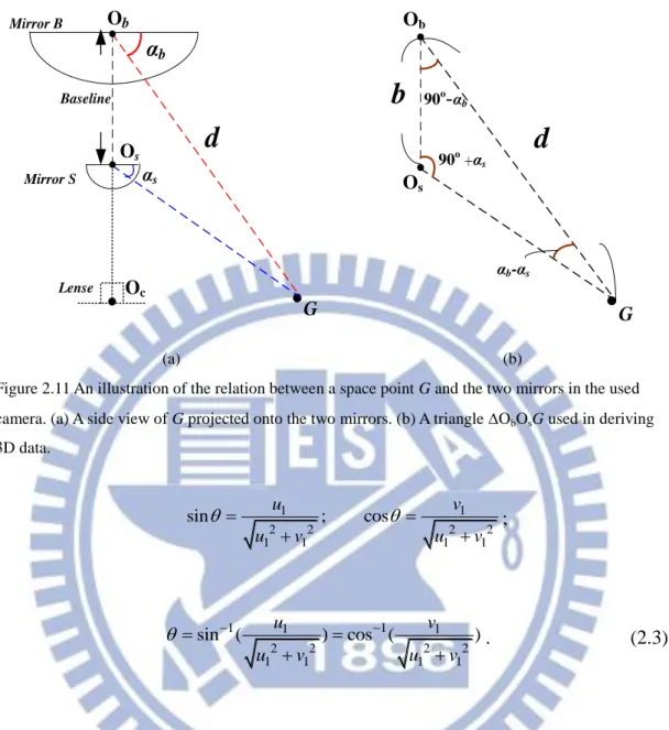
the omni-image acquired by the two-mirror omni-camera. ... 21 Figure 2.11 An illustration of the relation between a space point G and the two mirrors in the used camera. (a) A side view of G projected onto the two mirrors. (b) A triangle ObOsG used in deriving 3D data. ... 22

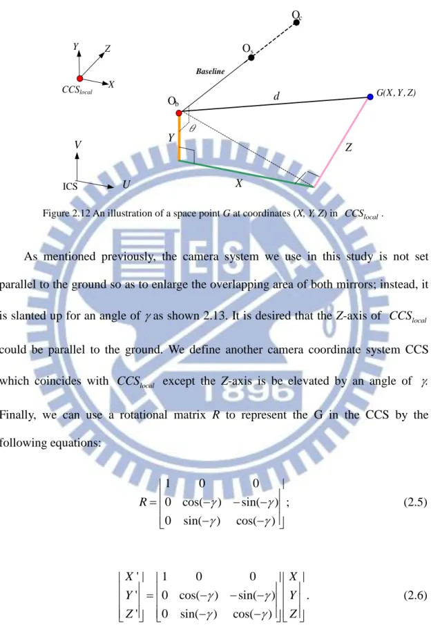
Figure 2.12 An illustration of a space point G at coordinates (X, Y, Z) in CCSlocal. . 23

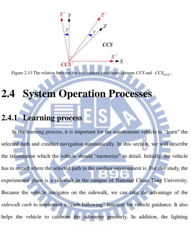
Figure 2.13 The relation between the two camera coordinate systems CCS and

local

CCS . ... 24 Figure 2.14 Learning process. ... 26 Figure 2.15 Navigation process... 27 Figure 3.1 Two types of natural landmarks selected for use in this study. (a) Tree landmark. (b) Lawn corner point. ... 29 Figure 3.2 Three artificial landmarks used in this study. (a) Tree landmark. (b) Road stop line landmark. (c) Signboard landmark... 30 Figure 3.3 Illustration of constructing pano-mapping tables in this study. ... 33 Figure 3.4 Four coordinate systems used in this study. (a) The ICS. (b) The CCS. (c)

The VCS. (d) The GCS. ... 35 Figure 3.5 A vehicle at coordinates (Cx, Cy) with a rotation angle θ with respect to

the GCS. ... 36 Figure 3.6 An illustration of the relation between the CCS and the VCS. ... 36 Figure 3.7 A pair of environment windows for road stop line detection. ... 37 Figure 3.8 Two different illuminations for curb line detection. (a) An instance of overexposure. (b) A suitable case. ... 39 Figure 3.9 Two different illuminations for signboard detection. (a) An instance of underexposure. (b) A suitable case. ... 40 Figure 3.10 The process for learning landmark segmentation parameters. ... 41 Figure 3.11 A fixed obstacle in a navigation path which may cause the vehicle to fall outside the sidewalk. ... 42 Figure 3.12 A learning interface for the trainer to learn the position of the fixed obstacle by clicking mouse on corresponding points in the image region of Mirror B. ... 46 Figure 3.13 The process for navigation path creation. ... 49 Figure 4.1 Two conditions to decide if the vehicle arrives at the next node in the navigation process. (a) According to the distance between the vehicle position and the next node position. (b) According to the distance between the next node position and the position of the projection of the vehicle on the vector connecting the current node and the next node. ... 53 Figure 4.2 Proposed node-based navigation process. ... 54 Figure 4.3 Proposed odometer reading adjustment process. ... 57 Figure 4.4 A recorded vehicle position V and the current vehicle position V in the GCS. ... 58 Figure 4.5 Landmark detection for vehicle localization at position T. (a) At coordinates (lx, ly) in VCS. (b) At coordinates (Cx, Cy) in GCS. ... 58

Figure 4.6 Process of odometer calibration position is far off the curb line. The vehicle detects the curb line at V1 to calibrate the orientation and then

navigates to V2 to calibrate the position using landmark. ... 60

Figure 4.7 Process of fixed obstacle avoidance. We insert the Nodeavoid1, Nodeavoid2,

and Nodeavoid3.for obstacle avoidance in the original navigation path. .. 61

Figure 4.8 Flowchart of detailed proposed navigation process... 63 Figure 5.1 Wu and Tsai [25] proposed a line detection method for the omni-image to conduct automatic helicopter landing. (a) Illustration of automatic helicopter landing on a helipad with a circled H shape. (b) An omni-image of a simulated helipad... 65

Figure 5.3 A space line L projected on IL in an omni-image. ... 68

Figure 5.4 Three specific space lines. ... 72 Figure 5.5 A space line projected onto IL1 and IL2 on two mirrors in the used

two-mirror omni-camera. ... 74 Figure 5.6 A space line projected onto IL3 and IL4 on two mirrors in the used

two-mirror omni-camera. ... 76 Figure 5.7 A space line projected onto IL5 and IL6 on two mirrors in the used

two-mirror omni-camera. ... 77 Figure 5.8 Proposed method for tree trunk localization. ... 78 Figure 5.9 Principal component analysis for the tree trunk contour. (a) Illustrated principal components, e1 and e2, on the omni-image. (b) A rotation angle

 between the ICS and the computed principal components. ... 80 Figure 5.10 The input image with a tree trunk. ... 84 Figure 5.11 Tree trunk segmentation by moment-preserving thresholding. ... 84 Figure 5.12 The result of tree truck detection and its position. (a) The result image of extracting the vertical axis line of the tree trunk. (b) The related tree truck position with respect to the vehicle position. ... 85 Figure 5.13 Two different camera systems take the lawn corner. (a) By digital camera. (b) By omni-camera. ... 86 Figure 5.14 Two different directions in the image for lawn corner detection. ... 89 Figure 5.15 Two result of LX line detection. ... 89

Figure 6.1 A detected curb line and the inner boundary points of the curb line on the omni-image. ... 91 Figure 6.2 Two images of curb segmentation resulting from using different threshold values (a) The segmentation result with original threshold value. (b) The segmentation result image by dynamic thresholding. ... 92 Figure 6.3 An omni-image with curb line landmark. ... 95 Figure 6.4 The curb line detection method proposed by Chou and Tsai (a) the curb line segmentation result. (b) Illustration of extracted curb boundary points and a fitting line. ... 95 Figure 6.5 The curb line detection method (a) the curb line segmentation result. (b) The related curb line position with respect to the vehicle position. ... 95 Figure 6.6 Proposed method of signboard localization. ... 97 Figure 6.7 The omni-image with a signboard. ... 101 Figure 6.8 Two result images of signboard segmentation with different threshold values (a) The result of signboard segmentation with original threshold value. (b) The result image of signboard segmentation by dynamic thresholding. ... 102

Figure 6.9 The result of signboard detection and obtained signboard position. (a) The result image of extracting the LY line of the signboard (b) The

related signboard position with respect to the vehicle position. ... 102 Figure 6.10 Two obtained corners of Cin and Cout of a stop line on the road in the

CCS. ... 106 Figure 6.11 The omni-image with a stop line on the road. ... 107 Figure 6.12 The result of stop line segmentation by the Canny edge detector. ... 107 Figure 6.13 The result of stop line on detection and position computation. (a) The resulting image of extracting the LX and LZ lines of the stop line. (b) The

relative position of the stop line with respect to the vehicle position. .. 108 Figure 6.14 The omni-image with a traffic cone. ... 111 Figure 6.15 The result of traffic cone segmentation using the Canny edge detector. .... ... 111 Figure 6.16 The result of traffic cone detection and the obtained position of the traffic cone. (a) The result image of extracting the LX, LY, and LZ lines of

the traffic cone (b) The relative position of the traffic cone with respect to the vehicle position. ... 112 Figure 7.1 The experimental environment. (a) A side view. (b) Illustration of the environment. ... 113 Figure 7.2 The Learning interface of the proposed vehicle system. ... 114 Figure 7.3 Learning of a fixed obstacle. (a) The position of fixed obstacle on the omni-image (Lime-colored points clicked by the trainer). (b) Computed fixed obstacle positions in the real world. ... 115 Figure 7.4 Illustration of the learned navigation path. ... 116 Figure 7.5 Some results of landmark detection. (a) A tree trunk detection result with LY line drawn in red. (b) A traffic cone detection result with LX, LY, and

LZ line drawn in dark blue, lime, and navy blue, respectively. (c) A lawn

corner detection result with two boundary lines drawn in navy blue. (d) The result of stop line with three boundary lines drawn in yellow and navy blue, respectively. (e) A signboard detection result with LY line

drawn in red and lime, respectively. ... 116 Figure 7.6 The result of curb line detection. ... 117 Figure 7.7 The vehicle reads the fixed obstacle position from the navigation path and change the path to avoid it. (a)~(d) show the process of fixed obstacle avoidance. ... 117 Figure 7.8 The recorded path map in the navigation process. (Blue points represent the vehicle path and other points with different color represent different

LIST OF TABLES

Table 2.1 The specification of Arcam-200so. ... 14 Table 2.2 Specification of the laptop computer. ... 16 Table 2.3 Specifications of the used two hyperboloidal-shaped mirrors. ... 16 Table 3.1 Two pano-mapping tables used for the two-mirror omni-camera used in this study. (a) Pano-mapping table used for Mirror B. (b) Pano-mapping table used for Mirror S. ... 34 Table 3.2 Eleven different types of navigation path nodes. ... 48 Table 6.1 Comparison of two methods for curb line detection. ... 96 Table 7.1 Precision of estimated landmark positions and their error percentages.

119

Chapter 1

Introduction

1.1 Motivation

There are millions of blind people in the world. Some of them use blind canes to travel on the road. However, blind canes can only be used to detect obstacles at short distances by blind people. Besides using blind canes, a better choice is to use guide dogs. Guide dogs can assist blind people to avoid obstacles and walk in indoor or outdoor environments smoothly even if there is no barrier-free facility along the way. For the welfare of blind people, guide dogs not only improve the safety, but also enhance the quality, of their lives.

However, there are few guide dogs in Taiwan. According to the information provided by Taiwan Guide Dog Association [20] and Taiwan Foundation for the blind [21] in 2012, there are almost sixty thousand blind people but just twenty-eight guide dogs in Taiwan. This rate is too low to provide sufficient supports for the blind people. The reasons why guide dogs are so few are listed below:

1. only certain breeds of dogs can be trained as guide dogs;

2. a trainer has to spend very much time to teach a young guide dog;

3. the individual difference between the personalities of the master and the guide dog is a problem which should be solved;

4. it costs at least one million NT dollars to train a guide dog.

It is wished in this study to utilize technology and knowledge to solve this problem of guide dog shortage, so we follow the idea of providing a machine guide dog for each blind person. Each machine guide dog can be a replacement for a real

machine guide dog basically is constructed by the use of an autonomous vehicle and a camera. To implement a machine guide dog, it is desired that a vision-based autonomous vehicle can automatically navigate in outdoor environments and keep watch over the camera’s field of view (FOV) automatically. It is also hoped that when the vehicle detects a risk area like a hole or an obstacle along the way, it can safely guide the blind person to avoid the danger; and when the autonomous vehicle reaches the destination, it will inform the blind person so.

For this purpose, the critical problem is how to navigate a vision-based autonomous vehicle successfully in outdoor environments. Normally, an autonomous vehicle is equipped with an odometer, and we can use the odometer readings to compute the current position of the vehicle with respect to its initial position of a navigation session. However, the position which the odometer provides is often not sufficiently precise because the autonomous vehicle usually suffers from incremental mechanic errors due to manufacturing imprecision. One good solution is to continually estimate the vehicle position by monitoring natural or artificial objects in the surroundings along the navigation path, which is a sidewalk in this study.

In normal cases, a blind person has to pass regular scenes with objects along sidewalks, so we may train the autonomous vehicle beforehand to recognize the path and the surrounding objects, just like training a guide dog in the place. That is to say, we may let the autonomous vehicle to “remember” along-path landmarks in advance, and construct the on-board navigation system to capture the current landmark information during each navigation session.

In summary, the goal of this study is to develop a vision-based autonomous vehicle for use as a machine guide dog on sidewalks. The system is expected to possess the following capabilities:

2. learning common landmarks along sidewalks;

3. navigating automatically along sidewalks using learned landmarks for localization;

4. navigating to goals successfully on learned paths.

1.2 Survey of Related Works

In this section, we conduct a survey of related works about assistances to the blind people, including new application systems for the blind, localization techniques in indoor or outdoor environments, and landmark detection via the use of stereo omni-cameras.

More and more research results about developing walking aids for the blind people have appeared. As an improvement on the blind cane, an easy way is to install a sensor device on a blind cane so as to detect obstacles at a certain distance. Borenstein and Ulrich [1] developed the “GuideCane” which can detect obstacles by ultrasonic sensors to help blind people to pass dangerous areas. Some helpful navigation systems for the blind were also proposed. Ivanchenko et al. [2] proposed a system for impaired wheelchair users to detect the presence of obstacles or other terrain features by computer vision techniques and warn the user. A robotic travel aid (RTA) called HITOMI was proposed by Mori et al. [3] which can detect vehicles and pedestrians using multiple sensors. Besides, Hsieh [4] utilized two cameras installed on a cap to find accessible obstacles and regions in unknown environments and alert the impaired person by voice. Likewise, Shang [5] used two cameras assembled on the shoulder to walk independently in known or unknown environments.

and rooms. Lisa et al. [7] utilized a DGPS (differential GPS) device to localize a blind person in indoor and outdoor environments. Also, Chen and Tsai [8] proposed an indoor autonomous vehicle navigation system using ultrasonic sensors. In outdoors, the GPS can be used as a localization system for the vehicle [9].

Furthermore, vision-based sensors have been widely utilized for vehicle navigation. Atiya and D. Hager [10] proposed the vision-based system which computes the location in real-time. Chen and Tsai [11] proposed a vehicle localization technique which modifies the position of a vehicle by keeping watch over learned objects. Another method of vehicle localization in indoor environments by watching house corners was proposed by Chiang and Tsai [12]. Moreover, a system which uses stereo cameras and a low-cost GPS sensor was proposed by Agrawal and Konolige [13]. Tsai and Tsai [14] used a PTZ camera and an ultrasonic sensor to direct vehicle patrolling and people following successfully. Another application using a combination of cameras and other devices was proposed by Lopez et al. [15], who connected a laser and a robot’s camera to compute the robot location.

An omni-directional camera has the advantage of having a large FOV in contrast with a traditional CCD camera. Because of this advantage, we choose to use the omni-camera to design the machine guide dog system in this study. So, we conduct a survey of related works about vehicle navigation systems using omni-cameras as well here. To enhance the accuracy of localization, Lui and Jarvis [16] implemented an algorithm which implements omni-directional vision on a GPU. To detect landmarks in environments, Fu et al. [17] proposed a navigation system with embedded omni-vision for landmark recognition. A method which was conducted to achieve vehicle self-localization by matching omni-directional images was proposed by Ishizuka et al [18]. Wu and Tsai [19] detected circular landmarks on ceilings to

1.3 Overview of Proposed System

The goal of this study is to lead a vision-based machine guide dog to navigate in outdoor environments automatically. The most important task to achieve this goal is vehicle localization. The method for vehicle localization we propose is to detect

landmarks along the path. Besides, some strategies for navigation on the learned path are proposed for use in this system. In this section, we will introduce the vision-based autonomous vehicle system which we use in this study. The operation process of this system may be divided into two stages: the learning stage and the navigation stage. The learning stage includes primarily the task of training the autonomous vehicle to acquire the along-path information useful for vehicle guidance before navigation. Then, we conduct vehicle navigation along the path which we pre-select in the navigation stage. The details of the two stages are illustrated in Figs. 1.1 and 1.2, respectively, and discussed in the following.

A. The learning stage

In the process of learning which is necessary before the vehicle can navigate, at first we combine the camera system into the autonomous vehicle. Unfortunately, the camera system does not perfectly match the vehicle’s structure. It should so be calibrated to find the relation between the image coordinates and the real-world locations. In this system, we utilize a two-mirror omni-camera system as the visual sensor. Because of the special structure of the two-mirror omni-camera system, its parameters cannot be acquired and calculated easily. Therefore, we adopt a space-mapping method proposed by Jeng and Tsai [20] to solve the problem. We get accordingly a space-mapping table, called pano-table, to calibrate the camera system instead. After we finish the calibration work, we can obtain the range data of

the navigation. Secondly, we learn relevant path information for vehicle guidance, including the environment parameters, the vehicle position in the path, the location of each used landmark, and some landmark segmentation parameters.

After we guide the vehicle to a particular spot, a path learning work is started. In this phase of the learning stage, we propose the use of two navigation modes: one being navigation by following the sidewalk; the other manual control by the trainer. If we choose the first mode, the autonomous vehicle starts to navigate to the goal and the information of the vehicle pose at each visited spot is recorded. If we want the system to “memorize” a specific landmark along the path, we can use the second mode to achieve the landmark information acquisition and position estimation. Besides, each path we choose is along a sidewalk in an outdoor environment, and some information about the outdoor environment along the path is also recorded during this phase of learning. Finally, all of the data so learned are integrated into a set of path information.

B. The navigation stage

As we mentioned above, the path information which is acquired in the learning stage is used in the navigation stage. In the navigation stage, three major works are conducted by the vehicle. One is moving forward, another is obstacle detection, and the third is vehicle location estimation and modification.

Generally, the vehicle can move forward continually toward the goal we pre-select. Between every two nodes in a path, the vehicle can choose one of two navigation modes─ navigation by the vehicle odometer (called the blind navigation mode) and navigation by the side walk. When the navigation by the side walk mode is

selected, the vehicle detects the sidewalk curb with a prominent color continually and adopts a line following technique to guide the vehicle. When no curb can be used

odometer mode and moves forward “blindly” according to the odometer reading on

the pre-selected path. Also, it is desired to find fixed obstacles and have a strategy to pass dangerous areas.

Calibration the camera system on vehicle Begin to learn a navigation path Environment information Navigation by Sidewalk following Manual navigation by user Landmark detection Landmark localization Vehicle pose information Landmark position information The navigation path information End learning

Path information Start navigation Sidewalks navigation Blind navigation Obstacle detection Obstacle avoidance Landmark detection and localization Vehicle position modification End navigation

Figure 1.2 Flowchart of navigation stage.

Moreover, we use some objects which are commonly seen along sidewalks, such as trees, road stop lines, traffic cones, signboards, and corner points of the lawn, to localize the vehicle in this study. That is, we modify the vehicle position with respect to each located landmark to eliminate accumulated mechanical or vision-processing errors during the navigation process. Finally, we propose three new vertical space line detection methods to calculate the locations of detected landmarks. By all of these techniques, the autonomous vehicle can navigate safely to the end of the navigation stage hopefully.

Some contributions of this study are described as follows.

1. A semi-automatic system for training an autonomous vehicle for outdoor navigation along sidewalks using ordinarily-seen objects seen along paths is proposed.

2. Two new space line detection techniques and two localization techniques using the pano-mapping table are proposed.

3. Schemes for detecting natural landmarks like corner points of the lawn and trees for vehicle localization are proposed.

4. Techniques for detection and localization of artificial landmarks (signboards, stop line on road, traffic cones) are proposed.

5. A method for correcting the mechanical errors of the vehicle position resulting from long-time autonomous vehicle navigation is proposed.

6. A method for dynamically adjusting the guidance parameters for outdoor navigation is proposed.

1.5 Thesis Organization

The remainder of this thesis is organized as follows. In Chapter 2, we introduce the configurations of the proposed system and the system processes. In Chapter 3, the proposed method for learning guidance parameters and navigation paths are described. In Chapter 4, we describe the proposed navigation strategies, including ideas, guidance techniques, and detailed navigation algorithms. In Chapter 5, the two proposed new space line detection techniques are introduced and their applications for natural landmark detection are described; and in Chapter 6, their applications for artificial landmark detection are described. In Chapter 7, we show some experimental

Chapter 2

System Design and Processes

2.1 Ideas of System Design

As mentioned in Chapter 1, many good facilities for the blind people have been proposed in the past. Using a vision-based autonomous vehicle as a machine guide dog is a good idea because the trainer does not have to spend much time to train it and it can work all day without taking a rest. If the vehicle is equipped with a camera, it will be able to “see” the environment around and avoid obstacles along the way. However, the task of combining the camera and the vehicle system is not easy to accomplish. We need a control unit which connects the camera and the vehicle system, analyzes the acquired image data, integrates all the information, and makes decisions. In this chapter, we will describe in Section 2.2 the software and hardware systems of the proposed machine guidance dog which accomplishes the above-mentioned tasks, and the detail of the proposed method for 3D data acquisition using the camera will be described in Section 2.3.

Because originally the vehicle does not have “knowledge” to navigate on the sidewalk, it will cause accidents, like collisions with obstacles or falling outside the sidewalk. Therefore, before the machine guide dog can navigate by itself, we should “teach” it to know the outdoor information and deal with different conditions. In addition, strict strategies for navigation should be designed to protect the blind people and the vehicle from accidents. Finally, the vehicle should be designed to be capable of navigating along a learned path again and again. To reach the above goals, we have to organize the system processes for the autonomous vehicle system well. The system

processes will be described in Section 2.4, including the learning process in Section 2.4.1 and the navigation process in Section 2.4.2.

2.2 System Configuration

To construct the proposed system, we adopt a Pioneer 3-DX vehicle which is made by MobileRobots Inc. The vehicle is equipped with an imaging system composed of a stereo omni-camera. The imaging system is not only part of the vehicle system but also plays an important role of accumulating the information data and locating the vehicle. The autonomous vehicle and other associated hardware equipments will be introduced in Section 2.2.1, and the camera system will be described in Section 2.2.2. Besides the hardware, software is needed to provide a friendly interface to users in order to control the vehicle conveniently. The software system we develop for use in the study will be described in Section 2.2.3.

2.2.1 Hardware configuration

The hardware architecture of the proposed machine guide dog is shown in Figure 2.1. It can be partitioned into three principal systems: the vehicle system, the camera system, and the control system. We will describe these systems, respectively, in the following.

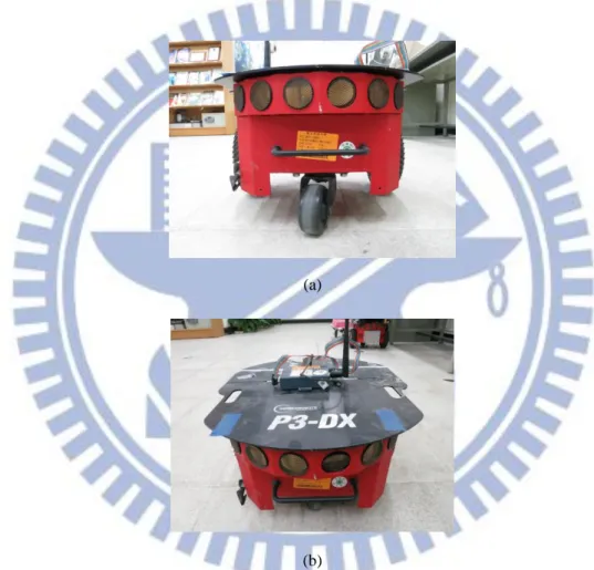
In the vehicle system, the Pioneer 3-DX as mentioned is shown is Figure 2.2, which has a 44cm×38cm×22cm aluminum body with two 19cm wheels and a 7cm caster. It can reach a speed of 5.76 kilometer per hour on flat floors; has the maximum rotation speed of 300 degrees per second; and can climb up an incline with the largest slope of 30 degrees. Moreover, the vehicle has sixteen ultrasonic sensors. They are

three 12V rechargeable lead-acid batteries and can run 18-24 hours if the batteries are fully charged initially. Furthermore, the vehicle is equipped with an odometer which records the pose of the vehicle, including the position and the orientation with respect to its initial pose, for each navigation cycle. The odometer provides also the readings of the vehicle speed, the battery voltage, etc.

(a)

(b)

(c)

Figure 2.1 Three different views of the used hardware architecture, which includes a vehicle and a stereo camera. (a) A 45o view. (b) A front view. (c) A side view.

The second part of the system hardware is the camera system. It is a two-mirror omni-camera which consists of one perspective camera, one lens, and two reflective mirrors of different sizes, all integrated into a single structure. A picture of the camera

2.4. The camera is of the model ARCAM-200SO, which is produced by ARTRAY Company with the size of 33mm×33mm×50mm and the resolution of 2.0M pixels. The detailed specifications of the camera are listed in Table 2.1. The lens is produced by Sakai Co. and has a variable focal length of 6-15mm. The two reflective mirrors are produced by Micro-Star International Co. The structure of the camera system will be described in more detail in the next section.

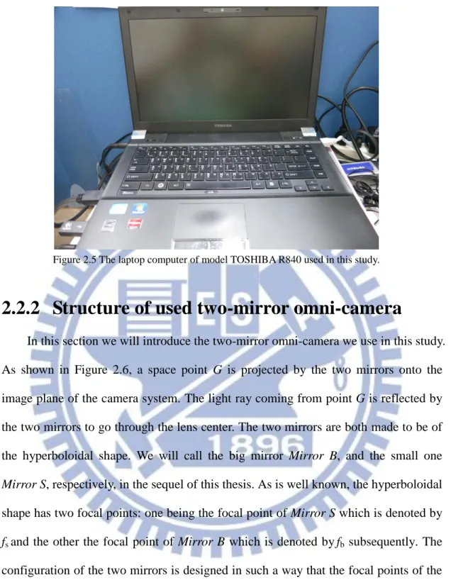
In the control system, we utilize a laptop computer as the main unit. It is of model R840 produced by TOSHIBA Computer Inc. as shown in Figure 2.5. We use an RS-232 to connect the laptop computer and the autonomous vehicle and use a USB to

(a)

(b)

Figure 2.2 The Autonomous vehicle, Pioneer 3-DX, produced by MobileRobots Inc., used in this study. (a) A back view. (b) A front view.

in Table 2.2.

(a) (b)

Figure 2.4 The used camera and lens. (a) The camera of model Arcam-200so produced by ARTRAY Co. (b) The lens produced by Sakai Co.

Table 2.1 The specification of Arcam-200so.

Size 33mm×33mm×50mm

CMOS Size 1/2” (6.4 × 4.8mm)

Mount C-mount

Max resolution 2.0 M pixels

Frame per second with max resolution 8 fps

Figure 2.5 The laptop computer of model TOSHIBA R840 used in this study.

2.2.2 Structure of used two-mirror omni-camera

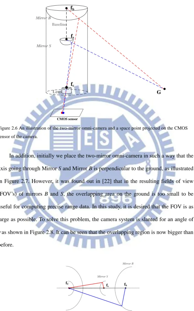
In this section we will introduce the two-mirror omni-camera we use in this study. As shown in Figure 2.6, a space point G is projected by the two mirrors onto the image plane of the camera system. The light ray coming from point G is reflected by the two mirrors to go through the lens center. The two mirrors are both made to be of the hyperboloidal shape. We will call the big mirror Mirror B, and the small one Mirror S, respectively, in the sequel of this thesis. As is well known, the hyperboloidal

shape has two focal points: one being the focal point of Mirror S which is denoted by fs and the other the focal point of Mirror B which is denoted byfb subsequently. The

configuration of the two mirrors is designed in such a way that the focal points of the two mirrors are located at an identical point which is just the lens center fc of the

camera. Besides, the distance from the mirror center of Mirror B to the mirror center of Mirror S has a length of 20 cm according to our manual measurement in this study. We call it the baseline. The detailed information of the two hyperboloidal-shaped

Table 2.2 Specification of the laptop computer. CPU Intel Sandy Bridge Core i5-2410M 2.3GHz

RAM 4G DDR 1333MHz

GPU AMD Radeon HD 6450 /1024MB

HDD Size 640 GB

Table 2.3 Specifications of the used two hyperboloidal-shaped mirrors.

Radius Parameter a Parameter B

Mirror S 2 cm 2.41 cm 4.38 cm

Mirror B 12 cm 11.46 cm 9.68 cm

In spite of having two focal points, the hyperboloidal shape has another property as shown Figure 2.7: if a light way goes through one of the focal point, it will be reflected to go through the other focal point by the mirror. This property has been utilized to construct the omni-camera in a previous study [22] . According to this property, a space point G will first go into the centers of the two mirrors, then reflected by the mirrors to go through the lens center fc , and finally projected onto the

CMOS sensor of the camera. Therefore, we have two distinct image points corresponding to the single space point G. Based on such a phenomenon, we can compute the range data of G. The detail will be described later in this chapter.

In addition, initially we place the two-mirror omni-camera in such a way that the axis going through Mirror S and Mirror B is perpendicular to the ground, as illustrated in Figure 2.7. However, it was found out in [22] that in the resulting fields of view (FOV’s) of mirrors B and S, the overlapping area on the ground is too small to be useful for computing precise range data. In this study, it is desired that the FOV is as large as possible. To solve this problem, the camera system is slanted for an angle of as shown in Figure 2.8. It can be seen that the overlapping region is now bigger than before. Mirror B Mirror S fb fs fC fb fs fc G CMOS sensor Mirror B Mirror S Lens Baseline

Figure 2.6 An illustration of the two-mirror omni-camera and a space point projected on the CMOS sensor of the camera.

Mirror B Mirror S (a) Mirror B Mirror S _γ (b)

Figure 2.8 Two different placements of the two-mirror omni-camera on the vehicle and the region of overlapping. (a) The optical axis going through the two mirrors is parallel to the ground. (b) The optical axis through the two mirrors is slanted up for an angle of.

2.2.3 Software configuration

MobileRobots Inc., which provides the autonomous vehicle for use in this study, provides an application interface, called ARIA (Advanced Robotics Interface Application), for the user to control the vehicle. The ARIA is an object-oriented interface which can be used under the Linux or Win32 operating system using the C++ language. Therefore, we can use the ARIA to communicate with the embedded sensor system in the vehicle and obtain the information which the vehicle offers to control the position of the vehicle.

For the camera system, the ARTRAY provides a tool which is called Capture Module Software Developer Kit (SDK). It is an object-oriented interface and its

application interface is written in several computer languages like C, C++, VB.net, C#.net and Delphi. We use the SDK to capture image frames with the camera and

system, we use Borland C++ Builder 6 with updated pack 4 on the Windows XP operating system. The Borland C++ Builder 6 is a GUI-based interface development environment (IDE) software. It is convenient for us to provide a friendly interface for the user.

2.3 3D Data Acquisition by the

Two-mirror Omni-camera

2.3.1 Review of imaging principle of two-mirror

omni-camera

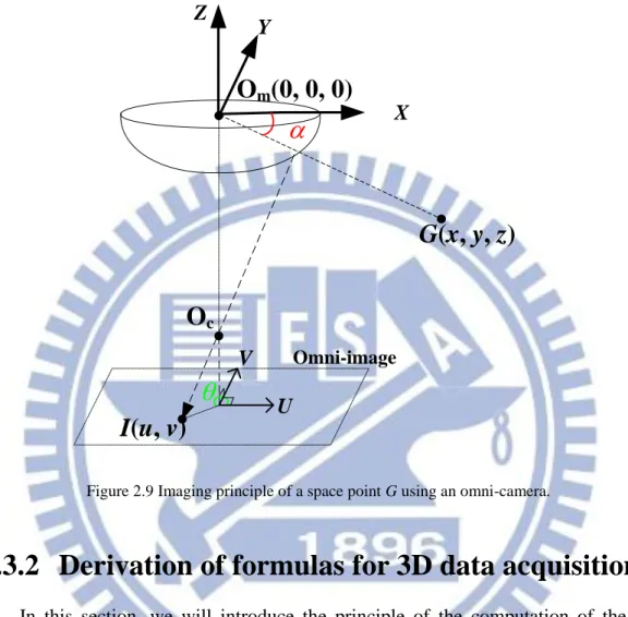
In this section, we review the two-mirror omni-camera proposed in Huang and Tsai [22] and used in this study, as well as the formulas for range data computation using images captured by such a camera system. First, we review the image projection principle of an omni-camera. As shown in Figure 2.9, we use the two coordinate systems, the image coordinate system (ICS) and the camera coordinate system (CCS), to illustrate the principle of imaging process. The image coordinate system is a two-dimensional U-V coordinate system and the other is a three-dimensional X-Y-Z coordinate system. The origin of the first one is the center of the omni-image, and the second is the focal point of the hyperboloidal-shaped mirror. As mentioned previously, a light ray G at (x, y, z) in the CCS go through the focal point of the hyperboloidal-shaped mirror Om, and reflected by the mirror. Then, it goes through the

other focal point at center of lens Oc. Finally it is projected onto an image point I on

the omni-image plane at (u, v). As a result, each image point in an omni-image can be specified by an elevation angle and an azimuth angle After the azimuth angle

space point G.

O

(0, 0, 0)

G(x, y, z)

O

I(u, v)





Figure 2.9 Imaging principle of a space point G using an omni-camera.

2.3.2 Derivation of formulas for 3D data acquisition

In this section, we will introduce the principle of the computation of the 3D range data. We will now define the direction of the camera coordinate system (CCS) CCSlocal in Figure 2.10. As seen in the figure, two light rays from G in CCSlocal go

through the center of Mirror S and that of Mirror B, and1 and2 are the elevation

angles, respectively. The points Os, O_b, G form a triangle O_sO_bG which is illustrated

in Figure 2.11. We know the distance from Os to Ob by manual measurement which is

called the baseline in the last section. We can derive the following equations by the law of sines based on the geometry:

sin(90o _b) sin( _b)

d b



   

  . (2.1)

Then, we can calculate accordingly the baseline as follows:

sin(90 ) sin( ) o b b b d         =

 









Figure 2.10 The cameras coordinate systemCCS_local, and a space point G projected on the omni-image acquired by the two-mirror omni-camera.

Then, we want to know the azimuth angles of the two light rays. According to the property of rotational invariance of the omni-image, these two azimuth angles actually are equal, which we denote by . From Figure 2.12, the azimuth  in the ICS can be computed by using the image coordinates (u1, v1) of G according to the

Ob Mirror B Mirror S

α

d

d

-

b

Figure 2.11 An illustration of the relation between a space point G and the two mirrors in the used camera. (a) A side view of G projected onto the two mirrors. (b) A triangle ObOsG used in deriving

3D data. 1 1 2 2 2 2 1 1 1 1 sin u ; cos v u v u v       ; 1 1 1 1 2 2 2 2 1 1 1 1 sin ( u ) cos ( v ) u v u v  _  _    . (2.3)

After obtaining the distance d by Equation (2.2) and the azimuth angle θ by Equation (2.3), we can compute the position of G, namely, the global coordinates (X, Y, Z), in

local

CCS by the following equations:

X ＝ d × cosαa × sinθ,

Y ＝ d × cosαa × sinθ,

d θ Y Z U V Oc Os Baseline G(X , Y , Z) Ob ICS X X Y _Z CCSlocal

Figure 2.12 An illustration of a space point G at coordinates (X, Y, Z) in CCS_local.

As mentioned previously, the camera system we use in this study is not set parallel to the ground so as to enlarge the overlapping area of both mirrors; instead, it is slanted up for an angle of  as shown 2.13. It is desired that the Z-axis of CCS_local

could be parallel to the ground. We define another camera coordinate system CCS which coincides with CCS_local except the Z-axis is be elevated by an angle of 

Finally, we can use a rotational matrix R to represent the G in the CCS by the following equations: 1 0 0 0 cos( ) sin( ) 0 sin( ) cos( ) R         _    _       ; (2.5) ' 1 0 0 ' 0 cos( ) sin( ) ' 0 sin( ) cos( ) X X Y Y Z Z             _{   }                        . (2.6)

2.4 System Operation Processes

2.4.1 Learning process

In the learning process, it is important for the autonomous vehicle to “learn” the selected path and conduct navigation automatically. In this section, we will describe the information which the vehicle should “memorize” in detail. Initially, the vehicle has to record where the selected path in the outdoor environment is. For this study, the experimental place is a sidewalk in the campus of National Chiao Tung University. Because the vehicle navigates on the sidewalk, we can take the advantage of the sidewalk curb to implement a “curb following” function for vehicle guidance. It also

helps the vehicle to calibrate the odometer precisely. In addition, the lighting condition is a concern in the outdoor environment. So, the different location information must be recorded in the navigation path.

Moreover, another odometer calibration method adopted in this study is via landmark detection. By this method, the trainer can choose the landmarks which should be learned in the selected path, and decide where to localize the vehicle by the learning landmarks. Next, landmark detection is accomplished by a space line

Z’ Y Z X CCS   CCS’ X’ Y’

detection technique in this study, which is described in Chapter 5. After collecting enough information of the learned landmark, some parameters for landmark detection and the position of each landmark can be recorded.

To facilitate the user to learn navigation paths, a user learning interface is designed for the trainer. They may use it to control the autonomous vehicle to construct the navigation path. Furthermore, after the vehicle detects a landmark, we provide a semi-automatic learning process to adjust the parameters which we sat initially for the trainer to deal with some varying conditions of the environment. Also, the trainer should establish the navigation rules in advance for the vehicle to follow in the navigation process.

At last, after leading the autonomous vehicle to the destination, the learning process is finished. The learned information is organized into a learned path which is composed of several path nodes with guidance parameters. We finally acquire the navigation path map which combined the landmark information and the environment information, and store in the disk. The entire learning process proposed in this study is shown in Figure 2.14.

2.4.2 Navigation process

In the navigation process, the autonomous vehicle can analyze the current location using various stored information obtained in the learned process and navigate to the next node on the learned path. The entire navigation process proposed in this study is shown in Figure 2.15.

In general, the autonomous vehicle analyzes the current environment node by node to navigate to the goal according to the learned information data retrieved from

too light, the vehicle can be “confused” by the image we got from the camera system. According to the learning environment information, the system was designed to be able to adjust the exposure of the camera dynamically if necessary.

Besides, the autonomous vehicle always checks if any obstacle exists in front of the vehicle. As soon as an obstacle is found and checked to be too close to the vehicle, a procedure of collision avoidance is started automatically to perform collision avoidance. In addition, if the vehicle gets a node of “landmark detection,” the

Learning of landmarks Learning of

environment Learning of navigation path

Learning interface Start of learning Establish navigation rules Establish landmark deteciton rules Manual navigate vehicle Detect landmarks End of learning Automatic sidewalk following Create navigation map Vehicle odometer Landmark localization Learning information Map information Vehicle navigation information Landmark location analysis Landmark information Environment information

autonomous vehicle will adjust the detection pose and load the parameters for landmark detection. If a landmark is found successfully, the landmark’s position is used to modify the odometer of the vehicle; if not, some strategy of recovering the landmark are started, such as changing the parameters for landmark detection or changing the pose of the vehicle to detect landmark successfully.

Vehicle navigation loop Vehicle localization procedure Obstacle avoidance loop

Start of navigation Sidewalk feature extraction Landmark feature extraction Landmark position localization End of navigation Read a new node and navigation initialization Sidewalk following? Arriving at a node? Initialization to detect landmark Arrive at terminal node? obstacle detected? Localize obstacle Yes No No Yes Yes No Yes No Vehicle localization? Yes No Blind navigation Navigation by sidewalk following Modify vehicle location Collision avoidance Map information Landmark information Landmark found? Yes Remedy of landmark detection No

Chapter 3

Learning Strategy for Automatic

Navigation

3.1 Introduction

The purpose of the learning process for the proposed machine guide dog system is to create a path on a sidewalk to guide a blind person to a selected destination. Before starting to learn a path, we have to do some works. First, at first we have to choose some landmarks for vehicle localization. Then, we have to calibrate the camera system. The third task is to infer some guidance parameters. At last, we should adopt a learning strategy to learn certain information about each selected landmark.

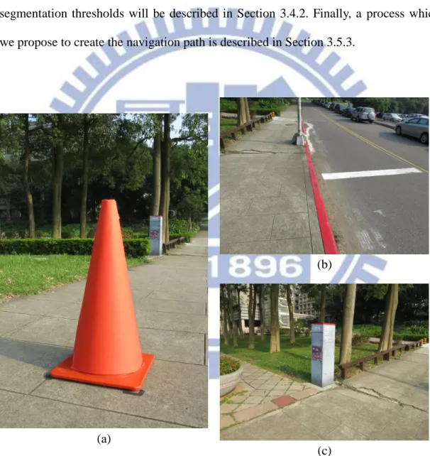
3.1.1 Selected landmarks in outdoor environments

for this study

When the vehicle is in the navigation process, mechanic errors usually will accumulate up to cause imprecise odometer readings of the vehicle location and orientation. To solve such problems, in this study we adopt the approach of vehicle localization using landmarks. For this purpose, some objects should be selected as

landmarks at first to conduct the localization work. Chou and Tsai [23] detected the light pole and the hydrant to localize the vehicle. In this study, we select instead some other natural and artificial objects as landmarks, which are commonly seen on sidewalks. Specifically, we select two types of natural landmarks, tree trunk and lawn

the same purpose are three types of artificial landmarks, namely, signboard, traffic cone, and stop line on roads, as shown in Figure 3.2. With more types of landmarks so

selected, we can have more information along the way for localization, and we can then guide the autonomous vehicle to the destination more reliably. The detailed proposed methods for vehicle localization using landmarks will be introduced later in Chapters 5 and 6. In this chapter, we discuss the learning process for these landmarks and other information.

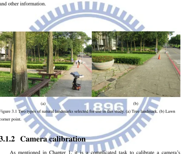
3.1.2 Camera calibration

As mentioned in Chapter 1, it is a complicated task to calibrate a camera’s intrinsic and extrinsic parameters. A space-mapping technique [24], called pano-mapping, is adopted instead in this study to “calibrate” the two-mirror omni-camera system used in this study. We will introduce the adopted technique in Section 3.2.

(a) (b)

Figure 3.1 Two types of natural landmarks selected for use in this study. (a) Tree landmark. (b) Lawn corner point.

To navigate in outdoor environments, a trainer of the proposed vehicle system should guide the system to learn and record some parameters of the sidewalk environment for use in the navigation process. The parameters to be learned in this study include image segmentation thresholds and some other environment parameters. The proposed technique for learning the adopted environment parameters will be described in Section 3.4.1. Also, the proposed method for learning the used image segmentation thresholds will be described in Section 3.4.2. Finally, a process which we propose to create the navigation path is described in Section 3.5.3.

(a)

(b)

(c)

Figure 3.2 Three artificial landmarks used in this study. (a) Tree landmark. (b) Road stop line landmark. (c) Signboard landmark.

3.2 Camera Calibration by

Space-mapping Approach

To calibrate the camera system used in this study, we use the pano-mapping technique proposed by Jeng and Tsai [24]. Specifically, it is desired to establish a pano-mapping table to record the relations between the locations of image points and

those of the corresponding real-world points. For this, as mentioned in Chapter 2, we assume first that a light ray going through a world-space point P with the elevation angle α and the azimuth angle θ is projected onto a specific point p at coordinates (u, v) in the omni-image. The pano-mapping table specifies the relation between the

coordinates (u, v) of the pixel p in the image and the azimuth-elevation angle pair ( of the corresponding world-space point P. We construct the pano-mapping table once, and the table can be looked up to retrieve 3D information forever. Specifically, we establish two pano-mapping tables for Mirrors S and B, respectively, in the camera system used in this study. The details are described in the following algorithm.

Algorithm 3.1 Construction of pano-mapping tables.

Input: two sets of six landmark point pairs (pi, Pi) and (qj, Qj) selected in advance

manually where pi and qi are points in an omni-image I and Pi and Qj are the

corresponding points in the world space.

Output: two pano-mapping tables of dimension M× N for Mirrors B and S.

Steps.

Step. 1. Let the six known image pixels pi be located at coordinates (ui, vi,) in the

Step. 2. Similarly let the six known image pixels qj be located at coordinates (Uj, Vj,)

in the Mirror S region in omni-image I and the six corresponding known world-space points Qj be at coordinates (Xj, Yj, Zj) in the camera coordinate

system, where j = 1, 2, …, 6.

Step. 3. Calculate the radial distances ri and Rj in the image plane from the image

pixels pi and qj to the image center, respectively, by the following equations:

2 2 2 2

; .

i i i i i i

r  u u R  U V (3.1)

resulting in six pairs of radial distances ri and Ri for Mirrors S and B,

respectively.

Step. 4. Calculate the elevation angles αi and βi for the world-space points Pj and Qj,

respectively, by the following equations:

2 2 2 2 1 1 tan ( / ); tan ( / ) i zi xi yi i Zi Xi Yi  _  _  _  _ , (3.2)

resulting in sixpairs of elevation angles for Mirrors S and B, respectively. Step. 5. Under the assumption that the surface geometries of Mirrors S and B are

radially symmetric in the range of 360 degrees, use two radial stretching functions, denoted as fS and fB, to describe the relationship between the radial

distances ri and the elevation angles αi as well as that between Rj and βj,

respectively, by the following equations where i = 1, 2, …, 6:

1 2 3 4 5 0 1 2 3 4 5 ( ) i S i i i i i i r  f    s s   s   s   s   s  ; 1 2 3 4 5 0 1 2 3 4 5 ( ) i B i i i i i i R  f    b b   b   b   b   b  . (3.3)

Step. 6. Solve the above 6-th degree polynomial equations for fA and fB by the uses of

Step 4 as well as a numerical method to obtain the coefficients a0 through a5

and b0 through b5.

Step. 7. By the use of the function fB with the known coefficients b0 through b5,

construct a pano-mapping table TB for Mirror B in a form as that shown in

Table 3.1(a) according to the following rule:

for each world-space point Pij with the azimuth-elevation pair (θi, j),

compute the corresponding image coordinates (uij, vij) by the following

equations:

cos ; sin

ij j i ij j i

u  r  v  r  . (3.4)

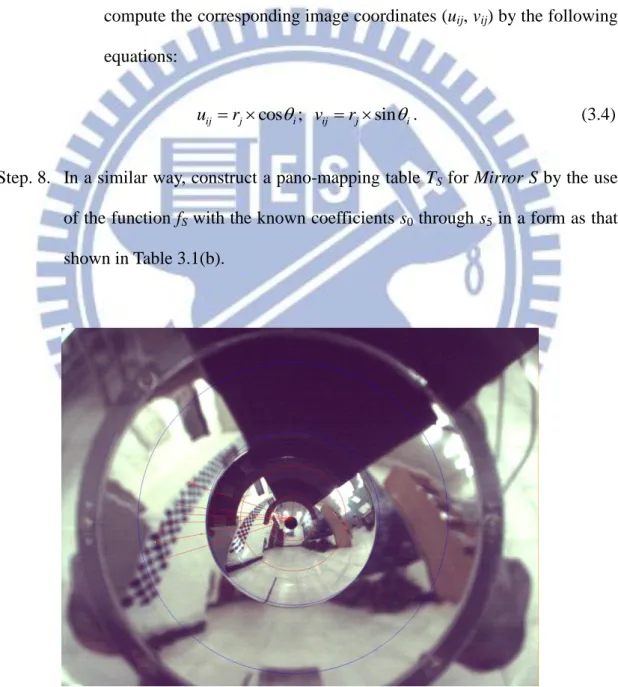
Step. 8. In a similar way, construct a pano-mapping table TS for Mirror S by the use

of the function fS with the known coefficients s0 through s5 in a form as that

shown in Table 3.1(b).

Table 3.1 Two pano-mapping tables used for the two-mirror omni-camera used in this study. (a) Pano-mapping table used for Mirror B. (b) Pano-mapping table used for Mirror S.

1 2 3 4 … S 1 (u11, v11) (u21, v21) (u31, v31) (u41, v41) … (uS1, vS1)  2 (u12, v12) (u22, v22) (u32, v32) (u42, v42) … (uS2, vS2)  3 (u13, v13) (u23, v23) (u33, v33) (u43, v43) … (uS3, vS3)  4 (u14, v14) (u24, v24) (u34, v34) (u44, v44) … (uS4, vS4)  … … … …  T (u1T, v1T) (u2T, v2T) (u3T, v3T) (u4T, v4T) … (uST, vST) (a) 1 2 3 4 … M 1 (u11, v11) (u21, v21) (u31, v31) (u41, v41) … (uM1, vM1) 2 (u12, v12) (u22, v22) (u32, v32) (u42, v42) … (uM2, vM2) 3 (u13, v13) (u23, v23) (u33, v33) (u43, v43) … (uM3, vM3) 4 (u14, v14) (u24, v24) (u34, v34) (u44, v44) … (uM4, vM4)  … … … … N (u1N, v1N) (u2N, v2N) (u3N, v3N) (u4N, v4N) … (uMN, vMN) (b)

3.3 Coordinate Systems

In this study, the following four coordinate systems are used to describe the vehicle location and the navigation environment. The coordinate systems are illustrated in Figure 3.4 and defined in the following.

(1). Image coordinate system (ICS, denoted as u-v): The origin OI of the image

coordinate system is located at the center of the image plane, and the u-v plane coincides with the image plane.

(2). Camera coordinate system (CCS, denoted as X-Y-Z): The origin OC of the CCS is

located at the focal point of Mirror B. The X-Z plane is parallel to the ground and the Y-axis is perpendicular to the ground.

(3). Vehicle coordinate system (VCS, denoted as VX-VY): The origin OV of the vehicle

coordinate system is located at the center of the autonomous vehicle, and the VX-VY plane coincides with the image plane.

(4). Global coordinate system (GCS, denoted as GX-GY): The origin OG of this system

is always set at the start position of the vehicle in the navigation path, and the G -G plane coincides with the ground.

When the vehicle is moving in the navigation session, we have to know the relationships among the coordinate systems. It is advantageous to utilize an odometer to localize the vehicle position in the GCS, though the odometer readings are not very accurate all the time. At the beginning of each navigation process, the VCS and CCS follow the vehicle, and the VCS coincides with the GCS. After the vehicle moves for a short distance, as illustrated in Figure 3.5, and stops at a position V at world coordinates (Cx, Cy) with a rotation angle θ, we can derive the coordinate

transformation between the coordinates (VX, VY) of the VCS and the coordinates (GX,

GY) of the GCS by the following equations:

cos sin sin cos x x x y y y G V C V C G      _     _                _{. (3.5)} Omni-image

u

v

O

G

G

Figure 3.4 Four coordinate systems used in this study. (a) The ICS. (b) The CCS. (c) The VCS. (d) The GCS.