渦輪等化及渦輪碼在MIMO-OFDM系統上之實現

(1)

國立交通大學

電信工程學系碩士班

碩士論文

渦輪等化及渦輪碼在

MIMO-OFDM

系統上之實現

Turbo Equalization And Turbo coding for MIMO-OFDM

System

研究生：林育丞

指導教授：吳文榕博士

(2)

渦輪等化及渦輪碼在

MIMO-OFDM 系統上之實現

Turbo Equalization and Turbo coding for MIMO-OFDM

System

研究生：林育丞 Student：Yu-Cheng Lin

指導教授：吳文榕博士 Advisor：Dr. Wen-Rong Wu

國立交通大學

電信工程學系碩士班

碩士論文

A Thesis

Submitted to Department of Communication Engineering

College of Electrical and Computer Engineering

National Chiao-Tung University

in Partial Fulfillment of the Requirements

for the Degree of

Master of Science

In

Communication Engineering

July 2007

Hsinchu, Taiwan, Republic of China

中華民國九十六年七月

(3)

渦輪等化及渦輪碼在

MIMO-OFDM 系統上之實現

研究生：林育丞指導教授：吳文榕教授

國立交通大學電信工程學系碩士班

摘要

在這篇論文中，我們著重在多輸入多輸出(MIMO)-正交分頻多工(OFDM)系統的外部接收機設計。外部接收機主要包括軟性位元產生器與錯誤更正碼解碼器，一般將這兩部分視為獨立，但依此無法達到最佳效能。在第一部分，我們研究渦輪等化(Turbo Equalization) 在多輸入多輸出(MIMO)-正交分頻多工(OFDM)系統中的應用。此方法藉由遞迴的方式來結合軟性位元反對映與錯誤更正碼解碼。然而，位元交錯調變碼(BICM)依舊將錯誤更正碼以及調變視為獨立，並沒有利用到多輸入多輸出(MIMO)架構。而頻帶交錯調變碼(TICM)可用來解決這個問題。在第二部分，我們提出在渦輪碼(Turbo coding)在頻帶交錯調變碼(TICM) 上的應用。在 802.11n 系統下，模擬證明渦輪等化以及渦輪碼結合頻帶交錯調變碼的效能均優於傳統的做法。

(4)

Turbo Equalization and Turbo coding for MIMO-OFDM System

Student:

Yu-Cheng

Lin

Advisor:

Dr.

Wen-Rong

Wu

Department of Communication Engineering

National Chiao-Tung University

Abstract

In this thesis, we focus on the outer receiver design for multiple-input-multiple output (MIMO) OFDM systems. The outer receiver mainly consists of a soft-bit demapper and an outer code decoder. The conventional approach considers these two devices separately, and cannot achieve true optimum performance. In the first part of the thesis, we study the application of turbo equalization technique in MIMO-OFDM systems. Using this approach, we can combine demapping and decoding in an iterative way. The conventional communication system often uses the bit-interleaved-coding modulation (BICM) scheme. However, the BICM scheme treats coding and modulation separately, and does not exploit the MIMO structure constraint. Tone-interleaved- coding-modulation (TICM) has been proposed to solve the problem. However, only the

convolution code was considered. In the second part of the thesis, we propose to use the turbo code in the TICM scheme. Simulations with the IEEE 802.11n systems show that both the turbo equalization and the TICM schemes can significantly outperform conventional approaches.

(5)

誌謝

本篇論文得以順利完成，首先要特別感謝我的指導教授吳文榕博士，在

課業學習與論文研究上不厭其煩的引導我正確的方向。

另外，我要感謝許兆元學長、李俊芳學長與楊華龍學長等在研究上不吝指

導，且同時感謝寬頻傳輸與訊號處理實驗室所有同學與學弟妹們的幫忙，以及

昭曄和健甫無私的提供資源上的協助。特別感謝沈士琦學長，在工作百忙之餘

仍撥冗與我討論，並給我許多建議。最後感謝我家人以及佳盈，給予我在精神

上最大的鼓勵與支持，使得我可以順利地完成碩士學位。

(6)

List of Tables

Table 2-1: The primary parameters in the TGn Sync proposal ... 5 Table 2-2: Model parameters for LOS/NLOS conditions ... 6 Table 2-3: Path loss model parameters ... 7

(9)

List of Figures

Fig. 2-1: The block diagram of the transmitter in the TGn Sync proposal... 4

Fig. 2-2: The block diagram of the MIMO-OFDM transmitter for BICM... 10

Fig. 2-3: The block diagram of the MIMO-OFDM receiver for BICM ... 10

Fig. 2-4: The block diagram of the SISO-OFDM transmitter for BICM ... 13

Fig. 2-5: The block diagram of the SISO-OFDM receiver using the MMSE equalizer for BICM ... 13

Fig. 2-6: Partitions of the 16-QAM constellation... 13

Fig. 2-7: The block diagram of the MIMO-OFDM receiver using the LSD detector for BICM... 14

Fig. 2-8: LSD with the given radius of the sphere... 16

Fig. 2-9: Diagram of turbo processing for the OFDM-MIMO system... 20

Fig. 2-10: Recursive calculating of α in trellis diagram ... 23

Fig. 2-11: Recursive calculating of β in trellis diagram ... 24

Fig. 2-12: Performance comparison of soft+BCJR and turbo scheme (20MHz, 2x2, 16-QAM, channel-B, perfect-channel)... 29

Fig. 2-15: Performance comparison of soft+BCJR and turbo scheme (20MHz, 2x2, 16-QAM, channel-D, perfect-channel)... 30 Fig. 2-16: Performance comparison of soft+BCJR and turbo scheme (20MHz, 4x4,

(10)

16-QAM, channel-D, perfect-channel)... 31

Fig. 2-17: Performance comparison of soft+BCJR and turbo scheme (20MHz, 4x4, 64-QAM, channel-D, perfect-channel)... 31

Fig. 2-18: Performance comparison of soft+BCJR and turbo scheme (20MHz, 2x2, 16-QAM, channel-B, estimated-channel)... 32

Fig. 2-21: Performance comparison of soft+BCJR and turbo scheme (20MHz, 4x4, 16-QAM, channel-D, estimated-channel) ... 34

Fig. 3-1: The block diagram of the MIMO-OFDM transmitter for TICM-T ... 38

Fig. 3-2: The turbo encoder for TICM-T... 40

Fig. 3-3: The block diagram of the MIMO-OFDM receiver for TICM-T ... 41

Fig. 3-4: The iteration loop of the TICM-T... 43

Fig. 3-5: The block diagram of the MIMO-OFDM transmitter for BICM-T... 48

Fig. 3-6: The block diagram of the MIMO-OFDM receiver using the LSD for BCIM-T ... 48

Fig. 3-7: Performance comparison of BICM-T, and TICM-T (20MHZ, 4X4 16-QAM, channel B, estimated-channel)... 50

(11)

Fig. 3-8: Performance comparison of BICM-T, and TICM-T (20MHZ, 4X4 16-QAM, channel B, estimated-channel)... 50

(12)

Chapter 1 Introduction

Turbo equalization [1] [2] is a powerful mean to perform joint equalization and decoding, when considering coded data transmission over time dispersive channels. It can significantly improve the equalization result. The association of the code and the discrete-time equivalent channel (separated by an interleaver) is seen as the serial concatenation of two codes. The turbo principle can then be used at the receiver: performances are improved through an iterative exchange of extrinsic information between a soft-in/soft-out (SISO) equalizer and a SISO decoder. Classically, these SISO modules are implemented using conventional a posteriori probability (APP) algorithms based on [3].

Orthogonal frequency division multiplexing (OFDM), proposed by Salzberg in 1967 [6], is known to have high spectrum efficiency and good resistance against multi-path interference. Moreover, duplexing and multiple accesses can be easily implemented with a frequency division manner. One way to further enhance rates on a scattering-rich wireless channel is to use multiple transmit and receive antenna (MIMO) structure. However, the MIMO structure will induce the interference between different transmit antennas. A simple solution for the problem is to use a zero-forcing (ZF) or minimum-mean-squared-error (MMSE) equalizer to suppress the interference, and then convert the MIMO system into multiple SISO systems. Since the noise becomes correlated after the equalization, conventionally used SISO soft-demappers are not optimal. The optimum MIMO soft-demapper is known to require very high computational complexity, even higher than maximum likelihood (ML) estimator. An efficient algorithm named list sphere decoding (LSD) was proposed [5] to solve the problem. It has been shown that the LSD algorithm can significantly reduce the computational complexity, while having near optimum performance.

(13)

The bit interleaved coded modulation (BICM) scheme, originally proposed by Zehavi [6], inserts a bit-level interleaver between the encoder and the QAM mapper to reduce the bursty error problem, improving the error correction capability of the forward-error correction (FEC) coder. As a result, the BICM scheme is popularly applied in fast fading channel environments. In orthogonal frequency division multiplexing (OFDM) systems, subcarriers within same coherent bandwidth can experience deep fades even the channel is non-fading. The BICM scheme is then useful in this scenario.

In addition to the LSD algorithm, there is another way improving the performance of MIMO-OFDM systems when the BICM is used. The MIMO structure introduces interference between data transmitted in different antenna. Thus, the effect can be been as the result of an additional coder. Combining with the original FEC coder, we can then apply the turbo equalization. Using the turbo principle, we can improve the detection performance by exchanging the information between the MIMO soft-demapper and the channel decoder. This problem has been considered in [5] and the result show significant performance improvement.

To develop the next generation of wireless local area networks (WLAN), IEEE announced an 802.11n Task Group (TGn) in January 2004. The target data rate for the new standard have a theoretical bound of 540Mbit/s. In other words, it will be 100 times faster than 802.11b, or 10 times faster than 802.11a/11g. The modulation of 802.11n uses the MIMO-OFDM and BICM techniques such that the throughput can be significantly increased and the channel fading effect can be minimized. In the first part of this thesis, we will investigate turbo equalization in IEEE 802.11n system. We will use the channel models suggested by the standard to evaluate the performance of turbo equalization. The LSD method, mentioned above, will be used to obtain the MIMO soft-demapping results.

(14)

in [11], uses the symbol block as a unit for interleaving, instead of bits. With this structure, the detection symbols in the received symbol vector (after the MIMO channel) can have a trellis relationship. As a result, the detection performance can be improved. However, since the interleaving is conducted in the symbol block level, the resistance to busty error is reduced. Simulation results show that when the delay spread of the channel is short, TICM can have much better performance, and when the delay spread of the channel is long, TICM does not have significant advantages. Note that only convolutional coders are considered in [11]. In the second part of the thesis, we then propose to apply the turbo code in TICM. Since there is an interleaver between two component decoders, the bursty error problem can then be reduced. It is expected that TICM with a turbo code can outperform BICM with the same turbo code.

The rest of this thesis is organized as follows: In Chapter 2, we review IEEE802.11n systems, and the conventional demodulation method for the MIMO-OFDM system with BICM, including the MMSE equalizer, the soft-bit demapper, and the LSD detector. Also, we will describe how to apply turbo equalization in MIMO-OFDM system. In Chapter 3, we describe the proposed TICM scheme and its optimal demodulation method. Finally, we draw some conclusions and outline future works in Chapter 4.

(15)

Chapter 2 Turbo Equalization in MIMO-OFDM

Systems

In MIMO-OFDM systems with BICM, we can treat the MIMO channel as an inner code and the FEC coder as an outer code, and use an “iterative decoding” technique [5] to approach the optimum performance of joint equalization and detection. This is commonly called turbo equalization. In this chapter, we will first review IEEE 802.11n systems, and outline the conventional MIMO-OFDM receiver. Then, we will discuss the LSD detector and MIMO soft-demapper. Finally, we will describe turbo equalization in MIMO-OFDM systems, and the corresponding application in IEEE802.11n systems.

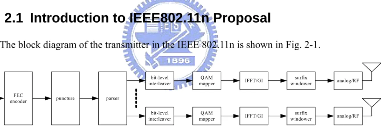
2.1 Introduction to IEEE802.11n Proposal

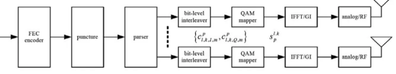
The block diagram of the transmitter in the IEEE 802.11n is shown in Fig. 2-1.

FEC

encoder puncture parser

bit-level

interleaver mapperQAM IFFT/GI bit-level interleaver QAM mapper IFFT/GI analog/RF analog/RF surfix windower surfix windower

Fig. 2-1: The block diagram of the transmitter in the TGn Sync proposal

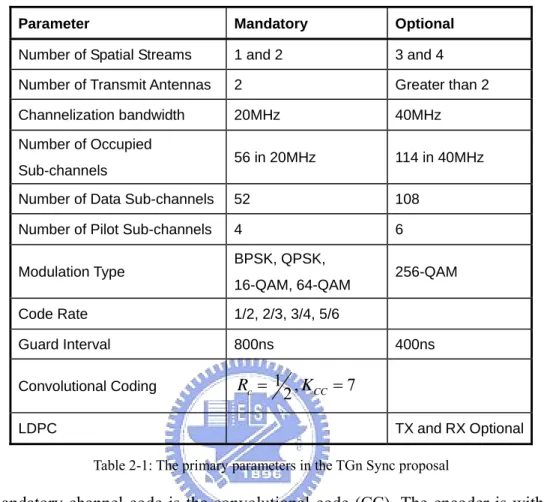
The mandatory number of spatial streams is two and the mandatory channelization bandwidth is 20MHz. The proposal also utilizes optional techniques such as four spatial streams, and 40MHz channelization bandwidth. Table 2-1 shows the primary parameters in the proposal.

(16)

Parameter Mandatory Optional Number of Spatial Streams 1 and 2 3 and 4

Number of Transmit Antennas 2 Greater than 2 Channelization bandwidth 20MHz 40MHz Number of Occupied

Sub-channels 56 in 20MHz 114 in 40MHz Number of Data Sub-channels 52 108

Number of Pilot Sub-channels 4 6 Modulation Type BPSK, QPSK,

16-QAM, 64-QAM 256-QAM Code Rate 1/2, 2/3, 3/4, 5/6

Guard Interval 800ns 400ns Convolutional Coding Rc =1 ,₂ KCC =7

LDPC TX and RX Optional

Table 2-1: The primary parameters in the TGn Sync proposal

The mandatory channel code is the convolutional code (CC). The encoder is with K_CC = 7

andR_c = 1₂, where K_CC represents the constraint length of the CC encoder, and R represents _c

the code rate. The encoded output is then punctured, according the required data rate, and then parsed to multiple spatial streams. To have the frequency diversity gain and reduce the spatial correlation of the MIMO channel, the binary data is interleaved by the size of OFDM symbol and

then mapped into 2M_{-quadrature amplitude modulation (QAM) symbols, which are used to}

modulate data carriers in subchannels. Each OFDM symbol allocates N_sd =52 subchannels for

data transmission.

2.2 MIMO Channel Model

(17)

for these channel models can be described as follows.

(Channel-A). a typical office environment, non-line-of-sight (NLOS) conditions, and 50 ns rms delay spread

(Channel-B). a typical large open space and office environments, NLOS conditions, and 100 ns rms delay spread

(Channel-C). a large open space (indoor and outdoor), NLOS conditions, and 150 ns rms delay spread

(Channel-D). the same as model C, line-of-sight (LOS) conditions, and 140 ns rms delay spread (10 dB Ricean K-factor at the first delay)

(Channel-E). a typical large open space (indoor and outdoor), NLOS conditions, and 250 ns rms delay spread

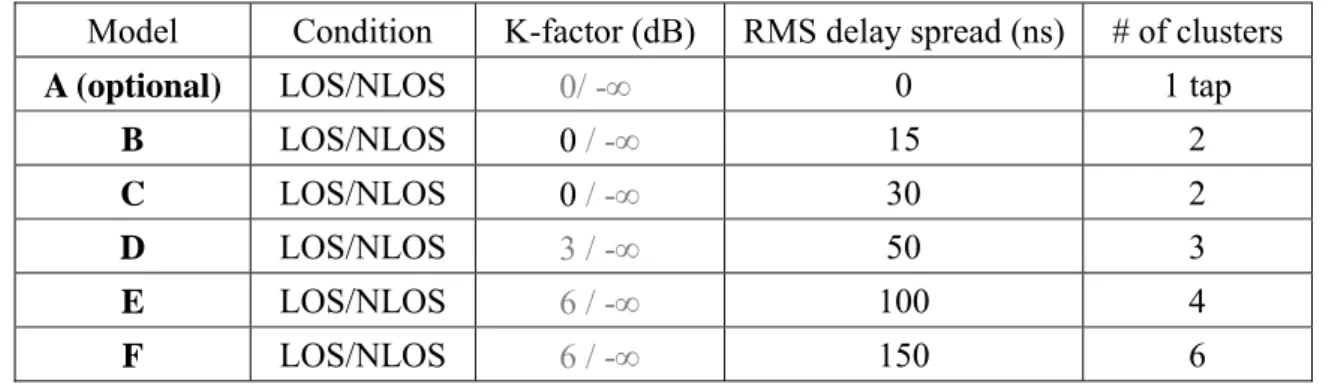
Properties of these models are shown in Table 2-2 and Table 2-3.Here, K-factor for the LOS

condition applies only to the first tap, and K- factor= −∞(dB) applies to all other taps. There is

another factor d_BP called the breakpoint distance. If the transmit-receive separation distance is

set less thand_BP, the channel will be considered as the LOS condition. If the transmit-receive

separation distance is greater thand_BP, the channel will be considered as the NLOS condition.

Model Condition K-factor (dB) RMS delay spread (ns) # of clusters

A (optional) LOS/NLOS 0/ -∞ 0 1 tap

B LOS/NLOS 0 / -∞ 15 2

C LOS/NLOS 0 / -∞ 30 2

D LOS/NLOS 3 / -∞ 50 3

E LOS/NLOS 6 / -∞ 100 4

F LOS/NLOS 6 / -∞ 150 6

Table 2-2: Model parameters for LOS/NLOS conditions

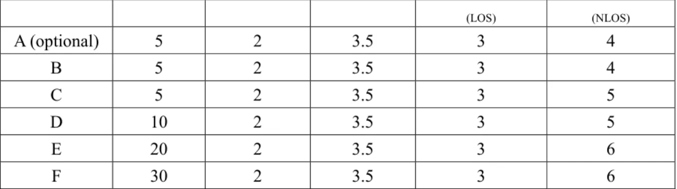
New Model dBP (m) Slope before

dBP Slope after dBP Shadow fading std. dev. (dB) before dBP Shadow fading std. dev. (dB) after dBP

(18)

(LOS) (NLOS) A (optional) 5 2 3.5 3 4 B 5 2 3.5 3 4 C 5 2 3.5 3 5 D 10 2 3.5 3 5 E 20 2 3.5 3 6 F 30 2 3.5 3 6

Table 2-3: Path loss model parameters

We choose the channel-B (NLOS) with distance 6m, channel-D (NLOS) with distance 11m, and channel-E (NLOS) with distance 21m as our simulation environments in this thesis. Besides, the time resolution of the channel model is 10ns, which is one-fifth of the sampling period (3.2ms/64=50ns). We oversample the transmitted signal by a factor of 5 and interpolate it linearly in order to convolve with the response generated by the channel model.

2.3 System Model

Before our formal development, we define notations will be used in the sequel. Scalars are denoted in lower case letters, vectors in lower case italic letters, and metrics in upper case bold

letters. Also,

[ ]

.T

and

[ ]

. H

indicate the transpose and conjugate transpose of a vector or matrix inside the bracket respectively. Since 802.11n is designed to be used in the indoor environment, we can assume that the MIMO channel is a multi-path quasi-static Rayleigh fading channel. The

frequency response of the MIMO channel at the th

k sub-channel is defined as 1,1 1, , ,1 , T R R T k k N k k q p k k N N N h h h h h ⎡ ⎤ ⎢ ⎥ = ⎢ ⎥ ⎢ ⎥ ⎣ ⎦ H (2.1)

where p represents the index of the transmit antenna, q the index of the receive antenna, T

N the number of transmit antennas, and N the number of receive antennas. The transmitted _R

symbol vector at the th

(19)

, , , 1 s , , T T l k l k l k N s s ⎡ ⎤ = ⎣ ⎦ (2.2)

The received symbol vector at the th

k sub-channel and the l OFDM symbol after th

GI-Remover/FFT is defined as , , , 1 , , R T l k l k l k N r r ⎡ ⎤ = ⎣ ⎦ r (2.3)

Assume that there are no inter symbol interference (ISI) and inter carrier interference (ICI).

Then, l k, r can be represented as , _s, , l k = k⋅ l k + l k r H n (2.4) where , , , 1 , , R T l k l k l k N n n ⎡ ⎤ = ⎣ ⎦ n (2.5)

is the received noise vector, and each element in n_{l k}_, is statistically independent and

identically distributed (i.i.d.) complex Gaussian random variable with zero mean and

variance 2 2 2

0

I Q N

σ =σ +σ = . Signal to noise ration (SNR) is defined as the average received

power per receive antenna divided by the average noise power.

( )

{ }

2 2 q E r t SNR σ ′ = (2.6)

where r t_q′

( )

represents the received signal at time t at the q transmit antenna. For th

simplicity, we ignore the index k and l in the rest of this thesis. Then, we have s

= ⋅ +

r H n (2.7)

2.4 Bit-Interleaved Coded Modulation

First of all, we would review two existing demodulation schemes on BICM structure. The first one “decouples” the MIMO symbol vector to single-input-single-output (SISO) scalar

(20)

signals by a ZF/MMSE equalizer. And then it calculates the soft coded bits information with a SISO soft-demapper, and feed the result to the FEC decoder. The scheme is simple and the required computational complexity is low, but it is not optimal. In many cases, its performance becomes not acceptable. The other one calculates the soft “coded bits” information using a MIMO soft-demapper directly. This is an optimum approach; however, its computational complexity can be very large and it is not feasible in real-world systems in general. In [10], a low-complexity algorithm overcoming the problem, named LSD, was proposed. Note that to apply the “iterative decoding” technique, we have to use the MIMO soft-demapper. This is because soft-bit information calculated with the equalization-and-SISO-soft-demapping approach is not accurate enough. As a result, the error will be propagated during iteration, yielding poor performance. The iterative decoding (Turbo equalization) proposed by [5] exchanging the coded bits extrinsic information between the equalizer and the channel decoder. As will be shown later, turbo equalization can greatly enhance the performance of MIMO-OFDM systems.

2.5 Suboptimal Receiver with the MMSE Equalizer

Here, let the FEC coder be the CC coder. Since the performance of the MMSE equalizer is better than the ZF equalizer, we only consider the MMSE equalizer. This receiver scheme includes a MMSE equalizer, a SISO soft-demapper, and an optimum decoder, called the BCJR decoder [7]. First, the received symbol vector is processed by the MMSE equalizer, which decouples the MIMO symbol vector to multiple SISO signals. For each SISO signal, we apply a SISO soft-demapper to obtain soft coded bit information. Finally, the whole soft-bit stream is fed into the BCJR decoder to detect information bits. The block diagram of the MIMO-OFDM transceiver is shown in Fig. 2-2 and Fig. 2-3.

(21)

Fig. 2-2: The block diagram of the MIMO-OFDM transmitter for BICM soft-input BCJR decoder de-puncture de-parser de-interleaver soft-bit de-mapper GI remover /FFT

de-interleaver de-mappersoft-bit GI remover/FFT MMSE equalizer ( ) ( )

{

, , , , , , ,

}

p p l k I m l k Q m c c ∧ ∧ analog/RF analog/RF , l k p y l k, q r r t_q′( ) Fig. 2-3: The block diagram of the MIMO-OFDM receiver for BICM

2.5.1 Minimum Mean-Square Error (MMSE) Equalizer

Assume that the received symbol vector： =r H s n⋅ + . We define an error vectore , which is _k

the error between the received signal and the MMSE equalizer output y . That is

2 2

arg min{ } arg min{ }

MMSE MMSE

H

MMSE MMSE

G G

G = y s− = G r s− (2.8)

With the Wiener-Hopf equation, we can have

1 * [ ] r r H MMSE N N G = HH +αI − H (2.9) where 2 2 noise per antenna σ α σ − = , 2 noise

σ is the additive complex Gaussian noise variance, 2

per antenna

σ ₋ is

the average transmission power over per antenna. Finally, the MMSE equalizer output can be obtained as 1 [ ] T T H k = y ⋅⋅⋅yN =GMMSE⋅ k y r (2.10)

(22)

2.5.2 Simplified Soft-Bit Demapper for SISO-OFDM system

After equalization, the MIMO signal is decoupled into SISO signals. We can then use SISO soft-demappers [8] calculate coded bits information. Let M be the size of castellation in

Gray-mapping, where N_bpsc =log ( )₂ M is the number of coded bits in one QAM symbol. That is,

2 bpsc

N coded bits are mapping to the in-phase or quardrature-phase part of QAM symbol. Soft

bit information is generally represented by LLR, defined as

(1) , ( 0) , , , , ( ) ( 1 ) ( ) log( ) log( ) ( 0 ) ( ) j I i j I i j s I i I i I i j s p s r p c r LLR c p c r p s r ∈ ∈ = = =

∑

s s (2.11) where the (1) , I i

s comprises the set of symbols on certain transmitter antenna with a ‘0’ in

position (I, i).

The LLR can be simplified by using the log-sum approximation as:

log( _j) max{log( )}_j

j

p ≈ p

∑

(2.12)

The approximation error will be small if the terms in the left-hand side of (2.13) is dominated by the largest one. This is true when SNR is high. Then, we have

(1) , (1) (0) , , ( 0) , max{ ( )}

log( ) log max{ ( )} log max{ ( )}

max{ ( )} j I i j I i j I i j I i j s j j s s j s p s r p s r p s r p s r ∈ ∈ ∈ ∈ = − s s s s (2.14)

The SISO system can be modeled as r h s n= ⋅ + (we omit the index p and the index q

for simplicity). Since N =1 and _T N =1, and R

2 2 2 1 1 ( ) exp 2 j j r h s p s r πσ σ ⎧ _{− ⋅} ⎫ ⎪ ⎪ = _⎨− _⎬ ⎪ ⎪ ⎩ ⎭ , we can rewrite (2.14) as

(23)

(1) (0 ) , , (0) (1) , , 2 2 , 2 2 2 2 2 2 , 2 1 ( ) min{ } min{ } = min{ } min{ } = j I i j I i j I i j I i I i j j s s j j s s I i LLR c r h s r h s h y s y s h D σ σ σ ∈ ∈ ∈ ∈ ⎧ ⎫ = _⎨− − ⋅ + − ⋅ _⎬ ⎩ ⎭ ⎧ ₋ ₋ ₋ ⎫ ⎨ ⎬ ⎩ ⎭ s s s s (2.15) where [ ₁ ] T T k = y ⋅⋅⋅yN

y is the equalizer output. From (2.15), we can see that only the

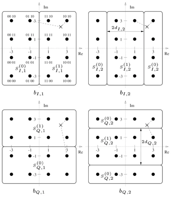
distance between the two nearest QAM symbol on set 0 or 1 is required to calculate the LLR. Note that for the Gray mapping scheme, some simple rules exist such that the distance can be found with a low computational complexity. It turns out that we only have to partition the constellation plane, horizontally or vertically (corresponding to in-phase or quardrature-phase part), and find the nearest QAM mapping points of the two set, which are always laid on a same vertical or horizontal or straight line. The observation holds for 16 and 64-QAM constellation. For 16 QAM constellations, we can derive the distance in the in-phase part as [8]

,1 ,2 , 2 2( 1) 2 2( 1) 2 2 I I I I I I I I I y y D y y y y D y ⎧ ≤ ⎪ =_⎨ − > ⎪ ₊ _{< −} ⎩ = − + (2.16)

It can be easily verified that D_{Q i}_, for the two quadrature bits are the same as that calculated

in (2.16) with y replaced by _{I i}_, y_{Q i}_, .

The block diagram of the SISO-OFDM transceiver (for BICM) is shown in Fig. 2-4 and Fig. 2-5

(24)

FEC encoder puncture bit-level interleaver QAM mapper IFFT/GI , l k s analog/RF

Fig. 2-4: The block diagram of the SISO-OFDM transmitter for BICM

soft-input Viterbi decoder de-puncture de-interleaver soft-bit de-mapper GI remover /FFT , l k r , l k y analog/RF MMSE equalizer ( ) q r′ t

Fig. 2-5: The block diagram of the SISO-OFDM receiver using the MMSE equalizer for BICM

(25)

2.6 Optimal Receiver with LSD

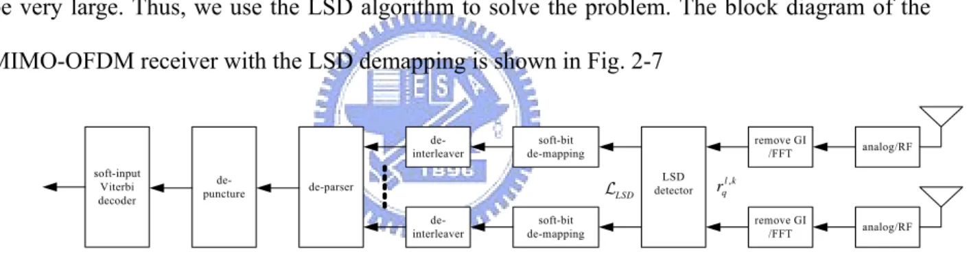
In the previous section, we can see that the MIMO symbol vector can be decoupled by a MMSE equalizer, and coded bit information can be obtained by SISO soft demappers. The receiver structure is simple and the required computational complexity is low. However, the noise after equalization becomes colored. Also, signals from different antennas may become correlated. The optimality of the BCJR decoder is based on the assumption that the noise is white and the signals are independent to each other. Thus, the conventional approach is not optimal. To solve this problem, we use a MIMO soft-demapper,, instead of an equalizer and SISO soft-demappers. It has been known that the computational complexity of the optimum MIMO soft-demapping can be very large. Thus, we use the LSD algorithm to solve the problem. The block diagram of the MIMO-OFDM receiver with the LSD demapping is shown in Fig. 2-7

soft-input Viterbi decoder de-puncture de-parser de-interleaver soft-bit de-mapping remove GI /FFT de-interleaver soft-bit de-mapping remove GI /FFT LSD detector analog/RF analog/RF LSD L l k, q r

Fig. 2-7: The block diagram of the MIMO-OFDM receiver using the LSD detector for BICM

2.6.1 Optimum MIMO Soft-Demapping

The received symbol vector of a MIMO-OFDM system can be modeled as:

1 = s , [ ] T T N r r ⋅ + = ⋅⋅⋅ r H n r (2.17)

If we use 2M_{-QAM transmission, and the number of transmit antenna is}

T

N , there will be a

total of M N⋅ _T bits in the received symbol vector r . With the MIMO soft-demapping, we

calculate the coded bit LLR directly without equalization. Now, we find the nearest symbol vectors belonging to two sets (0 or 1) based on the received symbol vector, instead of an

(26)

individual scalar signal. That is: (1) , (0) , φ , , , φ (φ ) Pr[ 1 ] ( ) log( ) log( ) Pr[ 0 ] (φ ) j k i j k i j k i k i k i j p c LLR c c p ∈ ∈ = = =

∑

s s r r r r (2.18)

where c is the i-th bit on k-th transmitter antenna, _{k i}_, s(1)_{k j}_, is the set of symbol vectors with

‘0’ on position (k, i). φ [ , ,₁ ]

T

j = ϕ … ϕN is the possible symbol vector belonging to

(1) ,

k j s .

According to Baye’s rule, we can derive the probability density function of (φp _j r as: )

( φ ) (φ ) (φ , ) (φ ) ( ) ( ) j j j j p p p p p p ⋅ = r = r r r r (2.19)

Assuming that the appearing probability of each symbol (φ )p j , is equally probable. So,

(φ )_j

p and ( )p r can be canceled in the LLR calculation. We then have

( )

2 2 2 1 1 ( | φ ) exp φ 2 r j N j p σ πσ ⎧ ⎫ = _⎨− − ⋅ _⎬ ⎩ ⎭ r r H (2.20)

Equation (2.18) can now be rewritten as:

(1) , ( 0) , (1) (0) , , (0) (1) , , φ , φ φ φ 2 2 2 _φ _φ (φ ) ( ) log( ) (φ )

log max( ( φ )) log max ( ( φ )) 1 min { φ } min{ φ } 2 j k i j k i j k i j k i j k i j k i j k i j j j j j p LLR c p p p σ ∈ ∈ ∈ ∈ ∈ ∈ = ≈ − ⎧ ⎫ ≈ _⎨ − ⋅ − − ⋅ _⎬ ⎩ ⎭

∑

s s s s s s r r r r r H r H (2.21)

Though the max-log theorem simplifies the calculation, the required computational complexity is still very large when the number of transmit antennas and the QAM size become

large. For example, when the number of transmitter antenna is 4 (N =4) and the modulation is _T

(27)

be tested. In order to reduce the complexity, we use the LSD algorithm.

2.6.2 List Sphere Decoding (LSD)

A simply way to approximate (2.21) is to consider only the symbol vectors whose distance

2

φ − ⋅

r H is small. As a result, we can have a “list” of candidate symbol vectors, and find the

minimum in the list instead of the exhausted search. Searching the list generally provides a good approximation of (2.21), if the distance is carefully chosen. Observe that:

(

)

(

)

(

)

1

)

2

φ φ H _H φ _H _H − _H

− ⋅ = − ⋅ ⋅ ⋅ − + ⋅ − ⋅ ⋅ ⋅ ⋅

r H y H H y r I H H H H r (2.22)

where y is the equalizer output in (2.10). The LSD algorithm find those symbol vectors

with distance small than r_LSD, where is:

(

)

(

)

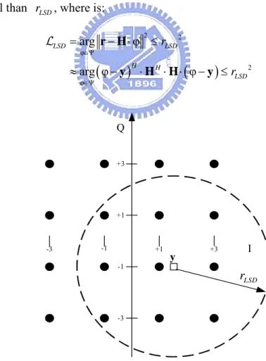
2 2 φ 2 φ arg φ arg φ φ LSD LSD H _H LSD r r ∈Ψ ∈Ψ = − ⋅ ≤ ≈ − ⋅ ⋅ ⋅ − ≤ r H y H H y L (2.23) +3 +1 -3 -1 +3 +1 -1 -3 Q I y LSD r

(28)

where

T

1

[ψ ψ_N ]

Ψ = ⋅⋅⋅ represents the subset of all possible symbol vectors from the

constellation map. The LSD detector only checks those symbol vectors lying inside a sphere as shown in Fig. 2-8.

We now show how to implement the idea. Applying Cholesky factorization, we factorize H as upper triangular U H _{⋅ =} H_⋅ U U H H (2.24) where 1,1 1, , , ... T T T N i i N N u u u o u ⎡ ⎤ ⎢ ⎥ = ⎢ ⎥ ⎢ ⎥ ⎣ ⎦ U (2.25)

It can be proved that U is positive and real. Then, (2.23) can be modified as

(

)

(

)

2 φ 2 2 2 2 2 , , 1 1 arg φ φ T T H H LSD N N i i i i i j j j LSD i j i r u ϕ y u ϕ y r ∈Ψ = = + − ⋅ ⋅ ⋅ − ≤ ⎛ ⎞ ⇒ _⎜ − + − _⎟≤ ⎝ ⎠

∑

y U U y (2.26)

With the transformation, we can search the candidates in a tree structure. We start from T

i=N and accumulate the distance, layer by layer. If the distance of one branch is smaller than

2

LSD

r , we continue to calculate the branch distance extending from this branch. If the distance is

larger than 2

LSD

r , we prune this branch.

After obtaining the list L_LSD , we can find the one with the minimum distance in the sets

with the indicated bit is ‘0’ and ‘1’ . We can rewrite (2.21) to:

(0) (1) , , (0) (1) , , 2 2 , 2 _φ _φ 2 2 2 _φ _φ 1 ( ) min { φ } min{ φ } 2 1 min { φ } min { φ } 2 j k i j k i j k i LSD j k i LSD k i j j j j LLR c σ σ ∈ ∈ ∈ ∩ ∈ ∩ ⎧ ⎫ ≈ _⎨ − ⋅ − − ⋅ _⎬ ⎩ ⎭ ⎧ ⎫ ≈ _⎨ − ⋅ − − ⋅ _⎬ ⎩ ⎭ s s s s r H r H r H r H L L (2.27)

(29)

2.6.3 Real-Valued LSD

In the QAM transmission, the real and the imaginary parts of the received symbol vector r can be considered to be independent. The channel matrix H and the symbol vector s can also be decomposed into real and imaginary parts. That is, we can transform the original

complex-valued LSD to the real-valued LSD with 2⋅N_T dimensions. Then, (2.26) can be

revised to

(

)

(

)

(

)

(

)

2 φ 2 φ arg φ φ arg φ ' ' ' ' φ ' ' H _H LSD H H LSD r r ∈Ψ ∈Ψ − ⋅ ⋅ ⋅ − ≤ ⇒ − ⋅ ⋅ ⋅ − ≤ y U U y y U U y (2.28) where

{ } { }

{ }

' Re Im φ ' Re φ Im φ Re Im ' Im Re T T T T T T ⎡ ⎤ = ⎣ ⎦ ⎡ ⎤ = ⎣ ⎦ − ⎡ ⎤ = ⎢ ⎥ ⎣ ⎦ y y y U U U U U (2.29)

With this approach, the computational complexity of the LSD can be further reduced since more symbol vectors will be pruned in early stages. However, the latency of the real-valued LSD becomes larger due to the higher dimensions.

2.6.4 Radius of the Sphere

The size of the list L_LSD determines how well (2.27) can approximate (2.21). If the radius is

too small, no symbol vectors will be found. If the radius is too large, the number of symbol vectors in the list will be too large, and the complexity will be high (though it can approach the optimum solution better). How to determine the radius becomes a critical problem. In [5], a

(30)

simple method for the determination of the radius is proposed. Assuming that the true transmitter

symbol vector is s_true, we then have

2 2 ₂ ₂ s T true σ χN − ⋅ = ⋅ r H n ∼ (2.30) where 2 T N

χ is a random variable having a chi-square distribution with N degrees of _T

freedom. However, note that the vector used for distance calculation is transformed by the matrix

U. The distribution of the squared-distance will be highly depended on H , In [16], the radius is

given by

1/

2 _{det( )} NR

LSD LSD

r =C ⋅ H (2.31)

where C_LSD is a real constant greater than 1. Once a suitable CLSD is chosen, we can

determine the radius of LSD. We will use the method in our later development. However, even

for a good C_LSD, there will be no guarantee that at least one candidate will be in the sphere. If no

candidates are found, the radius needs to be enlarged and repeat the search until L_LSD ≠ ∅. In

case of that one of the two sets ( (1)

,

k i

s and s(0)k i, ) is empty, we can simply assign the LLR as an

extreme value representing that the probability of the bit being 1 or 0 is high.

2.7 Turbo Equalization

With the optimum MIMO soft-demapping, we have greatly enhanced the performance of the MIMO-OFDM receiver. However, demapping and decoding are still conducted separately. In other words, the true optimum performance for the receiver is not achieved. To solve the problem, demapping and decoding should be considered jointly. However, this will results in a prohibited computational complexity. Turbo equalization, an iterative detection method, can effectively solve the problem. We can treat the MIMO channel as an inner encoder, and the CC as an outer encoder. Since an interleaver has been equipped between these two encoders, the combination of

(31)

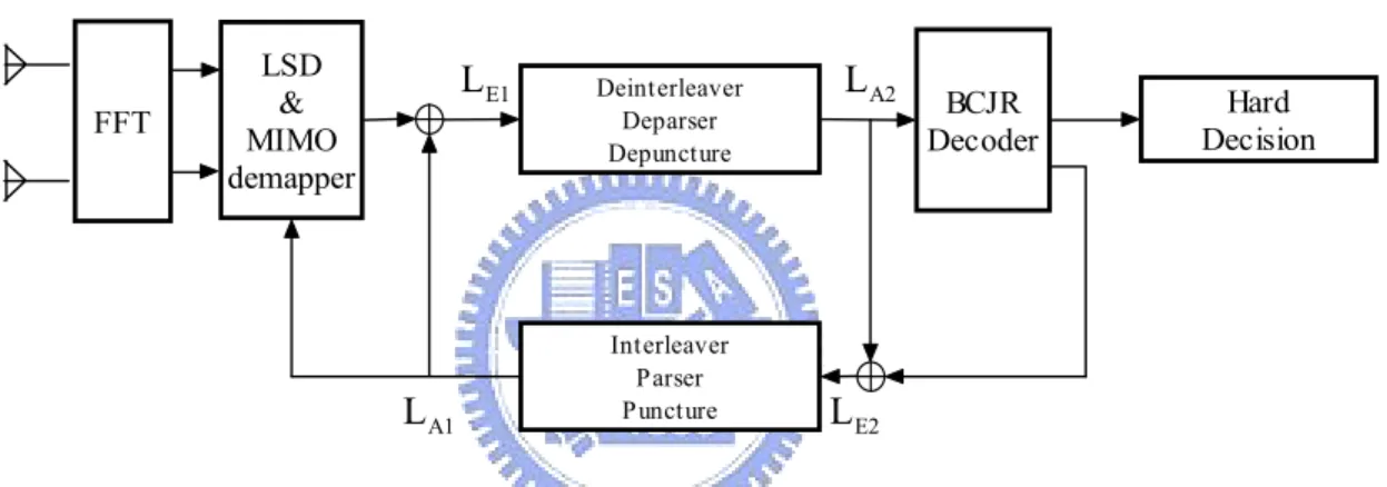
these devices resembles a turbo code structure. The iterative process can be described as follows. The outer decoder processes the soft information from the demapper, and generates its own soft information indicating the relative likelihood of each of the coded bits. This soft information from the outer decoder is then fed back to the demapper, creating a feedback loop between the demapper and decoder. The operation is repeated until a stopping criterion is met. This process is often termed “belief propagation” or “message passing” and has a number of important connections to methods in artificial intelligence, statistical inference, and graphical learning theory. Fig. 2-9 gives a flowchart of turbo algorithm that we use.

FFT LSD & MIMO demapper Deinterleaver Deparser Depuncture BCJR Decoder Interleaver Parser Puncture Hard Decision A2 L A1 L E1 L E2 L

Fig. 2-9: Diagram of turbo processing for the OFDM-MIMO system

The LSD and the MIMO demapper takes observations and a priori coded bits information

1

A

L to compute new (also referred to as “extrinsic”) coded bits information

1

E

L for each of the

received symbol vector. Then

1

E

L is de-interleaved and rearranged to become the a priori input

2

A

L to the outer soft-in/soft-out maximum a posteriori probability (MAP) decoder, which

calculates extrinsic coded bits information

2

E

L and the information bits LLR. Then L is E₂ re-interleaved and feedback as a priori information to the MIMO soft-demapper. This completes one iteration. Each iteration can reduce the bit-error rate by exchanging information between the inner and the outer decoder.

(32)

2.7.1 BCJR Algorithm on Convolutional code decoder

In order to minimize the probability of error for each detected symbol and calculate the soft coded bits information, we use the MAP detector instead the Viterbi decoder [9]. The algorithm for the MAP detection is termed the BCJR algorithm [7] in the literature. The original BCJR algorithm was expressed in the probabilistic form. For example, to make a decision about the

information bit of k-th stage b , this decoder calculates the a posteriori probability _k Pr[b r for _k ]

each possible b_k∈{0,1}, and decides on the b that maximizes k Pr[b r . In the convolutional k ]

code trellis diagram, these probabilities are easily computed once the a posteriori state transition

probability Pr[Ψ =_k p; ]Ψ_k+₁= c is known for each state transition in the trellis. The BCJR q

(Bahl, Cocke, Jelinek and Raviv) algorithm [7] provides a computationally efficient method for finding these state transition probabilities.

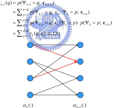
The key to the BCJR algorithm is to decompose a posteriori state transition probability into three separable parts, and use a recursive technique to calculate the transition probability. We start from the a posteriori probability in convolutional trellis structure.

1 ( , ) Pr[ ] Pr[ ; ] a k k k p q S b p ₊ q ∈ =

∑

Ψ = Ψ = c c (2.32)

where p q, ∈ …

{

1 Q

}

is the state of convolutional code, the c is the coded bits probability. We

can calculate the a posteriori transition probability of certain information bit by summarizing a

set of transition probabilities S whose certain information bit is 0 or 1. _a

We now can further decompose the transition probabilities of such stage into three parts: the

first c_{l k}< =

{

c :_l l<k

}

only depends on the “past” observations, the second one only depends on

(33)

{

c :

}

l k> = l l>k

c . We can accomplish this through the following series of equalities.

1 1 1 1 1 Pr ; ( ; ; ) ( ) ( ; ; ; c ; ) ( ) ( ; ; ; c ) ( ; ; ; c ) ( ) k k k k k k l k k l k l k k k l k k k k l k k p q p p q p p p q p p p q p p q p + + + < > > + < + < ⎡Ψ = Ψ = ⎤= Ψ = Ψ = ⎣ ⎦ = Ψ = Ψ = = Ψ = Ψ = ⋅ Ψ = Ψ = c c c c c c c c c c (2.33) Due to the Markov property of the finite-state machine model for the channel, knowledge of the sate as time k+1 supersedes the knowledge of the state at time k, and it also supersedes

knowledge of c_{l k}_< and ck, so (2.33) can be reduced to

1 1 1 1 1 Pr ; ( ) ( ; ; ; c ) ( ) ( ) ( ; c ; ) ( ; ) ( ) k k l k k k k l k k l k k k k k l k k l k p q p q p p q p p q p q p p p p + > + + < > + + < < ⎡Ψ = Ψ = ⎤= Ψ = ⋅ Ψ = Ψ = ⎣ ⎦ = Ψ = ⋅ Ψ = Ψ = ⋅ Ψ = c c c c c c c c (2.34) Again, exploiting the Markov property, we can simplify (2.34) to:

1 1 1 1 ( ) ( , ) ( ) Pr ; ( ; ) ( ; c ) ( ) ( ) k k k k k k l k k k k l k k p p q q p q p p p q p p q p α γ β+ + < + > + ⎡Ψ = Ψ = ⎤= Ψ = ⋅ Ψ = Ψ = ⋅ Ψ = ⎣ c⎦ c c c (2.35)

Observe that α_k( )p is the probability measure for state p at stage k that depends only on the

past observationsc_{l k}_< . βk+1( )q , on the other hand, is a probability measure for state q at stage

k+1 that depends only on the future observationsc_{l k}_> . And γk( , )p q is a probability measure connecting state p at stage k and the state q at stage k+1, and also, it depends only on the present

observation c_k.

Now we can derive (2.32) by using (2.35)

1 ( , ) 1 ( , ) Pr[ ] Pr[ ; ] 1 ( ) ( , ) ( ) ( ) a a k k k p q S k k k p q S b p q p p q q p α γ β + ∈ + ∈ = Ψ = Ψ = = ⋅ ⋅

∑

c c c (2.36)

(34)

following. We start from the “present” branch metric γ_k( , )p q . According to (2.35) 1 1 1 ( , ) ( ; r ) (c ; ) Pr[ ] k k k k k k k k k p q p q p p p q q p γ ₊ + + = Ψ = Ψ = = Ψ = Ψ = ⋅ Ψ = Ψ = (2.37)

where the first part is the product of certain coded bits probability, according to the transition codeword.

(

1

)

1 c ; ( ) n k k k i j p p ₊ q p c = Ψ = Ψ = =

∏

(2.38)

And the second part of the equality is the priori information of transition codeword. Generally we assume all input sequences with equal probability, so the priori probability of each codeword is a

const. We now derive a recursive technique for calculating αand β

1 1 1 1 1 1 1 1 ( ) ( ; ) ( ; c ; ; ) ( ; c ) ( ; ) ( , ) ( ) k k l k p Q k k k l k p p Q k k k k l k p p Q k k p q p q p q p p q p p p p q p α γ α + + < + = + < = = + < = = = = Ψ = = Ψ = Ψ = = Ψ = Ψ = ⋅ Ψ = = ⋅

∑

c c c (2.39) (:) k α αk+1(:)

Fig. 2-10: Recursive calculating of α in trellis diagram

(35)

1 1 1 1 1 1 1 1 1 1 ( ) (c ) (c ; c ; ) (c ) (c ; ) ( ) ( , ) k l k k p Q l k k k k p p Q l k k k k k p p Q k k p p p p p q p p q p q p q p q β β γ > − = > − + = = > − + + = = + = = Ψ = = Ψ = Ψ = = Ψ = ⋅ Ψ = Ψ = = ⋅

∑

(2.40) (:) k β βk+1(:)

Fig. 2-11: Recursive calculating of β in trellis diagram

We now make two passes, α forward pass from beginning to the end and β backward

pass from finish to start. After we calculate all state probabilities in the trellis, we can calculate the information bits LLR by

(1) ( 0) 1 ( , ) 1 ( , ) Pr( 1 ) ( ) log( ) Pr( 0 ) ( ) ( , ) ( ) log( ) ( ) ( , ) ( ) k k k k k k k k p q B k k k p q B b LLR b b p p q q p p q q α γ β α γ β + ∈ + ∈ = = = ⋅ ⋅ = ⋅ ⋅

∑

c c (2.41)

(36)

(1) , (0) , (1) , 2 , , , 1 ( , ) 1 ( , ) 1 ( , ) , , ( , ) Pr( 1 ) ( ) log( ) Pr( 0 ) ( ) ( , ) ( ) log( ) ( ) ( , ) ( ) ( ) ( , ) ( ) ( 1) log( ) log( ( 0) ( ) k i k i k i A k i k i k i k k k p q C k k k p q C k k k p q C k i k i k p q C L c LLR c c p p q q p p q q p p q q p c p c p α γ β α γ β α γ β α + ∈ + ∈ + ∈ ∈ = = = ⋅ ⋅ = ⋅ ⋅ ⋅ ⋅ = = + =

∑

c c ( 0) , 2 , 1 ) ( ) ( , ) ( ) k i E k i k k L LLR c p q q γ β + − ⋅ ⋅

∑

(2.42)

2.7.2 List Sphere Decoding with Priori Information

With the coded bits priori information calculated by the outer BCJR decoder, we can modify the original LSD to have another form. Meanwhile, we assume that we are working on a block of

bits corresponding to one symbol vector φ_j. The a posteriori LLR of the coded bit on certain

antenna, conditioned on the received symbol vector r , is:

, , , ( 1 ) ( ) log( ) ( 0 ) i k i k i k p c LLR c p c = = r r (2.43)

We now assume the bits on φj have been encoded with channel, and the interleaver is used

to scramble the bits from other antennas. So, the bits within φ_j are approximately statistically

independent of one another. Using the Bayes’ theorem, and splitting the joint probability, we can have the soft output value as

(1) , ( 0) , , , φ , , , φ ( ) ( φ ) exp ( ) ( ) ( ) log( ) ( φ ) exp ( ) k j k i k j k i E k i j A k i l D k i A k i j A k i l L b p L c L c L c p L c ∈Ω ∈ ∈Ω ∈ ⋅ = + ⋅

∑

s s r r (2.44) where (1) , k j

(37)

,

k i

b =1. Ω is the set of indices l with _k

{

0, , 1, ( , )

}

k l l NT M l k i Ω = = … ⋅ − ≠ (2.45) , , , ( 1) ( ) log( ) ( 0) k i A k i k i P c L c P c = = = (2.46)

Multiplying the numerator and the denominator with

1 1 , 0 exp( 1 2 NTM ( )) A k i l L c ⋅ − = − ⋅

∑

, we can rewrite (2.44) as (1) , 1 ( 0 ) , , 1 , [ ] ,[ ] φ , [ ] ,[ ] φ ( ) ( ) 1 ( φ ) exp 2 = ( ) log( ) 1 ( φ ) exp 2 j k i j k i E i k D k i T j j A j A k i T j j A j L c L c p L c p ∈ ∈ ⎛ ⎞ ⋅ _⎜ ⋅ _⎟ ⎝ ⎠ + ⎛ ⎞ ⋅ _⎜ ⋅ _⎟ ⎝ ⎠

∑

s s r b L r b L (2.47)

where b_{[ ]}_j denotes the vector which omitting its j-th element, which is the position of c . _{k i}_,

1 2 (1) , (0) , [ ] 1 if φ 1 if φ T N M j k i i j k i b b b b ⋅ = ⎧ ∈ ⎪ = ⎨₋ _∈ ⎪⎩ b s s … (2.48)

and L_{A j}_{,[ ]} denote s the vector form of all L except the same term. Further, we can use the A

max-log approximation to simplify(2.47) , that is

( 0) 1 , (1) , 1 2 , , _{2 φ} [ ] ,[ ] 2 [ ] ,[ ] 2 φ 1 1 ( ) ( ) min { φ } 2 1 1 min{ φ } 2 j k i j k i E T i j A k i j j A j T j j A j L LLR c L c σ σ ∈ ∈ ⎧ ⎫ ≈ + _⎨ − ⋅ + ⋅ _⎬ ⎩ ⎭ ⎧ ⎫ − _⎨ − ⋅ + ⋅ _⎬ ⎩ ⎭ s s r H b L r H b L (2.49)

2.7.3 MIMO Detection Using the List Sphere Decoder

As mentioned, we use the LSD to help find the candidates that can be used to compute soft bit

(38)

the candidates in L_LSD as (0) 2 , (1) , 2 2 , , _{2 φ} [ ] ,[ ] 2 [ ] ,[ ] 2 φ 1 1 ( ) ( ) min { φ } 2 1 1 min { φ } 2 j LSD k i j LSD k i E T i j A k i j k A k T j k A k L LLR c L c σ σ ∈ ∩ ∈ ∩ ⎧ ⎫ ≈ + _⎨ − ⋅ + ⋅ _⎬ ⎩ ⎭ ⎧ ⎫ − _⎨ − ⋅ + ⋅ _⎬ ⎩ ⎭ s s r H b L r H b L L L (2.50)

There is also tradeoff between the accuracy of (2.50) and the computational complexity of the LSD. When the size of the list is too small, the soft bit information is not accurate enough such

that the “turbo” scheme may not work. The reason is that L_LSD may not contain the true

transmitter symbol vector, the coded bits LLR generated by the outer coder will not contain the soft information of the true transmitter symbol vector. As a result, the LLR will not be increased toward the right direction. On the other hand, if the size of the list is too large, the computational complexity of the LSD will become too high, adversely affecting the applicability of the turbo equalization scheme in real-world systems.

2.8 Simulation Results

Our simulation platform is developed based on the IEEE802.11n proposal. We use the mandatory mode in which the constraint length of the convolutional code is 7, the channelization bandwidth is 20MHz (56 occupied sub-channels), and the number of spatial streams is two

T

N =2 and N =4. The number of receive antennas is the same as that of transmit antennas. Two T different systems with the same throughput are considered.

(a) Conventional equalization and SISO demapping: An MMSE equalizer, a SISO

soft-bit demapper, and a BCJR decoder are used at the receiver. In the figures shown later, we use “SB” to denote this approach.

(b) Turbo Equalization: A LSD detector, MIMO soft-demapper, a BCJR decoder, and

(39)

“TE” in the figures shown below. The dash “TE” indicates the iteration number. Assume that the frequency offset and timing offset are perfectly compensated at the receiver. We use the HT-LTF of the preamble and the standard per-tone channel estimation method (no smoothing) to estimate MIMO channels. The PPDU length is set as 1000 bytes; so there are 8000 information bits in each packet. The packet error rate (PER) is used as the performance measure. We choose the channel-B (non-line-of -sight) [15], and the channel-D (non-line-of -sight) as simulation environments. Fig. 2-12 to Fig. 2-17 show the simulation results for the perfect-channel cases. Fig. 2-18 to Fig. 2-23 show the results for the estimated-channel cases. For all case, the turbo scheme performs much better than the conventional schemes. From Fig. 2-12 to Fig. 2-17, we observe that when PER is 0.1 and channel-B is considered, the turbo scheme with zero iteration outperforms the conventional scheme about 3dB in 2X2 16-QAM, 10dB in the 4X4 16-QAM, 12dB in 4X4 64-QAM scenarios. With iterations, the performance is further improved. The performance improves about additional 2dB with one iteration, and further 0.5dB with four iteration. In channel-D environment, the improvement of the turbo scheme with zero iteration is less than channel-B. But it still has 3dB, 7dB, and 9dB gain in the 2X2 16-QAM, 4X4 16-QAM, and 4X4 64-QAM scenarios. From Fig. 2-15 to Fig. 2-17, we can see that the gain due to iterations is almost the same as channel-B. From the result, we can conclude that the MIMO soft-demapping is the major factor for performance improvement. From implementation point of view, we can see that the turbo scheme only requires one iteration.

(40)

Fig. 2-12: Performance comparison of soft+BCJR and Turbo scheme (20MHz, 2x2, 16-QAM, channel-B, perfect-channel)

:

(41)

Fig. 2-15: Performance comparison of soft+BCJR and Turbo scheme (20MHz, 2x2, 16-QAM, channel-D, perfect-channel)

(42)

(43)

From Fig. 2-18 to Fig. 2-23 show the simulation results for estimated channels. The standard per-tone channel estimation method (no smoothing) is used to estimate the MIMO channel. In channel-B, the improvement of the turbo scheme with zero iteration is 4dB, 10dB, and 11dB in the 2X2 16-QAM, 4X4 16-QAM and 4X4 64-QAM scenarios, respectively. The gain, due to iterations, is about 2 dB with one iteration, and additional 0.5dB with four iterations. In

channel-D, the improvement with zero iteration is 3dB, 6dB, and 8dB in the 2X2 16-QAM, 4X4 16-QAM and 4X4 64-QAM scenarios, respectively. The gain due to iterations is similar to that in channel-B.

Fig. 2-18: Performance comparison of soft+BCJR and Turbo scheme (20MHz, 2x2, 16-QAM, channel-B, estimated-channel)

(44)

(45)

Fig. 2-21: Performance comparison of soft+BCJR and Turbo scheme (20MHz, 4x4, 16-QAM, channel-D, estimated-channel)

(46)

(47)

Chapter 3 Tone Interleaved Coded Modulation with

Turbo Code

MIMO-OFDM with BICM is widely used as a baseband transmission scheme in recently years. With a LSD detector, and a MIMO soft-demapper at the receiver, we have shown that the performance of a MIMO-OFDM system can be greatly improved. We have also shown that the turbo equalization technique mentioned in Chapter 2 can further enhance the performance. Due to the interleaving operations in BICM, the mapped symbols transmitted in each antenna do not have dependency. Now, consider another scenario that if interleaving is conducted with a block base, where the block size is the number of symbols transmitted in one short (via. all antennas). The coded bits are sequentially mapped to the QAM symbols and transmitted via all antennas. In this case, there is strong dependency between the QAM transmitted symbols. In other words, the transmitted symbol posses a trellis structure and bits can be directly solved through the structure without soft-demapping. In this case, the observations of the trellis are the received symbols themselves. Note that in BICM, the observations are the demapped soft-bits. With the structure, we can take the advantage of the dependency between symbols in a data block, and the performance of the BCJR algorithm can be improved. This the main idea of tone-interleaved coded modulation (TICM) proposed in [11].

TICM is to use a symbol block as a unit for interleaving; a symbol block contains all the symbols transmitted (by all available antennas) at a single tone. As mentioned, the algorithm does not require soft-bit demapping, which is absorbed into the BM calculator. In [11], only the CC encoder is considered, and the performance can be improved only when the channel response is short. The performance gain is not apparent when the channel response is long. This is due to the

(48)

fact that more fades tend to exist in the channel frequency response, and the block interleaver does not have good resistance to bursty bit errors. In this Chapter, we proposed to apply the turbo code in the TICM systems. Since a bit-level interleaver is introduced between two component encoders, the problem of the bursty error can be effectively reduced.

3.1 MIMO-OFDM with TICM-T

The main advantage of TICM-T is to merge soft-bit demapping into the branch metric calculation. Taking the advantage of the trellis structure inherent in the BCJR algorithm, the TICM-T can achieve the performance that BICM-T cannot. Note that TICM applies only for MIMO systems. In MIMO-OFDM systems, coding is usually conducted along the direction of tone index. This makes the receiver look like experiencing a fast fading channel (though it is in the frequency domain). Due to the interleaver inserted between two component encoders, bursty errors produced by the equivalent fast fading channel can be distributed and corrected. Note that not all kinds of the turbo codes can be applied here. We use the parallel-concatenated-trellis- coded-modulation turbo code proposed by Benedetto, Divsalar, Montorsi and Pollara in 1996 [12]. The reason why this type of turbo code can be used in TICM-T is explained in the following section. Still, the BCJR algorithm is chosen to exchange the extrinsic information between two component decoders. We name this scheme as a TICM-T scheme, and its counterpart scheme a BICM-T scheme. The BICM-T uses the same turbo code as that of the TICM-T except for the BICM is used. Simulation results show that the performance of this TICM-T is better than that BICM-T.

3.2 Transmitter for TICM-T

(49)

information bits are encoded by the encoder, and the coded bits are mapped to QAM symbols, sequentially. Since the bit-level interleaver between encoder and QAM mapper is removed, consecutive coded bits are mapped to symbols consecutively. Thus, symbols have strong

dependency and possess a trellis structure. After tone-level interleaving, j

s is parsed to each

antenna. The remained transmission process is the same as the BICM.

Turbo Encoder QAM mapper QAM mapper Tone-level

interleaver Parser IFFT/GI analog/RF

sj

sj k

Fig. 3-1: The block diagram of the MIMO-OFDM transmitter for TICM-turbo

3.2.1 Turbo Encoder

The original turbo encoder, which is formed by parallel concatenation of two recursive systematic convoulutional (RSC) encoders separated by a random interleaver [13], is not proper for TICM-T. This is because the TICM scheme requires that the consecutive coded bits (systematic and parity check bits) must be transmitted in the same symbol. The original turbo code has a code rate of 1/3. If one systematic bit and one parity check bit are mapped to a symbol, the other parity check bit cannot be properly mapped. Thus, to apply TICM-T, one extra systematic bit stream will be needed. However, this will make systematic bits being transmitted

repeatedly. Here, we use a structure designed for turbo trellis coded modulation (TCM)[14]. The

basic idea of this scheme is to transmit two systematic and two parity check bits simultaneously. The code rate is then 2/4 ( = 1/2). The outputs of the coded bits can then be mapped into two symbol sequences (at a time), and transmitted in different antennas. Figure 3-2 shows the encoder structure of the TICM-T.

(50)

If n is the number of information bits per frame, the encoder structure consists of two RSC encoders linked in parallel. Each encoder receives two information bits, generating one parity

check bit and one systematic bit per time slot. The first 2n information bits are fed to the upper

component encoder as one stream of systematic bits, and the second 2n information bits are

interleaved and fed to the lower component encoder as another stream of systematic bits.

However, the states of both component encoders are influenced by all n information bits. In

this way, the total number of the coded bit becomes 2 2_{⋅ ⋅}

(

n₂₊2

)

_{. Fig. 3-2 shows an example}

of the component encoder with n=2, k=2, and K_RSC = , where 3 K_RSC represents the constraint

length of the RSC encoder. Note that there are two different bit-level S-random interleavers (π₁

and π₂) between two component encoders. In our simulations, we let the size be 4000 and S is

equal to 35. Finally, a consecutive N_T⋅N_bpsc coded bits (systematic and parity check bits

alternately) encoded from each component encoder are mapped into N_T× transmitted symbol 1

vector sj_{, respectively. Here,}

bpsc

N represents the number of bits transmitted per QAM symbol

at a time instant. Note that with our formulation, M-QAM symbols can be mapped, where M=2L

渦輪等化及渦輪碼在MIMO-OFDM系統上之實現

國 立 交 通 大 學

電信工程學系碩士班

碩士論文

渦輪等化及渦輪碼在

MIMO-OFDM

系統上之實現

Turbo Equalization And Turbo coding for MIMO-OFDM

System

研 究 生：林育丞

指導教授：吳 文 榕 博士

渦輪等化及渦輪碼在

MIMO-OFDM 系統上之實現

Turbo Equalization and Turbo coding for MIMO-OFDM

System

研 究 生：林育丞 Student：Yu-Cheng Lin

指導教授：吳文榕 博士 Advisor：Dr. Wen-Rong Wu

國 立 交 通 大 學

電信工程學系碩士班

碩 士 論 文

A Thesis

Submitted to Department of Communication Engineering

College of Electrical and Computer Engineering

National Chiao-Tung University

in Partial Fulfillment of the Requirements

for the Degree of

Master of Science

In

Communication Engineering

July 2007

Hsinchu, Taiwan, Republic of China

中華民國九十六年七月

渦輪等化及渦輪碼在

MIMO-OFDM 系統上之實現

研究生：林育丞 指導教授：吳文榕 教授

國立交通大學電信工程學系碩士班

摘要

Turbo Equalization and Turbo coding for MIMO-OFDM System

Student:

Yu-Cheng

Lin

Advisor:

Dr.

Wen-Rong

Wu

Department of Communication Engineering

National Chiao-Tung University

Abstract

誌謝

本篇論文得以順利完成，首先要特別感謝我的指導教授 吳文榕博士，在

課業學習與論文研究上不厭其煩的引導我正確的方向。

另外，我要感謝許兆元學長、李俊芳學長與楊華龍學長等在研究上不吝指

導，且同時感謝寬頻傳輸與訊號處理實驗室所有同學與學弟妹們的幫忙，以及

昭曄和健甫無私的提供資源上的協助。特別感謝沈士琦學長，在工作百忙之餘

仍撥冗與我討論，並給我許多建議。最後感謝我家人以及佳盈，給予我在精神

上最大的鼓勵與支持，使得我可以順利地完成碩士學位。

Contents

List of Tables

List of Figures

Chapter 1 Introduction

Chapter 2 Turbo Equalization in MIMO-OFDM

Systems

2.1 Introduction to IEEE802.11n Proposal

2.2 MIMO Channel Model

2.3 System Model

[ ]

[ ]

( )

{ }

( )

2.4 Bit-Interleaved Coded Modulation

2.5 Suboptimal Receiver with the MMSE Equalizer

{

}

2.5.1 Minimum Mean-Square Error (MMSE) Equalizer

2.5.2 Simplified Soft-Bit Demapper for SISO-OFDM system

∑

∑

∑

2.6 Optimal Receiver with LSD

國立交通大學

研究生：林育丞

指導教授：吳文榕博士

研究生：林育丞 Student：Yu-Cheng Lin

指導教授：吳文榕博士 Advisor：Dr. Wen-Rong Wu

國立交通大學

碩士論文

研究生：林育丞指導教授：吳文榕教授

本篇論文得以順利完成，首先要特別感謝我的指導教授吳文榕博士，在