國立交通大學
電子工程學系 電子研究所碩士班
碩 士 論 文
應用於超高效率 H.265 標準之
高記憶體效率內嵌視訊解碼器
A Memory-Efficient I-Frame Decoder for
High Efficiency Video Coding (H.265/HEVC)
學生 : 劉家麟
指導教授 : 李鎮宜 教授
應用於超高效率 H.265 標準之高記憶體效率內嵌視訊解碼器
A Memory-Efficient I-Frame Decoder for
High Efficiency Video Coding (H.265/HEVC)
研 究 生:劉家麟 Student:Chia-Lin Liu
指導教授:李鎮宜 Advisor:Chen-Yi Lee
國 立 交 通 大 學
電子工程學系 電子研究所 碩士班
碩 士 論 文
A ThesisSubmitted to Department of Electronics Engineering & Institute of Electronics College of Electrical and Computer Engineering
National Chiao Tung University in Partial Fulfillment of the Requirements
for the Degree of Master of Science
in
Electronics Engineering
August 2013
Hsinchu, Taiwan, Republic of China
I
應用於超高效率 H.265 標準之高記憶體效率內嵌視訊解碼器
學生:劉家麟 指導教授:李鎮宜 教授
國立交通大學
電子工程學系 電子研究所碩士班
摘要
在現今產品裏,電路的趨勢為規模越龐大和複雜,把所有的功能整合在一顆IC 當中,便可以使產品輕薄短小甚至是可用於可攜式且具有吸引力的裝置。而當今 火紅的應用產品裏頭的視訊壓縮解碼器已從H.264/AVC演進到最新一代High Efficiency Video Coding/H.265,高效率的壓縮演算帶來高效能壓縮卻造成硬體實 現上的困難。這些困難,包含了硬體的成本,功率的消耗。在視訊解碼器的記憶 體裡,其中的模組包括內嵌預測器(Intra Predictor)、去區塊濾波器(De-blocking Filter)佔了總內部記憶體83%。因此,此作品提出了共享記憶體和記憶體階層兩 種方法,實現了低功率低記憶體的內嵌視訊解碼器,改善了記憶體空間,並且具 有架構可調整之特色,可支援最新一代影像壓縮編碼HEVC/H.265,使其能夠降 低整合的整本,及外部記憶體搬移功率消耗。以視訊解碼器細部來說,我們整合 了三個演算模組,內嵌預測器(Intra Predictor),轉換器(Transform Coder),去區塊 濾波器(De-blocking Filter)搭配記憶體共享,試圖降低記憶體空間,另外更以”預II
測”的方法利用記憶體階層來實現改善記憶體頻寬,更可以減少記憶體空間需求, 提高預測率,可以高達60%的記憶體節省效率,且可減少記憶體核心功率至19%, 以達到低成本低功率的需求。除此之外,內嵌視訊解碼器利用的波前平行處理, 達到最高吞吐量8Kx4K@30fps。最後此硬體在以Socle-tech Cheetah Design Kit (CDK)搭配外部記憶體(SDRAM)和CPU的協同合作,能夠在LCD螢幕上播放出正 確結果。
III
A Memory-Efficient I-Frame Decoder for
High Efficiency Video Coding (H.265/HEVC)
Student : Chia-Lin Liu Advisor : Dr. Chen-Yi Lee
Department of Electronics Engineering
Institute of Electronics
National Chiao Tung University
ABSTRACT
In today’s product, the trend of the circuit is becoming large and complex, to integrate the functionality in an integrated circuit will make the product more portable and more attractive. Nowadays, the video decoder has been revolved from H.264/AVC to High Efficiency Video Coding (HEVC), high efficient compression algorithm brought the better performance but has poor impact on the hardware implementation in the video codec. These conflicts including the hardware cost, power consumption are poor to the chip performance. In the memory requirement, the intra predictor and deblocking filter are occupying almost 83% in the video decoder. As a result, the thesis has proposed line buffer sharing and memory hierarchy methods, and has implemented the low power and low memory requirement I frame decoder. The
IV
architecture is reconfigurable, low memory cost and can support the newest video standard HEVC/H.265. Detail speaking, we integrate the intra predictor, transform coder and in-loop filter with proposed memory reduction algorithm, attempting to reduce the memory requirements. We also used memory hierarchy with prediction-based method to enhance the hit rate and lower down the power consumption. Both the line buffer sharing and memory hierarchy methods can achieve the 60% memory reduction ratio with 19% memory core power reduction for the low cost and low power application. Besides, the hardware has been designed using wavefront parallel processing to achieve super-high vision throughput 8Kx4K. Further, the I frame decoder is verified co-design with FPGA platform using Socle-tech Cheetah Design Kit (CDK) with SDRAM and CPU, and the results could be shown on the LCD panel.
V
誌 謝
在口試結束的那一剎那,我心中的悸動仍無法平靜下來,這一切滿滿的感動 都要感謝李鎮宜老師,謝謝老師兩年來總是以親切的微笑,認真的眼神,再加上 溫和的言語,一步一步的帶領我走進研究的領域,給予許多寶貴的經驗與建議。 我也要謝謝口試委員,陳紹基老師,郭峻因老師,張錫嘉老師,謝謝老師們百忙 之中抽空參加學生的口試,給予學生不同思考上的建議與突破。 當然在研究的兩年,最要謝謝 multimedia group 的學長,長宏學長,感謝 學長在過去的兩年辛苦的教導,雖然學弟我總是以笨拙的方式來回覆學長的苦心, 不過真的都有聽進去。也要感謝李曜學長,總是以慈祥的笑容回答學弟笨拙的問 題。這邊也要感謝已經當媽媽的宣婷學姐,雖然學弟曾給 group 的學長姊帶來很 多麻煩,也謝謝你們的包容,我會記得你們的教導的。也要謝謝實驗室的其他學 長,會帶很多宜蘭餅的志龍學長,常常說我是末代的欣儒學長,很會運動的佳龍 學長,籌畫畢旅的人偉學長和思齊,當爸爸的義澤學長,謝謝學長們在研究上給 予的鼓勵與建議。當然也要感謝同一屆的好麻吉們,昇展,宇滔,日和常常一起 吃飯聊八卦是非,在我失意的時候給予我能力往前進。也要謝謝 SI2 的學長,學 弟妹,書餘學長,歐陽學長,秉原學長,紝炘,方如,英秀,鈺筠以及美麗的子 菁姊,和伶霞姊,另外還有已經畢業的學長姊,浩民,明諭,智翔,如宏,恕平, 博堯,佩妤,淑文。也要謝謝碩二的室友們,男鑫,夏銘,執中,在研究忙完的 一天,最開心回到寢室跟室友們聊天,給予我放鬆壓力的好夥伴。也謝謝高中的 好同學們,一起在遠從台北到新竹念書一起扶持的奕均,士惟,建彰,家仁,尚 謙,宥鑫。 最後,我要感謝我的家人,謝謝我的爸爸和媽媽和哥哥,謝謝你們帶給我無 後顧之憂的學習,謝謝你們給我豐衣足食的生活,謝謝你們養我這麼大,你們的 恩情就如同大海這麼深,難以報答。也謝謝我的女朋友,于茹,謝謝你在我失意 的時候給我安慰,給予我勇氣,給予我往前衝的信念。Contents
1 Introduction 1
1.1 HEVC Standard Overview . . . 1
1.2 Profiles and Levels . . . 2
1.3 Encoder and Decoder Block Diagram . . . 5
1.4 Coding Features . . . 7
1.4.1 Coding Tree Unit Structure . . . 8
1.4.2 High Level Parallelism . . . 8
1.5 Motivation and Design Challenges . . . 10
1.6 Thesis Organization . . . 12
2 Study of the I Frame Decoding Flow 13 2.1 Entropy Decoder . . . 14
2.2 Intra Prediction . . . 15
2.3 Transform Coding . . . 20
2.4 In-Loop Filter . . . 21
2.4.1 Deblocking Filter . . . 22
2.4.2 Sample Adaptive Offset . . . 25
2.4.3 Adaptive Loop Filter . . . 27
2.5 Related Works of the Low Memory Architecture . . . 29
2.5.1 Traditional Approaches . . . 30
2.5.2 Line-Pixel Lookahead . . . 31
2.5.3 DMA-like Buffer . . . 32
2.6 Summary . . . 33
3 Proposed Algorithm 34 3.1 Above Line Buffer Sharing . . . 34
3.2 Data Recovery . . . 38
3.3 Prediction-base with Memory Hierarchy . . . 39
3.4 Summary . . . 42
4 Proposed Architecture 43 4.1 Design Target . . . 43
4.2 Inverse Transform Coder . . . 45
4.2.1 Hardware Sharing . . . 46
4.2.2 Time Scheduling for WPP . . . 48
4.3 Intra Prediction . . . 49
4.3.1 Reference Sample Selection . . . 49
4.3.2 Angular Intra Mode . . . 50
4.3.4 Write to Buffer . . . 53
4.4 De-blocking Filter . . . 54
4.4.1 Hybrid Filter Order . . . 54
4.4.2 Edge Detection Unit . . . 56
4.4.3 Memory Hierarchy and Buffer Sharing . . . 57
4.4.4 Strong/Weak Filter . . . 60
4.4.5 Cycle Analysis . . . 61
4.5 Adaptive Loop Filter . . . 63
4.5.1 Merge Filter . . . 63
4.5.2 Architecture of the ALF . . . 64
4.6 System Design of the I-Frame Decoder with Wavefront Parallel Processing . . 64
4.6.1 Ping-Pong Buffer . . . 66
4.6.2 Data Scheduling . . . 66
4.7 Summary . . . 67
5 Implementation Results and Performance Evaluation 69 5.1 Implementation Results . . . 69 5.2 Verification Platform . . . 70 5.2.1 Platform Introduction . . . 70 5.2.2 Demo Results . . . 70 5.3 Performance Comparison . . . 73 5.3.1 Power Consumption . . . 74
5.3.2 Hit Rate Comparison . . . 76
5.3.3 Hardware Comparison . . . 76
5.4 Summary . . . 77
6 Conclusion and Future Work 79 6.1 Conclusion . . . 79
6.2 Future Work . . . 80
List of Figures
1.1 Configurations in HEVC . . . 4
1.2 Performance in AI, LD, and RA Configurations . . . 5
1.3 Video Encoder Diagram . . . 6
1.4 Video Decoder Diagram . . . 7
1.5 Coding Unit Structure . . . 9
1.6 Wavefront Parallel Processing . . . 10
1.7 Tiles . . . 10
1.8 Memory Trend versus Different Resolution . . . 12
1.9 Memory Profiling in Video Decoder . . . 12
2.1 I-Frame Decoder Overview . . . 13
2.2 Entropy Decoder . . . 14 2.3 Intra Prediction in H.264 . . . 16 2.4 Intra Prediction in H.265 . . . 16 2.5 Intra Mode . . . 17 2.6 Intra Interpolation in H.265 . . . 18 2.7 Inverse Angle . . . 18 2.8 Planar Prediction in H.265 . . . 19
2.9 Line Buffer in Intra Prediction . . . 19
2.10 Filter Flow in the HEVC . . . 23
2.11 HEVC Deblocking Filter on Operation . . . 24
2.12 Sample Intensity Classification . . . 25
2.13 Sample Intensity Classification . . . 26
2.14 SAO Type . . . 26
2.15 SAO Offset . . . 27
2.16 ALF Concept . . . 28
2.17 ALF On or Off . . . 28
2.18 ALF Filter Shape . . . 29
2.19 Line pixel lookahead . . . 31
2.20 DMA . . . 32
3.1 Intra and De-blocking Line Buffers . . . 35
3.2 Intra and De-blocking Line Buffers Sharing . . . 35
3.3 Intra and De-blocking Line Buffers Sharing . . . 36
3.4 Intra and De-blocking Line Buffers Sharing . . . 37
3.5 Intra and De-blocking Line Buffers Sharing . . . 37
3.6 Intra and De-blocking Line Buffers Sharing . . . 37
3.7 Vertical Edge and Horizontal Edge . . . 38
3.9 Memory Sharing Data Recovery . . . 39
3.10 Memory Hierarchy in 2nd Level Stage . . . 40
3.11 Deblocking Filter in Edge Detection . . . 40
3.12 Deblocking Filter in Detection Mode with Prediction . . . 41
3.13 Memory Comparison . . . 42
4.1 Hardware Throughput with Different Level Parallelism . . . 44
4.2 Decoder Pipeline Stage . . . 45
4.3 Wavefront Parallel Processing with 4 Decoders . . . 45
4.4 4x4 Inverse Discrete Cosine Transform Coder in HEVC . . . 46
4.5 4x4 Inverse Discrete Sine Transform Coder in HEVC . . . 47
4.6 8x8 Inverse Discrete Sine Transform Coder in HEVC . . . 47
4.7 Transform Scheduling in WPP . . . 48
4.8 System Design of the WPP Architecture . . . 48
4.9 Architecture Design of the Intra Prediction . . . 49
4.10 Reference Sample Read of the Intra Prediction . . . 50
4.11 Reference Sample Range of the Intra Prediction . . . 50
4.12 Filter Engine of the Intra Prediction . . . 51
4.13 Planar Mode in Intra Prediction . . . 52
4.14 Write Back Operation of the Intra Prediction . . . 53
4.15 Architecture of the De-blocking Filter . . . 54
4.16 Hybird Order of the De-blocking Filter . . . 55
4.17 Edge Detection of the De-blocking Filter . . . 56
4.18 Structure Hazard of the Line Buffer Sharing . . . 57
4.19 Prediction-based with Memory Hierarchy . . . 59
4.20 Miss Rate Analysis . . . 60
4.21 Miss Rate Analysis . . . 60
4.22 Input and Output of the Filter Engine . . . 61
4.23 Strong and Weak Filter . . . 62
4.24 Adaptive Filter Merge to the 4x4 Block . . . 63
4.25 Adaptive Filter Merge to the 4x4 Block . . . 65
4.26 System Architecture of the WPP . . . 66
4.27 Data scheduling of the WPP . . . 67
5.1 Platform Overview . . . 71
5.2 Demo Architecture . . . 72
5.3 Demo Design Flow . . . 73
5.4 Demo Platform . . . 74
5.5 Demo Results . . . 74
5.6 Power Profile of the HEVC Decoder . . . 75
5.7 Memory and Power Distribution of the Proposed Algorithm . . . 75
5.8 Hit Rate Analysis Comparison . . . 76
List of Tables
1.1 Video Coding Standard . . . 2
1.2 Profile and Level . . . 3
1.3 HEVC Configuration Comparison . . . 3
2.1 Intra Mode . . . 17
2.2 Intra Mode . . . 18
2.3 Filter Comparison . . . 23
2.4 Boundary Strength in HEVC . . . 24
2.5 Edge Offset Classification . . . 26
4.1 Hardware Throughput vs Pipeline Cycles . . . 44
4.2 Transform Coder Pixel Throughput . . . 47
4.3 Deblocking Filter Cycle Count . . . 61
5.1 Chip Details . . . 69
5.2 Hardware CDK Peripherals . . . 70
Chapter 1
Introduction
1.1
HEVC Standard Overview
In the multimedia world, the technique of the compression is the core of the visual enter-tainment. Overview of the compression standard established by the well-known institute ITU-T and ISO/IEC is shown in Table 1.1. The ITU-T has built H.261, and H.263 standards used for video telephony. Also, the ISO/IEC organizations had built the MPEG-1 and MPEG-4 visual. Moreover, the two teams jointly cooperate to establish H.262/MPEG-2 which is used in digital storage and H.264/MPEG-4 Advanced Video Coding (AVC). H.264/AVC has been developed as well-known standard all over the world. The evolution of the incoming compression standard focuses on the bit-rate savings at the same video quality. The video consumer products spread in the market broadly such as digital TV, or set-top box, multimedia storage or blue-ray disk. Due to the upcoming consumer electronics like the super-high resolution digital TV or high perfor-mance internet video transmission, it is important to develop a new standard more efficient than previous standard. Therefore, on June, 2012, the International Telecommunication Union (ITU) and Motion Picture Expert Group (MPEG) have proposed the newest standard High Efficiency Video Coding (HEVC). Moreover, the primary goal of the newest standard is to achieve 50 percent bit-rate reduction better than H.264/AVC. Its application is suitable for the super-high resolution (8192x4320) digital TV. With the advanced algorithm and high performance coding
tools, we believe HEVC will bring the burst contribution to the multimedia world in the future. Table 1.1: Video Coding Standard including Market and Feature
Standard Target Market Target Feature
H.261 Video Telephony Low Delay
MPEG-1 Digital Storage Media (VCD) I-B-P Structure Reverse Play
MPEG-2 Video Broadcasting Interlaced Support
MPEG-4 Video on PC Objects
H.264 Digital Home Application Compression Efficiency > 2X
H.265 Ultra-High Resolution Bit Reduction Rate > H.264 50 percent
1.2
Profiles and Levels
Profiles and levels define restrictions on bit-streams with encoder side and also restrict on the bit-streams with decoder side. In the HEVC standard, three profiles are defined as Main, Main 10, Main Still Picture, each supports particular coding tools respectively and also specifies what is needed in the encoder and the decoder. In the Main Still Picture profile, only intra frames are decoded without using any inter frames. Moreover, in the Main 10 profile, the resolution bit is extended to 10 bits to achieve higher coding performance but with more complexities in hardware implementation. Performance limitations for the encoder/decoder are defined by the set of levels. Therefore, in the Table1.2, the luma pixel rate is 0.5Mpixel/s at level 1.0 to 4Gpixel/s at level 6.2, also the max luma size and bit rate are also listed.
In the HEVC, two configurations are also defined flexibly for the users to choose. One is High Efficiency(HE), the other is Low Complexity(LC). The purpose of HE configuration is to achieve the best performance in the bit-rate reduction at the same video quality. Therefore, the features of the HE have the most novel coding tools compared to the LC. Contrarily, the LC is targeted for the low-cost and low hardware implementation complexities. Therefore, it lacks of some coding tools for achieving high performance at the same bit-rate savings. In the Table 1.3, the coding tools for the encoder and the decoder between the H.264/AVC, High Efficiency and Low Complexity are listed. The partition size enlarges from 16x16 to 64x64 with flexible coding unit size. Moreover, the Non Square Quad Transform (NSQT) is adopted
Table 1.2: Decoder Level in HEVC
level Max luma pixel rate (sample/sec) Max luma pixel samples Max bit rate
1 552960 36864 128 2 3686400 122880 1000 3 13762560 458752 5000 3.1 33177600 983040 9000 4 62668800 2088960 15000 4.1 62668800 2088960 30000 4.2 133693440 2228224 30000 4.3 133693440 2228224 50000 5 267386880 8912896 50000 5.1 267386880 8912896 100000 5.2 534773760 8912896 150000 6 1002700800 33423360 300000 6.1 2005401600 33423360 500000 6.2 4010803200 33423360 8000000
for the transform size to adapt to the variable inter/intra block size. In the in-loop filter, sample adaptive offset and adaptive loop filter which are the new-born filter machines also exist in the High Efficiency configuration.
Table 1.3: Configurations comparison
Tools High Efficiency Low Complexity H.264
Partition Size 4x4-64x64 4x4-64x64 16x16
PU Partition Symmetric-Asymmetric Symmetric N-A
TU Partition 3-level RQT-NSQT 3-level RQT N-A
MV Prediction AMVP MRG AMVP MRG Spatial Median
Intra Prediction Unified Directional Intra Unified Directional Intra 9 modes
(35 modes)LM Chroma (35 modes)
Transform DCT 4x4-32x32 DCT 4x4-32x32 DCT 4x4
DST 4x4 DST 4x4 8x8
Interpolation Filter DCT-IF DCT-IF N-A
Motion Precision 1/4 pixel 7/8-tap 1/4 pixel 7/8-tap 1/2 pixel 6-tap
1/8 pixel 4-tap chroma 1/8 pixel 4-tap chroma 1/4 pixel bi-linear In-loop Filter
De-blocking De-blocking
De-blocking
Sample Adaptive Offset Sample Adaptive Offset
Adaptive Loop Filter
Entropy Coding CABAC CABAC CABAC,CAVLC
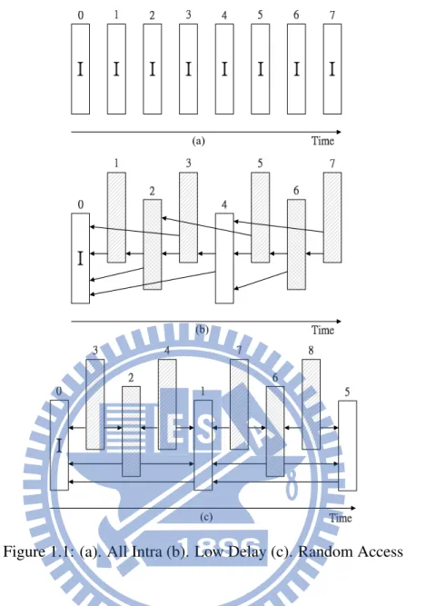
Three types of situations have also been established to be used for different applications in HEVC. All-Intra (AI), Random Access (RA), and Low Delay (LD) are defined for different
(a)
(b)
(c)
Figure 1.1: (a). All Intra (b). Low Delay (c). Random Access
usage. All-Intra is used for all frames which are intra coded without using temporal domain frames as shown in Figure 1.1 (a). The number on the frame of top is encoding order. Low Delay is for the real time communication with least encoding delay, only the first frame is intra coded, the others are P or B frames using inter prediction as shown in Figure 1.1 (b). Random Access is used for hierarchical structure and I frame is put in the group of pictures periodi-cally, and the encoding order follows the I frame first and then the P/B frames as shown in Figure1.1(c).
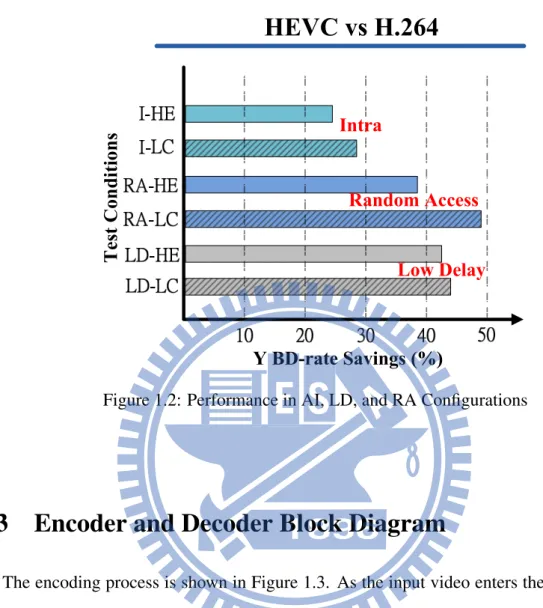
The bit-rate saving performance compared with H.264/AVC between each configuration is shown in Figure 1.2 . In this Figure 1.2, we can see that All Intra has little coding gain at almost 28 percent, the most powerful case is random access in the high efficiency condition
which can achieve almost 50 percent reduction in bit-rate savings. All the configurations can achieve better bit-rate performance than H.264/AVC.
Intra
Random Access
Low Delay
Y BD-rate Savings (%)
HEVC vs H.264
T
e
st
C
o
n
d
iti
o
n
s
Figure 1.2: Performance in AI, LD, and RA Configurations
1.3
Encoder and Decoder Block Diagram
The encoding process is shown in Figure 1.3. As the input video enters the video encoder, the output will be the binary bit-streams. The encoder is composed of three main parts, one is prediction stage, another is texture coding, and the other is binarization coding. In the pre-diction stage, intra prepre-diction and motion estimation which are the main contributions in the compression standard are to predict the frames based on the spatial locality and the temporal domain including back and forth. After the predicted frames are produced by one of the predict engines, the output of the minus operation on the original frames and the predicted frames are so called residual data. Residual data then enters into transform coding from the un-apparently the spatial domain to the frequency domain. Due to human eyes insensitivity to high frequency, the data can be quantized and discarded to reduce the reluctant data. Finally, the remaining data will enter into the binarization, entropy encoding process. The purpose of the entropy encoder
is to encode the symbols from other modules to the bit-streams. To point why the encoder has the embedded decoder is that due to avoiding the mismatch between encoder/decoder side, the inverse quantization and inverse transform are to reconstruct the residual data. The predicted frames would add with residual data and become reconstructed frames. Due to the motion compensation, reconstructed frames need to match in order to synchronize with encoder and decoder side. Because of the block-based coding, artificial block effect produced by the in-tra/inter prediction and discrete transform coding, will harm the video quality. Therefore, the filter stage including deblocking filter, sample adaptive offset and adaptive loop filter are to smooth the block edge between boundaries to improve the video quality. The decoder side is
Quad Tree Structure Intra Prediction Motion Compensation
-Predicted Frame Motion Estimation Transform Quantization Inverse Quantization Inverse Transform De-blocking Filter
SAO & ALF Frame Buffer Embedded Decoder B its tr e a m E n tr o p y E n c o d e r
shown in Figure 1.4 , the main component parts are the same as the encoder. The bit-streams enter into the entropy decoder and produce the syntax symbols and the transform coefficients. The prediction stage and transform coding will be reconstructed by utilizing the synchronous adders. Due to the block edge effect, the in-loop filters are used to improve the video quality in order to smooth the visual badness.
Entropy Decoder Motion Compensat ion Inverse Quantizati on Inverse Transform Intra Prediction De-blocking Filter SAO & ALF
Figure 1.4: Video Decoder Diagram
1.4
Coding Features
HEVC has fruitful novel coding tools different from H.264/AVC described in last section. In entropy coder, the Context Adaptive Binary Arithmetic Coding (CABAC) is still contained in HEVC while the CAVLC is displaced. Due to the high data dependency, the throughput of the entropy coder is limited insufficiently for hardware implementation due to the running frequency. Therefore, the HEVC has adopted a novel technique wavefront parallel processing (WPP) which can break out the strong data dependency to improve the system throughput. In the prediction stage, due to the flexible block size partition, the inter prediction has adopted advanced motion vector (MV) prediction not only from the neighboring blocks. Moreover, the DCT-based interpolated filter and motion merge group (MRG) sharing all motion parameters in the adjacent blocks are the main features in inter prediction. In the intra prediction, its angular prediction and adaptive pre-filtering also enhance the prediction accuracy in order to remove
more the redundancy. Furthermore, the transform coding structure contains the discrete cosine transform and discrete sine transform to efficiently transform the residuals in to frequency do-main. Because of the multiple block-based partition in HEVC, after the reconstruction between transform coding and prediction stage, the artificial defect will be more apparently shown be-tween the block edges. As a result, to further improve quality, the loop filter adds two coding tools sample adaptive offset (SAO) and adaptive loop filter (ALF). The novel filters contain adding offsets and adopting adaptive filter coefficients. The coding tool features will be de-scribed in detail in next sections.
1.4.1
Coding Tree Unit Structure
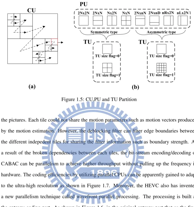
The emerging HEVC standard has adopted flexible block partitions, the coding tree ap-proach in HEVC has brought coding efficiency better than previous standard. In addition, the block size not only supports 16x16 but also enlarges 64x64 with more efficient flexibility. A slice contains multiple coding tree units (CTU) like macroblock in prior standard H.264/AVC. It follows the double z scan order from left to right and top to down in the quad-tree based partitions as shown in Figure 1.5 (a). The CTU has been further split into multiple coding units (CU) recursively. The prediction unit (PU) is contained in the CU, the PU is adopted for in-ter/intra prediction with more efficient prediction and also can improve the coding accuracy as shown in Figure 1.5 (b). The main part for having better bit-rate reduction is adopted quad-tree PU partitions. Transform unit is for discrete cosine transform, it includes which will decide whether to further split or not.
1.4.2
High Level Parallelism
In the HEVC, the picture is split into many independent tiles which consist of multiple Largest Coding Units (LCU). The shape of tiles can be rectangular or square, or the number of tiles can be only on or several LCUs. The coding order of the tile is adopted as raster scan order, also the internal tiles of LCUs are raster scan order too. The concept of tile is like the slice in
PU
CU
2Nx2N 2NxN Nx2N NxN 2NxnN 2NxnD nRx2N nLx2NSymmetric type Asymmetric type
TU size flag=0 TU size flag=1 TU size flag=0 TU size flag=1
TU
TU
(a)
(b)
Figure 1.5: CU,PU and TU Partition
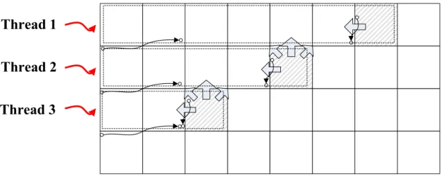
the pictures. Each tile could not share the motion parameters such as motion vectors produced by the motion estimation. However, the deblocking filter can filter edge boundaries between the different indepedent tiles for sharing the filter information such as boundary strength. As a result of the broken dependencies between each tiles, the bit-stream encoding/decoding of CABAC can be parallelism to achieve higher throughput without pulling up the frequency in hardware. The coding efficiencies by utilizing parallel CPUs can be apparently gained to adapt to the ultra-high resolution as shown in Figure 1.7. Moreover, the HEVC also has invented a new parallelism technique called wavefront parallel processing. The processing is built at the entropy coding part. As shown in Figure 1.6, in the original entropy part that as the final LCU has finished the coding, the next line of the first LCU can start to encode. Therefore, the strong data dependency tied the throughput of the entropy part. But in the HEVC, the Figure 1.6 points that the entropy coder at the next new line can begin when the top line of 2 LCUs have already been finished. The data dependency would not be followed at the end of the line LCU. Therefore, the multi-thread could enhance the degree of parallelism to improve the throughput and frame rate.
Thread 1
Thread 2
Thread 3
Figure 1.6: Wavefront Parallel Processing in Entropy Coding
Tile #1
Core 1
Tile #2
Core 2
Tile #1
Core 1
Tile #2
Core 2
Tile #3
Core 3
Tile #4
Core 4
Figure 1.7: Tiles Processing in Multi-Core
1.5
Motivation and Design Challenges
Intra prediction uses spatial correlation to remove the pixel redundancy. At the same time, intra prediction need to utilize the neighboring pixels including upper side and left side. In terms of the video decoder, the neighboring pixels used for intra prediction must be un-filtered before deblocking filter. As a result, with block-based coding in intra prediction, the bottom line of predicted pixels after the reconstruction with IQ/IT needs to be saved due to the lower boundary blocks unavailable. Therefore, the upper line pixels which the line buffer with size of frame width should be stored in the hardware design. Consequently, the intra prediction requires 1 line buffer. Also, deblocking filter’s processing order is the same as H.264/AVC, that means vertical edge first and then horizontal edge to gurantee the block boundary is smoothed.
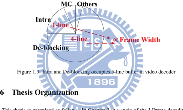
However, in the HM-7.0 reference software design, deblocking filter uses frame-based level coding while it requires large frame buffers storage without concerning the hardware cost and implementation difficulties. This is inefficient in the architecture design, so the macroblock-based coding is likewise adopted in deblocking filter. Therefore, with block-macroblock-based design, the upper 4 lines filtered pixels which are the neighboring pixels for the deblocking filter should be loaded from the line buffers. After finishing vertical edge filtering, the bottom 4 lines of output filtered pixels would be written back to the 4-line buffers with size still depends on the frame width. Certainly, in the video decoder system, 5 line buffers all depending on the frame width occupy a great portion of the internal memory in the chip area. In spite of achieving lower bit rate compared with H.264 standard with same video quality in HEVC, the coding tools still require the higher hardware cost including memory size, power consumption and chip area. In the mean time, the analysis of the memory requirement for each resolutions shown in Figure 1.8 illustrates that although the storage for deblocking filter dominates the great amount of memory size in the video decoder, intra prediction still occupies almost 15% to 20% percent parts in the higher resolution. Also, in the Ultra-HD resolution, up to 15.36K byte memory is required. Consequently, the equation 1.1 depicts that the whole memory requirements in the video decoder system for the YCbCr (4:2:0). The memory profiling shown in Figure 1.9 is also described that the decoder memory is dominated by the intra predictor and the deblocking filter. Due to the line buffers for intra prediction and deblocking filter are dependent on the frame width, total memory requirement is dominated by intra prediction and deblocking filter. Naturally, how to reduce the line buffers of intra prediction for almost 20 percent memory reduction in the video decoder is an important issue and motivation. Moreover, the memory reduction of the deblocking filter is also important issue in the hardware design.
QCIF CIF HD 720 Full HD Quad HD Ultra HD 10K 20K 30K 40K Total SRAM 38K-Byte
Figure 1.8: Total SRAMs in Video Decoder with Different Resolution
Intra
MC
De-blocking
Others
1-line
4-line
Frame Width
Figure 1.9: Intra and De-blocking occupies 5-line buffer in video decoder
1.6
Thesis Organization
This thesis is organized as follows. In Chapter 2, we study of the I-Frame decoding flow including entropy coding, intra prediction, inverse transform and in-loop filter for the newest standard HEVC and the previous work of the memory reduction will also be stated. Chapter 3 will first introduce the proposed algorithm and compares performance with previous designs. Chapter 4 gives the hardware architecture of the I-Frame decoder system with wavefront parallel processing. Chapter 5 presents implementation results, verification and performance evaluation to verify the hardware design. Finally, conclusions and future works are given in Chapter 6.
Chapter 2
Study of the I Frame Decoding Flow
The study of the I frame decoder will be detail described in this chapter. The I frame decoder of our work shown in Figure 2.1 consists of intra prediction, inverse transform coder, and in-loop filter. The algorithm of each components toward HEVC will be explained later. However, in the low resolution long time ago such as MPEG-1 or MPEG-2, the memory requirement problem is not apparent in the hardware design. However, the applications of HEVC is toward the Quad Full-HD TV, therefore, the memory requirements of the intra prediction and deblocking filter will rise up inefficiently to waste power consumption and area efficiency. In the approaches of [1] and [2], their designs use the external memory and exploit memory hierarchy to decrease the internal memories. The summary would talk about the deficiencies of their designs. The sections below would describe the video component of each functionalities detaily as shown in Figure 2.1. Inverse Quantization Inverse Transform Intra Prediction De-blocking Filter SAO & ALF Texture Decoding In-loop Filtering Pixel Prediction Bitstream Decoding
2.1
Entropy Decoder
The purpose of the entropy coding is to encode the syntax elements of the video streams in a compressed binary sequence for easily transmittion over the internet or any cable. The elements include the transform coefficients after the DCT and zig-zag scan order, motion vectors which are defined as the difference coordinate of the candidate block and current block, and some picture, slice and block level headers. The elements will be encoded as fixed or variable length binary codes or context-adaptive binary codes based on the element types. When the entropy coding mode equals 0, the transform coefficients will be encoded as context-adaptive variable length coding (CAVLC) by using run-level coding to represent continuous zeros. If the previous elements after zig-zag scan order are numerous 1 or negative 1, the CAVLC will use compact ways to represent 1 or negative 1. Moreover, the non-zero coefficients have strong correlation in the neighboring blocks and the coefficients will be encoded by utilizing look-up table.If the encode coding mode equals 1, the CABAC has better compression performance by adaptively choosing the element probability model. The probability models will adaptively change based on the element contexts. As shown in Figure 2.2, the binary bitstreams will firstly binary arithmetic decode and output the non-binary information bin. Secondly, the context model will update the probability depending on the bins which will be binarized into binary code. If the binary codes are numerous 1s, then the probability will be higher. In the HEVC, the throughput is higher than H.264/AVC due to the following improvements, breaking the model dependencies, grouping the bypass bins and reducing coded bins.
Binarization Regular Decoding Engine Bypass Decoding Engine bypass normal bit stream Binary Arithmetic Deoder loop over bins bin strin g syntax element Context Modeler bin bin bin strin g bin
2.2
Intra Prediction
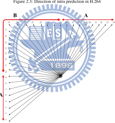
In the intra prediction, it is one of the important prediction engines in the video coding stan-dard. Since in the H.264/AVC standard, the intra prediction is adopted to improve the spatial redundancy. When the previous frame changed abruptly, like scene change, therefore, the tem-poral domain prediction will not guarantee the prediction accuracy. Unfortuntely, it may cause the bit-rate higher and would transmit the prediction error. The purpose of the intra prediction is to help the temporal domain prediction to compromise the scene change. Normally, the period of the intra prediction in the group of pictures is the first one every IPPBIPPB or randomly in-sert an I frame to shut down the error propagation induced by the temporal prediction. With the help of the intra prediction, the H.264/AVC can achieve the hottest video applications during the last decade. In HEVC, the call for proposal during the meeting aims to enhance the bit-rate savings. Therefore, the intra prediction is urgently to further improve the prediction accuracy than previous standard in H.264/AVC. The mode of intra prediction is an important issue to be discussed. In H.264/AVC, the specification defines 9 modes for the 4x4 block, intra 4x4, 4 modes for 16x16 block, intra 16x16 as shown in Figure 2.3. The concept of the intra prediction is to use neighboring pixels to predict the current block. Therefore, the modes in H.264/AVC are sufficiently to predict frames from top, left, to right top corners. However, if the required resolution is Ultra-HD or more, the prediction accuracy for the intra prediction apparently is in-sufficient. Accordingly, the MPEG team aims to add more modes to further improve the coding efficiency and gain more bit-rate savings. In the specification of HEVC, the modes are defined as 35 more than previous standard as shown in Figure 2.4. Certainly, the results of the predicted frames are more precisely than before. The basic concept of the spatial domain prediction is to utilize the neighboring pixels including top and left reference pixels. The Table 2.1 shows that intra mode number corresponding to the associated names.
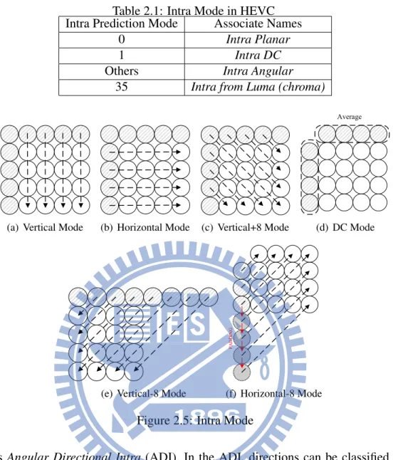
In the mode number 1, Intra DC is to average the top row and left column reference pixels same as the H.264/AVC. In addition, the HEVC standard defines the DC post filtering in order to smooth the blocky effect as shown in Figure 2.5(d). In the direct mapping mode such as vertical,
1
0
4
3
6
8
5
7
Figure 2.3: Direction of intra prediction in H.264
17 1 6 1 5 1 4 1 3 1 2 11 1 0 9 8 7 6 5 4 3 2 18 19 20 21 22 23 24 25 26 27 28 29 30 31 32 33 34
A
A
B
Figure 2.4: Direction of intra prediction in H.265
horizontal, diagonal from top right, bottom left and top left are the same as H.264/AVC. In the horizontal-8 mode, if the pixels are unavailable, the pixels are the padding. Also, in order to reduce the blocky effect, after the vertical and horizontal prediction, the post filter between boundary is filtered with predicted pixels and neighboring pixels.In the mode range of 2-34, is
Table 2.1: Intra Mode in HEVC
Intra Prediction Mode Associate Names
0 Intra Planar
1 Intra DC
Others Intra Angular
35 Intra from Luma (chroma)
(a) Vertical Mode (b) Horizontal Mode (c) Vertical+8 Mode
Average
(d) DC Mode
(e) Vertical-8 Mode
P A D D IN G (f) Horizontal-8 Mode
Figure 2.5: Intra Mode
named as Angular Directional Intra (ADI). In the ADI, directions can be classified into two groups. As shown in Figure2.4, the group A uses positive angles while group B uses negative angles. The positive prediction angles have the range from [2, 5, 9, 13, 1, 7, 21, 26], 0 and 32 angles are the direct mapping in the vertical+8, vertical-8 and horizontak-8. The angle is defined as the displacement of the current pixel and top reference pixel in the vertical prediction. Also, it is defined as the right current pixel and left column pixel in the horizontal prediction. We first describe the group A of intra prediction in detail. In Figure 2.6, take mode 27 for example, the current 4x4 block only needs top reference pixels. Different with H.264/AVC, the current predicted pixel needs two inputs to do the linear interpolation. According to the specification, the choice of the two pixels is adopted the angle calculation. As shown in Figure 2.6, the parameter P OS0 will be added with angles which would be achieved by the look-up
table to get P OS1, then P OS1 will next to be added with the same angles to get the P OS2.
After finishing angle operations, the output of the intra prediction pixel is calculated in 32-tap filtering. If the angles are negative, then the Table2.2 shows the negative angels corresponding to the inverse angles. The processing step to do the intra prediction in negative angles is to first flip the pixels from the side to the main as shown in Figure 2.7(a). Also, the pixel decision is through the look-up table and then do the interpolation as the same as Figure 2.6.
C A B POS0 POS1 POS2 POS3 an g le A C B 32-POS0 POS0 an g le an g le interpolate
Figure 2.6: 4x4 block interpolation of intra prediction
Table 2.2: Intra Inverse Angles in HEVC
Intra Prediction Mode 2 3 4 5 6 7 8 9
inv Angle -256 -315 -390 -482 -630 -910 -1638 4096
Intra Prediction Mode 19 20 21 22 23 24 25 26
inv Angle -315 -390 -482 -630 -910 -1638 4096
(a) flip the pixels (b) inverse angle filtering
Figure 2.7: Inverse Angle
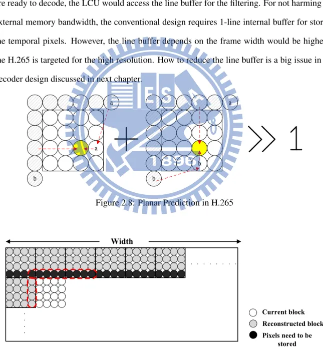
To gain the benefit of the homogeneous region in the I frame, HEVC proposed the new planar mode interpolation. As shown in Figure 2.8, the planar operation requires two steps. In the left filtering, pixel a is copied to the rightmost of the current pixel, the leftmost of the pixel
is linear operation with pixel a. In the right filtering, the pixel b is also put in the bottommost of the current pixel, the topmost pixel is linear operation with the pixel b. Finally, the bilinear filtering will get the planar output. In concept of the intra prediction algorithm, it requires top row and left column pixels for the input filtering. Further, in the hardware-based design, the coding order follows the raster scan order. Because the next line of LCUs are not available when decoding the first line of LCUs. Accordingly, the intra predicted pixels after the recon-struction with transform data should be stored into the line memory. As the next line of LCUs are ready to decode, the LCU would access the line buffer for the filtering. For not harming the external memory bandwidth, the conventional design requires 1-line internal buffer for storing the temporal pixels. However, the line buffer depends on the frame width would be higher if the H.265 is targeted for the high resolution. How to reduce the line buffer is a big issue in the decoder design discussed in next chapter.
Figure 2.8: Planar Prediction in H.265
Current block Reconstructed block
Width
Pixels need to be stored
2.3
Transform Coding
Transform coding is widely adopted in video coding to compress the redundant data. As the predicted pixels minus with original pixels in the encoder side, the residual data will be transformed from the spatial domain into frequency domain. Due to the human eyes sensitive in the low frequency, the data in the high frequency can be quantized to discard information so as to compress video data. The transform in H.264/AVC adopts 3 types depending on the intra mode and size. Hadamard transform for 4x4 array of luma DC coefficients in intra macroblock predicted in 16x16 mode. Hadamard transform for 2x2 chroma block and DCT-based transform in 4x4 block. The advantage of the DCT/IDCT in H.264/AVC is that it adopts integer transform which can possibly no mismatch happened in encoder/decoder side. In addition, the core of the transform can be implemented using only shift and additions. While the transform in HEVC has increased up to 32-point transform matrix. Here, the 4-point and 8-point are shown in equation 2.1 and 2.2. The properties of HEVC transform are that the odd rows are even symmetric and even rows are odd symmetric. Moreover, the elements in the smaller transform matrix are also the elements of larger transform. The bold words are also the elements of 4-point transform matrix. The properties make hardware easily implement.
H = 64 64 64 64 83 36 −36 −83 64 −64 −64 64 36 −83 83 −36 (2.1)
H = 64 64 64 64 64 64 64 64 89 75 50 18 −18 −50 −75 −89 83 36 −36 −83 −83 −36 36 83 75 −18 −86 −50 50 86 18 −75 64 −64 −64 64 64 −64 −64 64 50 −89 18 75 −75 −18 89 −50 36 −83 83 −36 −36 83 −83 36 18 −50 75 −89 89 −75 50 −18 (2.2)
2.4
In-Loop Filter
Due to the block-based coding structure adopted in the video compression standard, the dis-continuities between the block edge cause the blocking effect. The major source of the blocking effect comes from the prediction stage, transform coding and quantization step. Due to the mul-tiple shapes inter blocks adopted during the H.264/AVC and HEVC, the block discontinuities exist followed by the predicted block. Also, the transform coding adopted block-based split structure, the inverse discrete cosine transform cannot recover back the transform coefficient completely in the decoder side. Moreover, in the quantization process, the step of the transform coefficient aims to reduce the high frequency redundancy. However, in the reverse quantization which is also called the scaling process cannot scale back completely. Above the reasons, the MPEG team proposed filters which can smooth the blocking effect between block boundaries. Three types of the filters, one is traditional deblocking filter, another is sample adaptive offset which would add offset to the deblocked pixels, the other is adaptive loop filter which utilize the adaptive filter coefficients in the encoder side, they are adopted in the HEVC which already improved the video quality better than previous standard H.264/AVC.
2.4.1
Deblocking Filter
The differences of H.264/AVC and HEVC in deblocking filter are shown in Table 2.3. In the filter size, H.264/AVC adopted 4x4 filter size to guarantee that every edge would be smoothed. In contrast to the H.264/AVC, being suitable for the high resolution, if the filter edge is still 4x4 size then the complexity and coding time will be sufficiently large than H.264/AVC. Ac-cordingly, the HEVC decided to filter in 8x8 size not only to support larger resolution but also enhances the coding efficiency. Moreover, to reduce the complexity in software/hardware im-plementations, the boundary strength of the deblocking filter decreases to 0∼2. 0 means to skip the deblocking filter, 1 means normal edge effect, 2 means strongest edge effect. In the filtering order, it is the same as H.264/AVC from vertical edge first and then horizontal edge in the LCU. The coding feature of the HEVC comes from the highly parallelism, wavefront processing and tiles. In the deblocking filter stage, the parallelism is also adopted to improve the coding effi-ciency. It still keeps the data dependency which is caused in the filtering order, vertical edge first and then horizontal edge. In the software-based implementation, the deblocking filter op-erates vertical edge filtering in the frame-level and then horizontal edge filtering will start after the frame finished vertical edge filtering. This frame-level parallelism makes deblocking filter more efficient and more fast while the strong data dependency has been broken down. The main differences about the in-loop filter in H.264/AVC is that HEVC creates two coding mod-ules to further improve the video quality, the sample adaptive offset which will first classify the deblocked signals and add the specified offsets to the group signals, the other is adaptive loop filter, it uses wiener filter to decrease the mean sum error between the original data and filtered data, the multiple shapes of the filter are its advantage to flexibly merge into each region. The details of the algorithm will be discussed later.
The blocking effect which is caused by the block-based coding unit is easily noticed by the human eyes. However, not every block edge should be smoothed by the deblocking filter. Re-dundant smoothing will cause the frame fuzzing, also cause the coding inefficiently. Therefore,
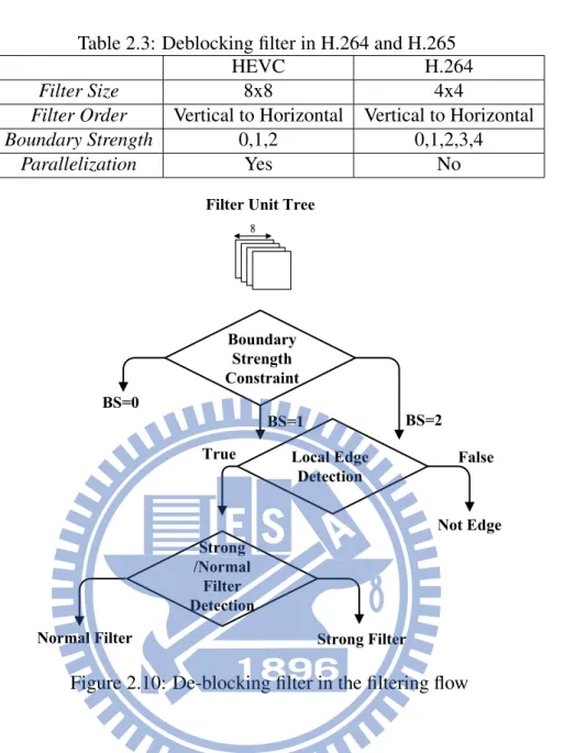
Table 2.3: Deblocking filter in H.264 and H.265
HEVC H.264
Filter Size 8x8 4x4
Filter Order Vertical to Horizontal Vertical to Horizontal
Boundary Strength 0,1,2 0,1,2,3,4 Parallelization Yes No Boundary Strength Constraint Local Edge Detection BS=2 BS=1 BS=0 Not Edge False True Strong /Normal Filter Detection Strong Filter Normal Filter
Filter Unit Tree
Figure 2.10: De-blocking filter in the filtering flow
the decision stage before filtering is vital to the deblocking filter. The filtering stage is classi-fied for 3 steps, one is boundary strength calculation, another is local edge detection and the other is normal/strong filter decision as shown in Figure 2.10. In the boundary strength classi-fication, the strength number means how strong the blocking effect arise on the block edge. In H.264/AVC, the strength number counts for 0∼4. In HEVC, in order to achieve low complexity, the strength number is reduced to 0∼2. In Table 2.4, the filter condition is that if the samples in the block meet the condition, then it corresponds to the boundary strength. In 2, if the sam-ples in the block are intra coded, then the block effect is the strongest which means the edge is over-sharped. In 1, if the samples of block p or q in a block unit has non-zero transform coef-ficient and boundary is transform unit or use different reference pictures or different number of
Table 2.4: Deblocking filter boundary strength in H.265
Filter Condition Boundary Strength
The sampls p or q in a coding unit
2 is intra prediction
The sampls p or q in a coding unit
1 non-zero tranform coefficients and
boundary is transform unit or use different reference pictures or different
number of motion vectors
Others 0
motion vectors, then the edge is normal effect often seen in the P or B frames. Otherwise, the deblocking filter is skipped for maintaining the edge contents. After the boundary strength is decided, if it is greater than 0, the following local edge detection is performed. In the local edge detection, its purpose is to guarantee whether the edge is exactly existed or not. In the Figure 2.11, the P block and Q block is 4x4 block size, and the equations of (1)∼(3) are the detection process. The dp0 is following the sobel operation to achieve the operation results. After the sum
16 d c b a P block Q block dp0 dp3 dq3 dq0 a b c d e f g h Current Available dp0=a-2*b+c (1) Sum=dp0+dp3+dq0+dq3 (2) If(Sum<beta(QP)) (3) Filter On
Figure 2.11: Operation in deciding the filter on
of the dp0, dp3, dq0, dq3 in the P or Q block, the comparison with the beta and sum will decide whether the edge would be filtered or not. The parameter beta is dependent on the quantization step Q. The listed Q and beta are shown in the HM-7.1 reference software. As the sum is less
than beta, then the filter is actually on. Summarily speaking, the deblocking filter is almost the same function of the previous standard with less hardware complexity.
2.4.2
Sample Adaptive Offset
In the sample adaptive offset, the main point is to further reduce the distortion of the de-blocked pixels. The concept of the sample adaptive offset is to classify the reconstructed pixels into multiple categories. Each category corresponds to different offset. After the specified classification, the offset finally adds with the deblocked pixels. The offset of each region and classification type will be coded into the bitstreams. The HM-7.1 reference software reported that SAO achieves 3.5 percent bit-rate reduction and up to 23.5 percent bit-rate reduction with less than 1 percent encoding time increase. The followings are going to describe the algorithm of classifications in the SAO. The offset may differ sample by sample in the same region. In the low complexity configuration, two types of classifications are adopted in HEVC. The first is Edge Offset, the other is Band Offset. In the Band Offset, the main method of classification is to separate the pixels by the gray-level intensity into multiple regions as shown in Figure 2.12. In the 8 bits of gray-level, it ranges from 0 to 255, each sample will be classified into one
Minimum sample
value
Maximum sample
value
sample intensity
Figure 2.12: Sample Classification in HEVC
region. Therefore, the region of width is 8, totally 32 regions will separate the signals from low intensity to high intensity. In the Figure2.13, the dotted line is original curve, the dash line is the distortion curve which has to be added with offset to pull back the curve. In the bank k and k+2, the positive offset is to pull up the distortion curves to the almost original curves, and in the bank k+1, the negative offset is to pull down the over-intensity signals to the appropriate curves. Besides, the region of index and offset will be signaled to the decoder to lessen the burden of
band k
band k+1 band k+2
sa
m
p
le
v
a
lu
e
POSITIVE
OFFSET
POSITIVE
OFFSET
NEGATIVE
OFFSET
Distortion curves
Original curves
Figure 2.13: Sample Classification in HEVCthe coding complexity. In the Edge Offset, the purpose is to compare with neighboring pixels as shown in Figure 2.14. There are 5 categories which are listed in Table 2.5. In the category 1,
Figure 2.14: SAO Edge Offset Type in 4 mode
Table 2.5: Edge Offset Category
Category Condition
1 c<2 neighbors
2 c<1 neighbor and c==1 neighbor
3 c>1 neighbor and c==1 neighbor
4 c>2 neighbors
0 None of the above
if two neighbors are larger than current pixel c, then positive offset will be added to pull up the intensity level. In the category 2, if the condition is true, then the positive offset is also added. In the category 3 and 4, the negative offset are going to pull down the current pixel to smooth the pixel value. As shown in Figure 2.15, the positive offset in the 1, 2 and 3 are shown to pull
up the over-low intensity between the left and right pixels. In addition, the negative offset in the 3, 4 and 5 are to pull down the over-high intensity signals.
n1 c n2 Sample value Category 1 n1 c n2 Sample value Category 2 n1 c n2 Sample value Category 2 n1 c n2 Sample value Category 4 n1 c n2 Sample value Category 3 n1 c n2 Sample value Category 3 POSITIVE OFFSET NEGATIVE OFFSET
Figure 2.15: SAO Offset type
2.4.3
Adaptive Loop Filter
The Adaptive Loop Filter of the incoming video standard HEVC is adopted in the in-loop filter of the final stage. It is applied after the deblocking filter and sample adaptive offset in order to further reduce distortion compared with original frame. Its innovation is to use Wiener filter to reduce Mean Square Error related to the reconstructed frames. The algorithm of the Wiener filter filter out the signals which are already polluted. Based on the communication theory, the MMSE estimator is built on the wiener filter coefficient construction. The coefficients generated by the Wiener filter are adaptive to the pixel content region. It means that in the encoder, the loop of the producing filter coefficients is the time consuming due to the pixel content variable. In the encoder, over 40% of the time is on the statistic data gathering. Therefore, the reduced time complexity is a big issue in the implementation. The Figure 2.16 shown below is to describe the differences between the original frame and the reconstructed frame should be the least during the recursively wiener filter coding loop. The filter shape has multiple 2 dimensional filters with cross diagonal. In the encoder side, the filter unit splitting is complete with recursive structure. The Figure2.17 shown below is that the filter on/off is encoded recursively with quad-tree structure. Also, the encoded parameters including filter on/off and filter coefficients
Original Frame
e(n)
SAO
Output Frame
Figure 2.16: ALF Concept
will be signaled to the decoder to lessen the decoder complexity. In the cross filter shape, as shown in Figure 2.18. The number in the block means the same coefficient index which means that as the product of the coefficient and the pixel value, the sum of the products would finally clip to the appropriate value. The ALF in the decoder side is as described follows. First, parse
Figure 2.17: ALFOn or Off
the syntax element from the entropy decoder from the bitstream to decode the partition diagram which is filter on/off and also construct the filter coefficients and the filter type. Second, map the filter parameters into pixel regions to reconstruct the filter outputs. Thirdly, store the filtered pixels to the temporary buffers because the filtered pixels would not be the filter input.
0
1
3
9
3
1
0
4
2
2
4
8
7
8
6
5
5
6
7
Figure 2.18: ALF filter shape
2.5
Related Works of the Low Memory Architecture
The intra predictor and in-loop filter are the memory dominated coding tools in the video decoder system. There are total 5 line buffers all depending on the frame width which occupies a great portion of the internal memory in the chip area. In spite of high coding efficiency in HEVC, the coding modules still require the higher hardware cost including memory size, power consumption and chip area. In the meantime, the memory requirement for the video decoder hurts the performance of the I frame decoder. In the intra prediction, it originally occupies almost 15∼20 percent parts in the higher resolution. Also, in the Ultra-HD resolution, up to 8 Kbytes memory are required. For the deblocking filter, the macroblock-based coding results the bottom 4 line of pixels not horizontal filtered. Therefore, the 4 line of pixels should be stored for the next new line of LCU is ready. Consequently, in the next section, the traditional approaches are aimed at discussing the intra prediction and deblocking filter memory usage. Due to the line buffers for intra prediction and deblocking filter are dependent on the frame width, total memory requirement is dominated by intra prediction and deblocking filter. Naturally, how to reduce the line buffer of intra prediction for almost 20 percent memory reduction and also the 75% deblocking filter memory in the video decoder are important issue and motivation.
2.5.1
Traditional Approaches
The memory in the design [3] is aimed at HD real-time decoding which the intra predictor uses size of frame width with BRAM cache to store the data. The main contribution of the [4] is to enhance the maximum throughput, which can reach 1991Mpixles/s for 7680x4320p. How-ever, the memory for the intra predictor requires almost 15Kbytes which occupies the core chip area 20 percent. In the traditional approaches of the intra predictor, almost all designs use 1-line buffer to store the data.
For the deblocking filter approach, the design of the [5] has declared two SRAMs, the one is 144x32 bits single-port SRAM, the other is 16x32 bits two-port SRAM, also they exploit group-of-pixel in the memory store instead of column-group-of-pixel or row-group-of-pixel. Also the other work of the [6] has required two-port 160x32 bits SRAM to store the current macroblock and adjacent temporary filtered pixels. The design utilizes bus-interleaved [7] to improve 7x performance throughput while they exploit the emulated ARM cpu and embedded SRAM with size 96x32. The work also utilizes three on-chip SRAM modules to store the luma, cb and cr data in the [8]. Also, the architecture uses two-port SRAMs with size 16x32 in [9]. However, the external memory bandwidth problem did not make point to solve. Therefore, make all the pixels out of the chip memory is not a good solution for the deblocking filter. Above designs although did not use 4-line buffers to store the temporary data, the external memory bandwidth is a serious problem happened in the system. External memory bandwidth causes power consumption and also reduce the system throughput. In [10], the design requires frame size data buffer for storing the Line-of-Pixel(LOP). Therefore, the 4-line data buffer is huge compared with above designs which take on-chip SRAMs off the chip, but it does not need any external memory bandwidth. In most designs in intra predictor and deblocking filter, they did not analyze the trade-off with the external memory bandwidth and the internal memory requirement. Some of designs target for the content buffer only using external memory, while others use frame-dependent size mem-ory to neglect the SRAM size wasting. The next section will describe the methods to reduce internal memory with the system viewpoint considering the power consumption and also the
memory bandwidth.
2.5.2
Line-Pixel Lookahead
The design improves the memory hierarchy and reduce the embedded SRAMs for the intra prediction, deblocking filter for achieving low power consumption in the [1]. The design aims at copying the correlated data from larger memories which has high data-correlation to the smaller memories. This concept enhances the access time latency and the embedded SRAM could be set smaller with appropriate hit rate. The memory hierarchy adopts three-level including the content, slice and DRAM. The slice memory allocates the all row reconstructed pixels for the intra prediction and vertical filtered pixels for the deblocking filter. Further, they also proposed the line-pixel-lookahead to eliminate the un-used pixels. The main idea of LPL scheme is to
Figure 2.19: Line pixel lookahead [1]
utilize spatial locality in the vertical direction, and looks ahead before decoding the next line of pixels [1]. Not all the neighboring pixels should be kept in the internal memory for vertical direction locality, most pixels are following the vertical mode similarity. A reduced embedded SRAM stores the pixels in the above LCUs and the LPL scheme is to predict whether the pixels would be stored in to the SRAM or not. Most pixels are determined as a horizontal-related
required to record each prediction tag and perceive the contrast between Neighboring TAG and Decoding TAG. The deblocking filter and intra predictor generates corresponding TAG information to forecast whether the next line of pixel should be kept or not. To reduce the size of memory, the Figure2.19 is exploited to reduce the miss rate. One OR gate, five comparators, two multiplexers and inverter are used to implement [1]
2.5.3
DMA-like Buffer
The purpose of the DMA-like buffer is to store the correlated data in a MB in the external memory if they are not used immediately [2]. Using the DMA-like buffer, the internal memory can be reduced from 26K in 1080p resolution to only 0.5K bytes, which results in 98 percent reduction in memory size. For the dual external memories adopted in the design to reduce the required clock rate for memory access operations. With less than 10 percent increase in external memory bandwidth, the trade-off between internal memory and external memory bandwidth provides flexibility for system designers. However, in the Figure 2.20, about 83.4MB/s of external memory bandwidth occupies the 9.5 percent in total 878MB/s by using this technique. If the power consumption is calculated utilizing Micron Power Calculator, the result is 33.9mW, which is larger than [1]. As a result, it is not good to put the almost internal data off the chip.
2.6
Summary
Therefore, in the proposed algorithm, the memory would not totally cut into the off-chip memory. Also, the proposed I frame decoder is composed of the inverse discrete transform, intra predictor and in-loop filter which will be prototyped in FPGA platform and demo the video in the verification mechanism. Besides, in the next proposed algorithm, the proposed method can further achieve lower memory size with higher hit rate based on the memory hierarchy architecture compared with [1]. With the system pointview, the proposed method has better performance including memory access power consumption, external memory bandwidth and miss rate. The next chapter will describe the algorithm in detail.
Chapter 3
Proposed Algorithm
Due to the algorithm of HEVC, the on chip memory is required for the hardware to use. The huge on chip memory will cause the power consumption and waste the chip area efficiency. According to the conclusion summarized in section 2.6, that the traditional approaches are com-monly using internal line buffers to store the un-filtered pixels for intra prediction and filtered pixels for in-loop filters.
3.1
Above Line Buffer Sharing
For system viewpoint, the intra predictor and deblocking filter in video codec are the mem-ory dominated modules. In the hardware design concept, the correlated pixels need to be stored into the line buffers for waiting the next line of LCUs are available. For intra prediction, the reconstructed pixels stored into line buffer should be in the previous in-loop filter stage. The deblocking filter utilizes 4-line buffers to store the pixels which are filtered in vertical edge only as shown in Figure 3.1. The pixels would be used since the horizontal edge is started for the next new line LCUs are available. Therefore, the notification of the memory accesses would be impact to the hardware design. The concept of reducing internal memory in above line buffer sharing is to schedule the data path between intra prediction and deblocking filter. In Figure 3.2, the 4-line buffer is composed of two parts, one is original line buffer which saves the
re-constructed pixels for the intra predictor to use, and the other parts 3-line buffer is saving the vertical edge filtered pixels for the deblocking filter to use. The details of data scheduling will be described in the Algorithm 1 below.
Frame Width 1-Line Buffer
4
Load from memory
(a) Un-filtered Pixel Frame Width 4-Line Buffer 4 (b) Filtered Pixel Load from memory
Figure 3.1: Intra and De-blocking Line Buffers
Intra Prediction De-blocking Filter *B *A
3-line *A Only De-blocking Filter
*B Memory Sharing
Transform Coef
Filtered
Un-Filtered
Figure 3.2: Intra and De-blocking Line Buffers Sharing
Assume the block 0 is firstly in intra prediction stage, it loads the reconstructed pixels which are un-filtered from the *B line buffer as shown in Figure 3.3. The pixels should be stored into registers in order for the deblocking filter to use. After finishing the intra prediction process, the predicted pixels will be added with transform residuals to become the reconstructed pixels and then will be stored into the same address in the *B line buffer as shown in Figure 3.4. In
Algorithm 1:Shared Above Line Buffer Input: Intra Inf o and Deblocking Inf o Output: Deblocked P ixels
1 forall the M BN o such that j ≤ W idth/16 do
2 Intra Prediction:
3 step 1: Store bottom reconstruced pixels to 1-line bufferintra
4 Deblocking Filter:
5 step 1: Store bottom 3 line of vertical filtered pixels to 3-line bufferdf
6 end
7 N ext Line P ixels Available
8 forall the M BN o such that j ≤ W idth/16 do
9 Intra Prediction:
10 step 1: Load reconstruced pixels from 1-line bufferintra 11 step 2: Store bottom reconstruced pixels to 1-line bufferintra
12 Deblocking Filter:
13 step 1: Load 3 line of vertical filtered pixels from 3-line bufferdf 14 step 2: Load reconstruced pixels from 1-line bufferintra
15 step 3: Data recovery for the reconstructed pixels
16 step 4: Store bottom 3 line of vertical filtered pixels to 3-line bufferdf 17 end 4 Filtered From *B Intra *B *A
Block 0 Block 1 Un-Filtered Intra/DF will use
Figure 3.3: Intra and De-blocking Line Buffers Sharing
deblock. The above line pixels which are being loaded from the 3-line buffer *A and registers are the input for the deblocking filter. After finishing the deblocking filter, the 12 pixels with red dotted-circle in 4x4 block would be stored back into 3-line buffer *A as shown in Figure 3.6. The advantage of the line buffer sharing is that original 5-line buffers will be decreased to the 4-line buffer about nearly 20% reduction.