考慮障礙物繞線及緩衝器插入之方法研究

全文

(1)國立交通大學電子工程學系電子研究所碩士班碩. 士. 論. 文. 考慮障礙物繞線及緩衝器插入之方法研究 Algorithms for Efficient Buffered Interconnect Tree Construction with Blockages. 研究生：游宗達指導教授：陳宏明博士. 中華民國九十四年六月.

(2) 考慮障礙物繞線及緩衝器插入之方法研究 Algorithms for Efficient Buffered Interconnect Tree Construction with Blockages. 研究生: 游宗達. Student: Tsung-Ta Yu. 指導教授: 陳宏明博士. Advisor: Prof. Hung-Ming Chen. 國立交通大學電子工程學系. 電子研究所碩士班. 碩士論文. A Thesis Submitted to Department of Electronics Engineering & Institute of Electronics College of Electrical Engineering and Computer Science National Chiao Tung University in Partial Fulfillment of Requirements for the Degree of Master of Science in Electronics Engineering June 2005 Hsinchu, Taiwan, Republic of China. 中華民國九十四年六月.

(3) 考慮障礙物繞線及緩衝器插入之方法研究研究生：游宗達. 指導教授：陳宏明博士. 國立交通大學電子工程學系電子研究所碩士班. 摘要近來，由於導線延遲己凌駕於電晶體延遲的緣故，致使許多效能導向的繞線及插入緩衝器的演算法，相繼被提出，以降低導線的延遲。在我們的論文當中，我們提出了兩種有效率的方法，可以快速建構出效能導向的繞線及插入緩衝器，並考慮避開障礙物的限制。第一個演算法，我們修改了[9]中使用的降溫演算法，以階層的方式建構繞線，並同時考量插入緩衝器的效應。第二個演算法，我們採用兩級最佳化的方式，來達成繞線和插入緩衝器的任務，首先建構出效能導向的繞線之後，再插入緩衝器，以降低導線的延遲效應。最後，我們所提出的兩個方法，與過去所提出的演算法相比，能夠得到更好的效能，且所需要的運算時間大幅減少。. i.

(4) Algorithms for Efficient Buffered Interconnect Tree Construction with Blockages Student: Tsung-Ta Yu. Advisor: Prof. Hung-Ming Chen. Department of Electronics Engineering & Institute of Electronics National Chiao Tung University. Abstract In recent years, many algorithms for buffered interconnect tree construction were proposed to minimize interconnect delay due to the interconnect delay becomes more critical than transistor delay. In this thesis, we proposed two efficient algorithms to construct buffered interconnect tree with blockages. Our first algorithm modifies the simulated annealing algorithm [9] to hierarchically construct buffered interconnect tree considering buffer insertion simultaneously. Our second algorithm adopts two-stage optimization techniques to construct buffered interconnect tree. First to construct a performance-driven routing and then insert buffers for it to minimize the interconnect delay. We will show our algorithms could obtain better performance and more efficient than pervious algorithms.. ii.

(5) 誌謝首先要特別感謝的人，是我的指導教授陳宏明老師，沒有老師的指導與包容，學生是不可能有能力完成這篇論文的。此外，要感謝的是 VDA LAB 實驗室所有的成員，謝謝他們兩年來的砥勵、幫助及帶給我的歡樂，讓我兩年的生活充滿歡笑及淚水。家人對我的支持、鼓勵更是我研究路上最大的依靠，對他們的感謝，更是筆墨難以形容。最後由衷感謝所有我幫助關懷過我的人。游宗達民國九十四年七月於新竹. v.

(6) Contents. 1 Introduction 1.1. 1. Thesis Organization . . . . . . . . . . . . . . . . . . . . . . . . . . . .. 3. 2 Techniques For Timing Optimization in Interconnect Tree Construction. 4. 2.1. Preliminaries . . . . . . . . . . . . . . . . . . . . . . . . . . . . . . .. 4. 2.2. Performance-Driven Interconnect Tree Synthesis . . . . . . . . . . . .. 6. 2.2.1. Geometric Approaches to Delay Minimization . . . . . . . . .. 6. Van Ginneken’s Algorithm . . . . . . . . . . . . . . . . . . . . . . . .. 9. 2.3. 3 Buffered Interconnect Tree Construction with Simultaneous Topology Generation and Buffer Insertion. 12. 3.1. Clustering . . . . . . . . . . . . . . . . . . . . . . . . . . . . . . . . . 13. 3.2. Simulated Annealing Method For Buffered Tree Construction . . . . . 14. 3.3. 3.2.1. Decomposition of Routing Tree . . . . . . . . . . . . . . . . . 15. 3.2.2. Component Construction . . . . . . . . . . . . . . . . . . . . . 16. 3.2.3. Routing Tree Perturbation . . . . . . . . . . . . . . . . . . . . 17. Summary . . . . . . . . . . . . . . . . . . . . . . . . . . . . . . . . . 18. i.

(7) 4 Buffered Interconnect Tree Construction via Two-Stage Optimization 4.1. 4.2. 4.3. 20 Performance-Driven Tree Construction . . . . . . . . . . . . . . . . . 20 4.1.1. Routing Grid Graph . . . . . . . . . . . . . . . . . . . . . . . 20. 4.1.2. Iterated Dominance Algorithm (IDOM) [1] . . . . . . . . . . . 21. Buffer Insertion . . . . . . . . . . . . . . . . . . . . . . . . . . . . . . 23 4.2.1. Efficient Buffer Insertion . . . . . . . . . . . . . . . . . . . . . 23. 4.2.2. Buffered Tree Transformation . . . . . . . . . . . . . . . . . . 25. Summary . . . . . . . . . . . . . . . . . . . . . . . . . . . . . . . . . 29. 5 Experimental Results. 30. 6 Conclusion and Future Work. 34. Bibliography. 35. ii.

(8) List of Figures 2.1. (a) solid point is the source (b) hollow points are the sinks (c) black box is buffer and wire obstacle (d) gray box is buffer obstacle. . . . .. 2.2. 5. Three interconnection trees for the same signal net with s0 at the center: (a) the shortest paths tree Ts ; (b) the minimum spanning tree TM ; (c) a “tradeoff” between the two constructions. From [4].. 2.3. .. 7. . . . . . . . . . . . . . . . .. 8. Sample executions for PD for an 8-sink instance in the Euclidean plane [4]. The edge labels give the order in which the algorithms add the edges into the tree. (a) with c= 13 (radius 15.91, cost=26.34) (b)with c= 23 (radius 10.32, cost=29.69).. 2.4. RSA to add extra Steiner points.. (a) Tree cost=13, overlapped. length=4 (b) Tree cost=9, overlapped length=0. Solid circle is the source, other circles are sinks. . . . . . . . . . . . . . . . . . . . . . .. 9. 2.5. (a) The physical routing topology; (b) the RC network of (a). . . . . 10. 2.6. Dynamic Programming Algorithm for Buffer Insertion [20]. . . . . . . 11. 3.1. Two level routing: clustering all sinks first, and then construct the low-level buffered tree over each group. The top-level buffered tree is merged with the low-level buffered trees finally. . . . . . . . . . . . . 13. 3.2. K-Center clustering algorithm over a set of sinks S. . . . . . . . . . . 14. 3.3. 16 points example illustrating the K-center algorithm. iii. . . . . . . . . 15.

(9) 3.4. The tree has 7 nodes and 6 edges corresponds to (b) in routing graph. 15. 3.5. Routing tree decomposition. A tree is composed of two kinds of components: single component and branch component. . . . . . . . . 16. 3.6. Transformation of non-binary tree to binary tree. . . . . . . . . . . . 17. 3.7. Rotation operations. . . . . . . . . . . . . . . . . . . . . . . . . . . . 18. 4.1. Embedding example: (a) grid graph corresponds to (b) physical plane. In (a), the edge cost equals the length of the shortest path of the endpoints.. 4.2. . . . . . . . . . . . . . . . . . . . . . . . . . . . . . . . . . . 21. Grid graph: The dotted lines are underlying grid lines and the thick lines are lines for routing. Dark point is the source and gray point are the sinks. Dark boxes are wire blockages and gray boxes are buffer blockages. . . . . . . . . . . . . . . . . . . . . . . . . . . . . . . . . . 22. 4.3. (a) Illustration of Dominance property and (b) change the tree topology to minimize wirelength according to the Dominance property. . . 23. 4.4. The Iterated Dominance (IDOM) algorithm. . . . . . . . . . . . . . . 24. 4.5. Execution example of the IDOM algorithm: (a) Initial DOM solution, having cost 24; (b) Steiner candidate s1 produces a savings of ∆DOM=8, which reduces the overall tree cost to 17; (c) Steiner candidate s2 produces a savings of ∆DOM=1, which reduces the overall tree cost to 16; (d) Final solution, the last Steiner candidate reduces the tree cost to 15. . . . . . . . . . . . . . . . . . . . . . . . . . . . . 24. 4.6. Algorithm for merging the children solution sets at branch.. . . . . . 25. 4.7. Example of merge operation. The two columns on the left are the solution sets being merged; pairs of solution combined are surrounded by circle. The resulting set of solutions appears on the right. iv. . . . . 26.

(10) 4.8. Dynamic Programming Algorithm for Buffer Insertion With Pruning [15, 20]. . . . . . . . . . . . . . . . . . . . . . . . . . . . . . . . . . . 26. 4.9. Illustration of tree transformation.. . . . . . . . . . . . . . . . . . . . 27. 4.10 (a) Consider all buffer combinations at candidate point C. (b) Buffer is not inserted at C. (c) One buffer at C drives t1 and t2. (d) One buffer at C drives only t1. (e) One buffer at C drives only t2. (f) Two buffers at C drive t1 and t2 respectively. (g)&(h) Two buffers are inserted at C, and one buffer decouple t1 or t2. (i) Candidate point C transform to three pseudo point to handle all buffer combinations. 5.1. The decouple function of Two-Stage-Method turn off. Delay = 1309 (ps), wirelength = 65 (mm), # of buffer = 20.. 5.2. 28. . . . . . . . . . . . . 33. The decouple function of Two-Stage-Method turn on. Delay = 1249 (ps), wirelength = 65 (mm), # of buffer = 21.. v. . . . . . . . . . . . . 33.

(11) List of Tables 1.1. Complexity of interconnects in each technology generation [6]. . . . .. 2. 5.1. Technology Parameters. . . . . . . . . . . . . . . . . . . . . . . . . . 30. 5.2. Performance comparison (Buffer Types = 1, Blockages = 11) between the approaches in [9] and our approaches. Our two-stage approach has better delay and wirelength in comparison with SA algorithm.. 5.3. . 31. Buffer Types = 2, Blockages = 11. The 2nd buffer’s parameters: output resistance=90(Ω), input capacitance= 0.048(pF), intrinsic delay=36.4(ps). . . . . . . . . . . . . . . . . . . . . . . . . . . . . . . . 32. vi.

(12) Chapter 1 Introduction With interconnect delay instead of transistor delay and becoming the bottleneck of circuits in deep submicron (DSM) era, the traditional timing analysis is not accurate any more in current methodology. Interconnect delay should be necessarily considered. In conventional VLSI circuit design flow, synthesis, circuit partitioning, floorplanning, placement and routing were sequentially accomplished. Since the interconnect delay is more critical, this design methodology faces the timing closure problem. In order to decrease the design respin, it is desired to minimize the interconnect delay during chip design. The reason of the dominance of interconnect delay is that wire delay raises in square of the length and there are large amount of global interconnects in the design. The buffers can cut the long wire net and make the wire delay increase proportional to the length of the wire. Due to the advantage of buffer insertion for satisfying the timing requirement, buffers are now widely used to minimize the interconnect delay when planning long global interconnects. Cong [6] expected that close to 800,000 buffers will be required per chip for 50 nanometer technology. Their prediction of interconnection complexity is shown in Table 5.1. We can foresee that the huge amount of buffers will be applied on thousands of nets, and the computation load is high. Hence both the efficiency and performance of buffer insertion algorithm. 1.

(13) Table 1.1: Complexity of interconnects in each technology generation [6]. Technology(nm) Length(m) Wire Levels #bufers per chip. 130 2840 7 54k. 180 1480 6-7 25k. 100 5140 7-8 230k. 70 10000 8-9 797k. should be highly noted. Many works have studied the problem of inserting buffers to reduce the delay of signal nets. Van Ginneken [20] first gave the buffer insertion algorithm, which used dynamic programming technique to find the optimal slack solution on fixed routing topology. After this work, many extensions were proposed, including incorporate slew [15], power [15, 18], noise consideration [2], multiple buffer types [14], and high order delay model [13]. Previous algorithms need an input tree topology, the solutions may be restricted by the input tree topology. [17] and [16] used A-tree and P-tree respectively, to simultaneously construct routing tree and perform buffer insertion. Recently, research on buffer insertion considers blockage avoidance [21, 8, 19, 10, 16, 11, 9]. Since buffered tree construction followed the placement, some regions are occupied by macro block and wire or buffer cannot be allocated on those regions. Therefore we need to take those blockages into consideration when inserting buffers. Most buffered interconnect tree construction algorithms can be classified into two-step approach [2, 3, 20] or simultaneous approach [8, 17, 10, 16, 11]. Twostep approach inserts the buffers on the input tree topology. It is efficient, but the solution may be limited by input tree topology. Simultaneous approach constructs the routing tree with buffer insertion simultaneously. It overcomes the restriction of input tree topology, but loses the efficiency. In this thesis, we implemented both approaches to construct a buffered tree with. 2.

(14) minimal Elmore delay, and compare with some recent works to show the effectiveness of our proposed approaches.. 1.1. Thesis Organization. The remaining of thesis is organized as follows. Chapter 2 is the survey on timing optimization techniques, briefly introduce the optimization techniques we applied and give a detailed problem description. Chapter 3 presents our hierarchical buffered routing tree construction using simulated annealing approach. Chapter 4 presents our efficient buffer insertion approach, based on performance-driven tree construction and van Ginneken algorithm. Chapter 5 shows our experimental result and comparison with recent works. Chapter 6 presents the conclusion and future works.. 3.

(15) Chapter 2 Techniques For Timing Optimization in Interconnect Tree Construction In this chapter, we first introduce the delay model that we adopt and give the problem definition. Then we review some important works for timing optimization while routing, including performance-driven tree construction and buffer insertion techniques.. 2.1. Preliminaries. We adopt the Elmore delay model because of its fidelity with respect to physical delay and its ease of computation. For a wire segment e = (u,v ), let re and ce be the resistance and capacitance of e respectively, both of which are proportional to wire length le . Letc(Tv ) be the load at node v, the Elmore delay of the segment is expressed as re ( c2e + c(Tv )). Delay of a driver g is defined similarly as dg + rg · cl , where dg is the intrinsic delay, rg is the output resistance of the driver and cl is the capacitive load on g’s output. The required arrival time for a routing tree T driven by gate g is q(T ) = min {qu − delay(g → u)} sinks. 4.

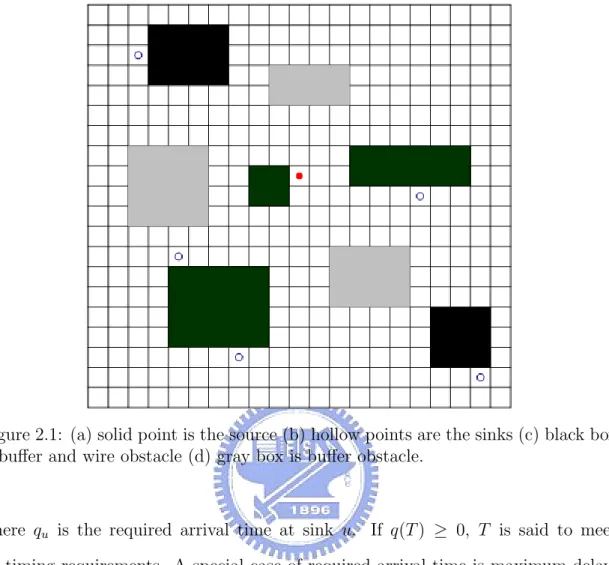
(16) Figure 2.1: (a) solid point is the source (b) hollow points are the sinks (c) black box is buffer and wire obstacle (d) gray box is buffer obstacle.. where qu is the required arrival time at sink u. If q(T ) ≥ 0, T is said to meet its timing requirements. A special case of required arrival time is maximum delay: letting qu = 0 for each sink u, the max source-to-sink delay is −q(T ). The goal of our algorithm is to construct a routing tree with buffer insertion in the presence of wire and buffer obstacles so as to minimize the Elmore delay from source to sink. In our works, we consider two kinds of objectives. Both the objectives are given here: Problem Formulation 1: Given a routing grid G=(V,E), a buffer library B, a source node s ∈ V , k sink nodes t1 , t2 , . . . , tk ∈ V of net and blockages. Find a buffered routing tree T rooted at s and leafed at t1 , t2 , . . . , tk , such that the maximal delay is minimal. Problem Formulation 2: Given a routing grid G=(V,E), a buffer library B,. 5.

(17) a source node s ∈ V , k sink nodes t1 , t2 , . . . , tk ∈ V of net and blockages. Find a buffered routing tree T rooted at s and leafed at t1 , t2 , . . . , tk , such that the slack1 is maximum. The difference between formulation 1 and formulation 2 is the measurement of delay. The former is in top down fashion, the latter is in bottom up fashion. The problem instance is illustrated in Figure 2.1. Two kinds of blockages are considered [21]. The gray box represents routing obstacle region where buffer insertion is infeasible. The black box represents routing obstacle regions where both wire placement and buffer insertion are infeasible.. 2.2. Performance-Driven Interconnect Tree Synthesis. To achieve a minimum-area layout, circuit interconnections should in general be realized with minimal wire length. The objective of minimal wire length corresponds to the Steiner minimal tree (SMT) problem [12]. To achieve a high performance design, only minimizing the total wire length may cause the poor signal delay from source to sink. Thus the problem of performance-driven tree construction arises. An early work of Cohnoon and Randall [5] is notable for its prescient insights. For any given signal net, [5] proposed the construction of a “maximum performance tree” corresponding to “a shortest path . . . with minimum total length”, and noted that such a tree seems difficult to construct. Next, we present the heuristics of performance-driven tree construction with geometric approaches.. 2.2.1. Geometric Approaches to Delay Minimization. C. J. Alpert et al. [4] combined minimum tree cost and minimum tree radius objectives. Tree cost means the total wire length of the tree. Tree radius means the 1. Slack is defined as the difference between the required arrival time and the actual arrival time.. 6.

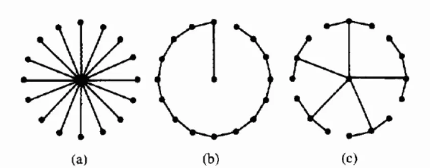
(18) Figure 2.2: Three interconnection trees for the same signal net with s0 at the center: (a) the shortest paths tree Ts ; (b) the minimum spanning tree TM ; (c) a “tradeoff” between the two constructions. From [4].. longest path from source to all sinks, corresponding to the maximum delay of the tree. Consider a two-terminals net, the optimal delay path is the shortest path from source to sink. If all sinks connect to the source with shortest path, the total wire length might be greater than the wire length of the minimum spanning tree. On the contrary, minimum spanning tree has minimal wire length but tree radius is greater than shortest path tree. Figure 2.2 demonstrates the tradeoff in area and delay (radius). [4] presented a straightforward approach to construct the performance driven tree based on Prim’s minimum spanning tree (MST) and Dijkstra’s shortest path tree (SPT), we called it PD. Prim’s algorithm begins initially with the tree consisting only of source s. The algorithm iteratively adds edge eij and sink si to T, where si and sj are chosen to minimize dij s.t. sj ∈ T, si ∈ S − T.. (2.1). Dijkstra’s algorithm also begins with the tree consisting only of source s. The algorithm iteratively adds edge eij and sink si to T, where si and sj are chosen to minimize lj + dij s.t. sj ∈ T, si ∈ S − T. (2.2). The similarity between (2.1) and (2.2) forms the basis of PD , which iteratively. 7.

(19) Figure 2.3: Sample executions for PD for an 8-sink instance in the Euclidean plane [4]. The edge labels give the order in which the algorithms add the edges into the tree. (a) with c= 13 (radius 15.91, cost=26.34) (b)with c= 23 (radius 10.32, cost=29.69).. adds edge eij and sink si to T, where si and sj are chosen to minimize (c · lj ) + dij s.t. sj ∈ T, si ∈ S − T. (2.3). for some choice of c, 0 ≤ c ≤ 1. When c=0, PD is identical to Prim’s algorithm and constructs trees with minimum cost. As c increases, PD constructs a tree with higher cost but lower radius, and when c=1 PD is identical to Dijkstra’s algorithm. Sample executions of PD for c= 13 and c= 23 is shown in Figure 2.3. The results show that the tree radius conflicts with the tree cost. Rectilinear Steiner Arborescence (RSA) algorithm sweeps the weakness of PD. This algorithm proposed in [7, 1] can further reduce the tree cost without increasing the tree radius by means of extra Steiner points. As illustrated in Figure 2.4, the overlapping edges are eliminated by extra Steiner points. The tree structure from RSA is good for wire capacitance reduction, and has the better tree radius than PD. In our works, we will construct the performance driven tree on the basis of the idea, “maximum performance tree” corresponding to “a shortest path . . . with 8.

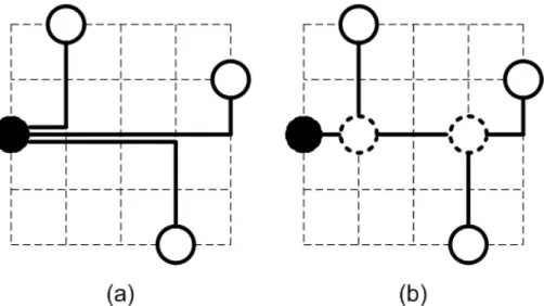
(20) Figure 2.4: RSA to add extra Steiner points. (a) Tree cost=13, overlapped length=4 (b) Tree cost=9, overlapped length=0. Solid circle is the source, other circles are sinks.. minimum total length”, brought by Cohnoon and Randall [5].. 2.3. Van Ginneken’s Algorithm. In this section, we will explain the procedure of buffer insertion, which executes in bottom-up fashion [20]. Consider a RC network in Figure 2.5, each sink has a specified required time and a load capacitance. Using the Elmore delay model, the delay from source to sinks can be calculated recursively. A subtree rooted at k is modeled by a set of tuple (Tk , Lk ). The definition of duple (Tk , Lk ) is : 1. Tk is the required time when the root is driven by a buffer of zero impedance. 2. Lk is the load of the sub-tree. Because the solutions of internal nodes are not unique except for the leaves, we should consider all possible combination of children solutions. For instance, if root k has two children, m and n, m has two solutions (400,10), (200,8), n has one solution (300,12). After merging the solutions of m and n , root gets two solutions (300,22) 9.

(21) Figure 2.5: (a) The physical routing topology; (b) the RC network of (a).. and (200,20). The formulas for evaluating the solution set of root is listed below: Tk(ith) =. min. ¡. all child j. Lk(ith) =. Tj − rlLj − 1/2rclj2. X. ¢ (ith). (Lj + rlj )(ith). (2.4). (2.5). all child j. where the subscript ith means the ith possible combination of children solution. The total solution size of node k after combining all children solutions is Y. (solution size of the jth child). all children. We then add the buffer at the node k, the new (Tk , Lk )buf is evaluated by Tk buf = Tk − Dbuf − Rbuf Lk. (2.6). Lk buf = Cbuf. (2.7). 10.

(22) The whole buffer insertion steps are shown in Figure 2.6. The function “Bottom up” first check whether root is a leaf node (Line 1-3), if not the function is called recursively to compute the solution for all children (Line 5-6). Then generate all the possible solutions after combining children solutions (Line 8-10). Finally, evaluate the solution when root is driven by a newly added buffer (Line 12-14). Bottom up(root) 1 if root is leaf 2 root → T = Tsink 3 root → L = Lsink 4 else 5 for each child i 6 bottom up(root → childi ) 7 // ( Evaluate the root solution according to the children solution ) 8 for all possible combination of children solutions ¢ ¡ 9 root → T(ith) = minall child j Tj − rlj Lj − 1/2rclj2 (ith) P 10 root → L(ith) = all child j (Lj + clj )(ith) 11 // ( Evaluate the root solution after adding buffer) 12 for all solutions after connecting children to root ¡ ¢ ¡ ¢ 13 root → Tbuf (ith) = root → T(ith) − Dbuf − Rbuf root → L(ith) 14 root → Lbuf (ith) = Cbuf Figure 2.6: Dynamic Programming Algorithm for Buffer Insertion [20].. 11.

(23) Chapter 3 Buffered Interconnect Tree Construction with Simultaneous Topology Generation and Buffer Insertion In this chapter, we focus on the buffered interconnect tree construction with simultaneous topology generation and buffer insertion. The main drawback of concurrent approaches in tree construction is that it is time consuming. S. Dechu et al. [9] presented a stochastic search algorithm to efficiently construct a routing tree with simultaneous buffer insertion and wire sizing in presence of wire and buffer obstacles. They used simulated annealing algorithm to randomly adjust the buffered tree. Through the stochastic search algorithm, the solution space for buffered tree topology are quite large. It raises the probability to achieve the minimum tree delay. Nevertheless, uncertainty is this approach’s shortcoming. We desire to diminish the uncertainty of the stochastic approach by hierarchal decomposition. This intention of hierarchy decomposition is similar to the Prim-Dijkstra tradeoff algorithm as mentioned before [4]: reducing the redundant wirelength. The hierarchical tree that we build is two level structures. The structure also was used in [3]. We divide all sinks into several groups. Group is composed of closest sinks, and assigns the nearest sink to source as the root of group. Then construct the 12.

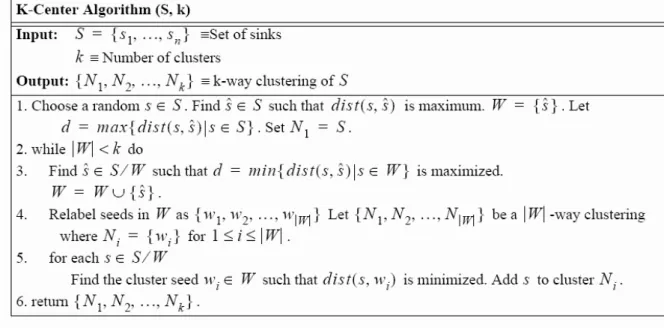
(24) Figure 3.1: Two level routing: clustering all sinks first, and then construct the lowlevel buffered tree over each group. The top-level buffered tree is merged with the low-level buffered trees finally.. low-level buffered tree for each of these groups by the simulated annealing method [9]. Finally, the top-level buffered tree is merged with the low-level subtrees to yield a solution for the entire net. In the following section, we introduce the clustering algorithm, and the simulated annealing algorithm for buffered tree construction.. 3.1. Clustering. For clustering sinks, we adopt the K-center heuristic [3] which attempts to minimize the maximum radius (distance to cluster center) over all clusters. K-center iteratively identifies points that are furthest away; which we called the cluster seed. The complete description of K-center algorithm is shown in Figure 3.2. Step 1 pick a random sink s, then identifies the sink ˆs furthest away from s, which will lie on the periphery of the data set. This step identifies ˆs as the first cluster seed, and all seeds are contained in the set W. Steps 2-5 iteratively find |W | -way clustering N until the clusters equal the number we assign. Step 3 identifies the next seed which 13.

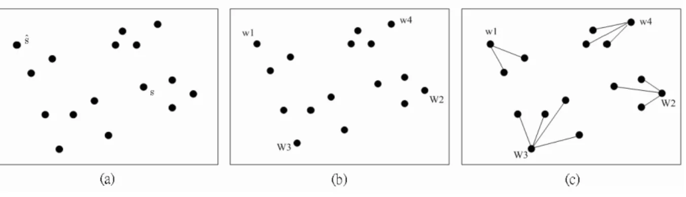
(25) Figure 3.2: K-Center clustering algorithm over a set of sinks S.. is the furthest away from already identified seeds. Steps 4-5 form a clustering by assigning each sink to the cluster corresponding to its closest seed. Step 6 returns the final clustering. Figure 3.3 illustrates an example of the K-center algorithm applied to a 2dimensional data set with 16 points, where k=4. In (a), a random point s is chosen and then the point sˆ which is furthest from s is identified. In (b), this is relabeled as w1, a cluster seed. The order that the four seeds identified are indicated by the subscripts: w2 is furthest from w1, w3 is furthest from both w1 and w2, and w4 is the furthest point from w1,w2 and w3. In (c), each point is mapped to its closest seed, revealing four clusters.. 3.2. Simulated Annealing Method For Buffered Tree Construction. The main idea of simulated annealing method is to use a reconfigurable buffered tree to find the buffered tree with minimal delay. A node of a tree indicates a feasible 14.

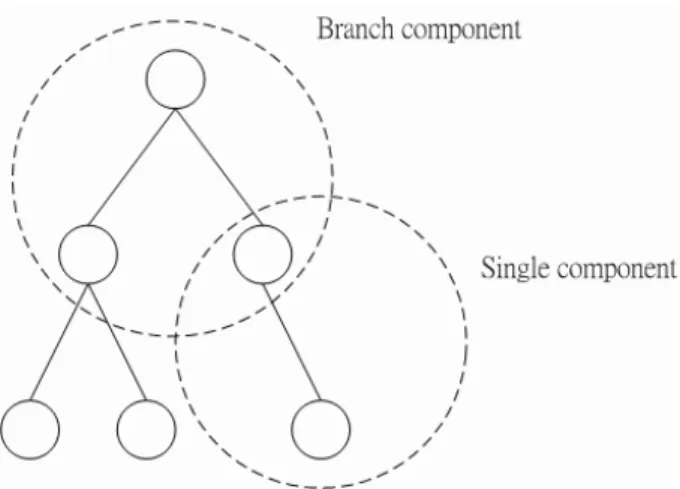
(26) Figure 3.3: 16 points example illustrating the K-center algorithm.. Figure 3.4: The tree has 7 nodes and 6 edges corresponds to (b) in routing graph.. buffer location on the physical plane, and an edge corresponds to the path with the minimal delay for its two terminals. Figure 3.4 demonstrates how a tree represents a real routing. The technique is called Embedding by [10].. 3.2.1. Decomposition of Routing Tree. One observation for the routing tree structure is that the tree can be seen as the set of single component and branch component (Figure 3.5). When a node has two or more children , we identify the node and its children as a branch component. When 15.

(27) Figure 3.5: Routing tree decomposition. A tree is composed of two kinds of components: single component and branch component.. a node has only one child, we identify the node and its child as a single component.. 3.2.2. Component Construction. To evaluate the delay and wirelength of buffered tree, the delay and wirelength of each component should be pre-computed. To obtain the optimal delay for each component, we construct the following tables: 1. Length & Delay Table for Wire Path: Compute the shortest path length dist(a,b) and the delay delay(a,b) for two nodes, where a and b are the locations of two nodes. Note that no buffer is placed among the path from a to b. 2. Length & Delay Table for Segment Wire path: Compute the table for optimal delay of segment wire path Delay(a,b) and table of the length Length(a,b). We use the dynamic programming technique to construct the tables. Then we can find the edge cost in the tables, Length(a,b) and Delay(a,b), to evaluate the cost of each component. 16.

(28) Figure 3.6: Transformation of non-binary tree to binary tree.. 3.2.3. Routing Tree Perturbation. We use a binary tree to represent a routing tree. In addition, to overcome the restriction of binary tree for at most two fanout, the dummy node is defined. Figure 3.6 shows the transformation while a node has high fanout(greater than 2). We only permit the dummy node being right children of a node, which can avoid redundant binary tree. The initial tree is a complete binary tree, and all the leaves are sinks. To reconfigure the tree, four moves are defined to change the tree topology. In annealing process, we randomly apply these moves and expect to minimize cost of the tree by serial moves. The cost function is defined as Tree cost = α× delay + β× wirelength + γ× number of buffers. The four moves are described below: 1. Move 1 - Component Driver Position Change: In simulated annealing, we change the positions of component drivers of single component and branch component. We randomly select one buffer node among 8 adjacent nodes and change the position of the component driver to that position. 2. Move 2 - Swapping of Sinks: This is a topology changing move. In this move, 17.

(29) Figure 3.7: Rotation operations.. we randomly select two sinks driven by two different parents and swap their parents. 3. Move 3 - Conversion between Dummy and Real Nodes: We select a buffer node randomly among the tree and make that node dummy if it is real. On the other hand, make the node real if it is dummy. 4. Move 4 - Rotation: This is also topology changing move. In this move, we have two types of rotation, one is left rotation and other is right rotation. Figure 3.7 shows these two operations. Using these operations we can get all binary trees that can be constructed with the given terminals. When we are making right or left rotations, if a node is violating the restriction, the only right child of a parent can be dummy, we change that dummy node to real node and then make the rotation.. 3.3. Summary. In this chapter, we first use the K-center heuristic to cluster all sinks into several groups. We use the two level hierarchy to save the wirelength and obtain lower load. Then we apply the fast simulated annealing method to construct routing for each group. The two level hierarchy use the spirit of divide and conquer, it runs faster 18.

(30) than flat simulated annealing method and has less wirelength. However it also has a disadvantages, it may cause a longer tree radius in some cases.. 19.

(31) Chapter 4 Buffered Interconnect Tree Construction via Two-Stage Optimization 4.1 4.1.1. Performance-Driven Tree Construction Routing Grid Graph. Before constructing the performance driven tree, we should first build the routing grid graph. Here we overload two concepts for a graph edge and a “physical” (i.e., embedded in the plane) edge, when we speak of “connecting a point a to a point b”. Implicitly, we assume that one possible physical shortest path exist to connect a and b. For instance, in Figure 4.1, the graph edge eaÃc corresponds to the physical path a Ã b Ã c or a Ã d Ã c. The grid graph can represent the environment of physical plane and contain all connections of each point. Taking the efficiency into consideration, we only select some points in the plane to construct the grid graph. We sketch the cross lines on the source and sinks and draw the lines close to the blockage edges, the intersections of these lines are the candidates that we select to construct the grid graph (Figure 4.2). The grid graph contains the following data:. 20.

(32) Figure 4.1: Embedding example: (a) grid graph corresponds to (b) physical plane. In (a), the edge cost equals the length of the shortest path of the endpoints.. • Source: Coordinate (x,y), output resistance (unit:ohm). • Sinks: Coordinate (x,y), required time (unit:ps) and load capacitance (unit:pF). • Blockages: Blockages type and location (x1 , y1 , x2 , y2 ), where (x1 , y1 ) is bottom-left point and (x2 , y2 ) is top-right point. We have two blockage types. Buffer blockages do not permit allocating buffer. Wire blockages do not permit allocating buffer and wire. • Table of the shortest path length: Dist(a, b) is the shortest path length between a and b. Here, we use the Lee’s algorithm to compute the shortest path length for each path.. 4.1.2. Iterated Dominance Algorithm (IDOM) [1]. This section is the procedure of performance driven tree construction, IDOM. IDOM constructs a shortest path tree with minimum wire length. The spirit of IDOM is to remove the overlapping paths in shortest path tree to yield the greatest possible wirelength savings while still maintaining the shortest path property. We define the dominance property to judge whether a point is a candidate steiner point where is potentially good for wirelength minimization. 21.

(33) Figure 4.2: Grid graph: The dotted lines are underlying grid lines and the thick lines are lines for routing. Dark point is the source and gray point are the sinks. Dark boxes are wire blockages and gray boxes are buffer blockages.. Dominance Property: Given a weighted graph G=(V,E), and nodes n0 ,p,s ∈ V , we say that p dominates s if minpathG (n0 ,p)=minpathG (n0 ,s)+minpathG (s,p) In other words, a node p dominates a node s if there exists a shortest path from the source to p that also passes through s. Figure 4.3(a) illustrates the condition of dominance. When one node is dominated by two or more nodes, we can reduce the total wire length by changing the topology , for example in Figure 4.3(b). In this case, the original wirelength equals 19, and the improved wirelength equals 15 (get 21% of wirelength reduction). The notation, DOM(G,N), represents a tree, where G is the grid graph and 22.

(34) Figure 4.3: (a) Illustration of Dominance property and (b) change the tree topology to minimize wirelength according to the Dominance property.. N is the set of nodes in the tree. Consequently, we define the tree cost saving as S ∆DOM(G,N’,s)=cost(DOM(G,N’)-cost(DOM(G,(N’ t))), where N’ is the union of source, sinks and the set of Steiner candidate S, t is the new added Steiner candidate. IDOM starts with connecting sinks to source directly and an empty set S of Steiner candidate. Then, iteratively find the Steiner candidate t ∈ V-(N S) which maximizes ∆DOM(G, N’, t) > 0, and put t into the set of Steiner candidate, S. The method, IDOM, is formally described in Figure 4.4. We use an example in Figure 4.5 to demonstrate how the IDOM greedily adds Steiner points to construct a solution. IDOM can reduce 37.5% of total wirelength from this instance.. 4.2 4.2.1. Buffer Insertion Efficient Buffer Insertion. Recall the method of delay calculation and buffer insertion in Section 2.2, the solution set of a node is evaluated by combining solution set of children. However, some of the solutions can be pruned according to the property: F or (T, L) , (T 0 , L0 ) ∈ S , if L0 ≥ L and T 0 < T then (T 0 , L0 ) is suboptimal. 23.

(35) The Iterated Dominance (IDOM) Heuristic Input: A weight graph G=(V,E), a net N ⊆ V Output: A low-cost arborescence T’=(V’,E’) spanning N, where N ⊆ V’ ⊆ V and E’ ⊆ E S=∅ Do Forever S S T={t ∈ V-(N S)} | ∆ DOM(G,N,S S {t} > 0}) IF T=∅ Then Return DOM(G,N S) S FindSt ∈ T with maximum ∆ DOM(G,N,S {t}) S=S {t} Figure 4.4: The Iterated Dominance (IDOM) algorithm.. Figure 4.5: Execution example of the IDOM algorithm: (a) Initial DOM solution, having cost 24; (b) Steiner candidate s1 produces a savings of ∆DOM=8, which reduces the overall tree cost to 17; (c) Steiner candidate s2 produces a savings of ∆DOM=1, which reduces the overall tree cost to 16; (d) Final solution, the last Steiner candidate reduces the tree cost to 15.. 24.

(36) Algorithm Merge Solution() S=∅ For i = 1 . . . n, n is the number of children Ptr(i) = children(i)· front Do Forever Until one of Ptr is null Temp = S Merge ALL Ptr() S = S Temp Find the critical Ptr(i), and then Ptr(i) = Ptr(i)·next Figure 4.6: Algorithm for merging the children solution sets at branch.. It is clear that a larger load could only worsen delay of ancestor components. In other words, we always prefer smaller load and larger required time. Supposing the sets are arranged in increasing order of load will lead the following property: Any load required time set S in increasing order of load may be replaced by S 0 ⊆ S where S 0 is strictly increasing in required time. For maintaining the above property, we use the linked list to store the solution. At the branch point, we can efficiently prune the redundant solutions by a merge technique. The merging procedure is shown in Figure 4.6. At each step we merge the solutions selected in different solution list. Then we replace the critical one among the selected solutions with the next solution. The merging process is illustrated in Fig 4.7. Having the pruning rule, we should modify the algorithm in Section 2.2. The complete algorithm is listed in Figure 4.8.. 4.2.2. Buffered Tree Transformation. Due to the recursion of buffer insertion algorithm, it runs from the leaves to the root. The tree structure we construct will produce the following condition: sink 25.

(37) Figure 4.7: Example of merge operation. The two columns on the left are the solution sets being merged; pairs of solution combined are surrounded by circle. The resulting set of solutions appears on the right.. Algorithm Bottom Up(root) if root is leaf evaluate the sink solution else for i = 1 . . ., n is the number of children Bottom Up(children(i)) if root is not branch evaluate the sorted solution for root else evaluate all sorted solution of children Merge Solution() evaluate the optimal buffer solution Figure 4.8: Dynamic Programming Algorithm for Buffer Insertion With Pruning [15, 20].. 26.

(38) nodes may be the parents of other nodes. To easily execute the buffer insertion algorithm, we do not permit the sinks having any children. We slightly change the tree structure, and force all sinks to the leaves of the tree by additional pseudo nodes. An example is illustrated in Fig 4.9. In this example, the sink, t1 , has one child s1 . We then generate a pseudo node, s2 , at the same position with t1 . We complete the transformation by producing the edges, es2!s1 , es2!t1 and eroot!s2 , and breaking the edges, eroot!t1 and et1!s2 . Next, we consider the different conditions of buffer connection at the branch point and further change the tree topology to handle all possible conditions. In Figure 4.10, (a) is the topology we considered, it might have buffer conditions, (b), (c), (d), (e), (f), (g) and (h). Since the optimal solution can be computed by the buffer insertion algorithm, we can transform the tree with the same technique to the final structure as (i). Through this simple transform action, we can obtain the solutions better than the solutions without considering the different buffer connection at branch point. This is because now we can take all possible conditions of buffer connection into account, not only (b) and (c). We called this transform action as “decouple function” in our platform.. Figure 4.9: Illustration of tree transformation.. 27.

(39) Figure 4.10: (a) Consider all buffer combinations at candidate point C. (b) Buffer is not inserted at C. (c) One buffer at C drives t1 and t2. (d) One buffer at C drives only t1. (e) One buffer at C drives only t2. (f) Two buffers at C drive t1 and t2 respectively. (g)&(h) Two buffers are inserted at C, and one buffer decouple t1 or t2. (i) Candidate point C transform to three pseudo point to handle all buffer combinations.. 28.

(40) 4.3. Summary. The entire flow of our two-stage buffered tree construction algorithm follows these steps: 1. Construct the grid graph 2. Construct the performance-driven routing tree based on IDOM algorithm. 3. Transform the tree structure (option: consideration for all possible conditions of buffer connection at branch point). 4. Execute the buffer insertion algorithm for the tree.. 29.

(41) Chapter 5 Experimental Results We have implemented two approaches for buffered interconnect tree construction in C++ and tested it on Pentium 4 PC 2.4GHz with 512MB memory, one is two-level hierarchical simulated annealing algorithm and the other is two-stage buffered tree algorithm. To show the effectiveness of our approaches, we compare the results with the fast flat simulated annealing algorithm [9]. We use the same technology parameters given in [19], as shown in Table 5.1. Our chip size is 17 × 17 mm2 with horizontal and vertical grid lines spaced at 0.5mm distance from each other. Table 5.1: Technology Parameters. Wire Capacitance Wire Resistance Buffer Output Resistance Buffer Input Capacitance Buffer Intrinsic Delay. 0.108(pF/µm) 0.076 (Ω/µm) 180 (Ω) 0.024 (pF) 36.4 (ps). Table 5.2 and 5.3 show the comparison between these four methods. In Table 5.2 and 5.3 , we use a single buffer type and two buffer types respectively. We now examine the efficiency and performance of these algorithms. For execution time, the simulated annealing algorithm has long execution time, but the two-stage algorithm remains the same execution time. This is because the run time of performance 30.

(42) Table 5.2: Performance comparison (Buffer Types = 1, Blockages = 11) between the approaches in [9] and our approaches. Our two-stage approach has better delay and wirelength in comparison with SA algorithm.. buf. delay. WL. (ps). (mm). 1292. 77. 20. NET11. 976. 78.5. 21. NET18. 1239. 124. 29. NET23. 1319. 141. 35. NET25. 1084. 154. 45. name. NET8. Two-Stage (Decouple Off). Two-Level SA. Flat SA. DATA. buf. CPU. delay. WL. (sec). (ps). (mm). 5.88. 1284. 73. 18. 8.0. 955. 74.5. 15. 8.86. 1059. 99. 21. 10.23. 1100. 106. 25. 11.86. 1182. 117.5. 26. Two-Stage (Decouple On) CPU. delay. WL. (sec). (ps). (mm). 20. 0.64. 1249. 65. 21. 0.64. 66.5. 20. 0.73. 859. 66.5. 22. 0.73. 94.5. 30. 1.15. 1035. 94.5. 34. 1.15. 1037. 96. 32. 1.54. 992. 96. 35. 1.54. 1055. 97.5. 33. 1.7. 999. 97.5. 37. 1.7. delay. WL. (sec). (ps). (mm). 5.05. 1309. 65. 4.5. 892. 5.67. 1118. 6.69 7.5. buf. driven interconnect tree construction is fixed and the run time of buffer insertion algorithm is very fast. However the simulated annealing algorithm spends long time on lookup table construction and also needs time to search the optimal buffered tree, hence it will use more time when using multiple buffer types. For performance, our two-stage algorithm has better performance in our most experimental cases. The main reason is the performance-driven tree has lower load and tree radius, and the performance is naturally better than the results of simulated annealing algorithm. In addition, if we turn on the decouple function of the two-stage algorithm, we can get more delay reduction. Figure 5.1 and 5.2 are examples for “decouple off” and “decouple on” respectively. We further discuss these two proposed algorithm in details. The two-level hierarchical buffered tree construction is based on simulated annealing algorithm [9]. The simulated annealing algorithm mainly emphasizes that the execution time is less than previous simultaneous approaches [16, 11]. However, we find this approach has a major drawback. Its solution is very uncertain especially when terminal number of net is large. When terminal number of net is large, the wirelength of buffered tree constructed by simulated annealing algorithm appears very long. We believe. 31. buf. CPU. CPU. (sec).

(43) Table 5.3: Buffer Types = 2, Blockages = 11. The 2nd buffer’s parameters: output resistance=90(Ω), input capacitance= 0.048(pF), intrinsic delay=36.4(ps).. 25. 0.73. 94.5. 34. 1.15. 875. 94.5. 36. 1.15. 870. 96. 32. 1.54. 838. 96. 34. 1.54. 880. 97.5. 35. 1.7. 841. 97.5. 36. 1.7. 924. 114. 24. 56.08. 131.5. 28. 55.31. 926 1018. 198. 994. 66.5. 47.95. 104. 127.42. 1135. NET25. 728. 19. 927. 55. NET23. 0.73. 66.5. 17. 58. 141.5. 22. 753. 74.5. 195. 1104. 0.64. 42.86. 796. 173.5. NET18. 23. 20. 100. 24. 65. 65. 36. 80.5. (mm). 1049. (mm). 61.98. 837. NET11. (ps). 0.64. (ps). 1085. (mm). (mm). 1180. CPU. the longer wirelength is the reason why it has bad performance and use a lot of buffers. To improve this disadvantage, we try to use two-level hierarchical method to minimize the wirelength. From our experimental results, the two-level hierarchical method has better wirelength and use less buffers. However it has a little bad delay for some cases, we think the result may be caused by the longer tree radius. To improve the disadvantages of the above algorithms, we propose the method of two-stage buffered tree construction. We believe performance-driven tree construction and buffer insertion can be done independently. We do not need to consider both of them at the same time. If we can construct a interconnect tree which is potentially good for delay and insert buffers for it, we can get a good enough solution. From our experimental results, our two-stage algorithm has better performance than the simultaneous approaches and use less buffer resources and wire resources. The two-stage algorithm is also more efficient than simulated annealing algorithms.. 32. CPU. (sec). (sec). 19. (ps). 1196. 23. (ps). NET8. buf. WL. 41.94. 74. (sec). 53.73. 76. WL. delay. WL. CPU. WL. CPU. delay. buf. delay. buf. delay. buf. name. Two-Stage (Decouple On). Two-Stage (Decouple Off). Two-Level SA. Flat SA. DATA. (sec).

(44) Figure 5.1: The decouple function of Two-Stage-Method turn off. Delay = 1309 (ps), wirelength = 65 (mm), # of buffer = 20.. Figure 5.2: The decouple function of Two-Stage-Method turn on. Delay = 1249 (ps), wirelength = 65 (mm), # of buffer = 21.. 33.

(45) Chapter 6 Conclusion and Future Work Since the interconnect delay becomes more important, we should take it into consideration during chip design. The buffer insertion algorithm can minimize the delay of fixed tree. However, the solution may be limited by the input tree. [9] proposed a fast simulated annealing algorithm which simultaneously constructs the routing tree and performs buffer insertion. But this algorithm suffers from the problem of uncertainty when the terminal number of net is large. We try to solve this problem by clustering. We get wirelength reduction and use less buffer resources. But in some cases, the clustering algorithm may cause worse delay due to longer tree radius. We believe that the routing tree construction and buffer insertion can be independently performed. We propose the two stage algorithm to efficiently construct the buffered tree. First we construct a performance-driven interconnect tree, then apply the buffer insertion algorithm to minimize delay. From the experimental results, our algorithm is more efficient than [9] and can obtain better delay. We draw the conclusion that the two-stage algorithm can use less run time and get better performance than the simultaneous approach by decoupling technique. In future works, we plan to further improve our two-stage algorithm by wire sizing. We can also find another approach to synthesizing a better performance-driven tree.. 34.

(46) Acknowledgment: We thank Dr. Xiaoping Tang and Prof. Chris C. N. Chu for providing their platforms in experimental results comparison.. 35.

(47) Bibliography [1] M. J. Alexander and G. Robins. “New Performance-driven FPGA Routing Algorithms”. IEEE Transactions on Computer-Aided Design of Integrated Circuits and Systems, 15(12):1505–1517, Dec. 1996. [2] C. J. Alpert, A. Devgan, and S.T. Quay. “Buffer Insertion with Adaptive Blockage Avoidance”. IEEE Transactions on Computer-Aided Design of Integrated Circuits and Systems, 18(11):1633–1645, Nov. 1999. [3] C. J. Alpert, G. Gandham, M. Hrkic, J. Hu, A. B. Kahng, B. Liu J. Lillis, S. T. Quay, S. S. Sapatnekar, and A. J. Sullivan. “Buffered Steiner Trees for Difficult Instances”. In Proceedings International Symposium on Physical Design, pages 4–9, 2001. [4] C. J. Alpert, T. C. Hu, J. H. Huang, A. B. Kahng, and D. Karger. “PrimDijkstra Tradeoffs for Improved Performance-driven Routing Tree Design”. IEEE Transactions on Computer-Aided Design of Integrated Circuits and Systems, 14(7):890–896, July 1995. [5] J. P. Cohoon and L. J. Randall. “Critical Net Routing”. In Proceedings IEEE International Conference on Computer Design, pages 174–177, 1991. [6] J. Cong. “Challenges and Opportunities for Design Innovations in Nanometer Technologies”. In Semiconductor Research Corporation Design Sciences Concept Paper, pages 1–15, 1998. 36.

(48) [7] J. Cong, A. B. Kahng, and K.-S. Leung. “Efficient Algorithms for The Minimum Shortest Path Steiner Arborescence Problem with Applications to VLSI Physical Designs”. IEEE Transactions on Computer-Aided Design of Integrated Circuits and Systems, 17(1):24–39, Jan. 1998. [8] J. Cong and X. Yuan. “Routing Tree Construction Under Fixed Buffer Locations”. In Proceedings IEEE/ACM Design Automation Conference, pages 379–384, 2000. [9] S. Dechu, C. Shen, and C. Chu. “An Efficient Routing Tree Construction Algorithm with Buffer Insertion, Wire Sizing and Obstacle Considerations”. IEEE Transactions on Computer-Aided Design of Integrated Circuits and Systems, 24(4):600–608, April 2005. [10] M. Hrkic and J. Lillis. “S-Tree: A Technique for Buffered Routing Tree Synthesis”. In Proceedings IEEE/ACM Design Automation Conference, pages 578– 583, 2002. [11] M. Hrkic and J. Lillis. “Buffer Tree Synthesis with Consideration of Temporal Locality, Sink Polarity Reuirements, Solution Cost and Blockages”. IEEE Transactions on Computer-Aided Design of Integrated Circuits and Systems, 22(4):481–491, April 2003. [12] F. K. Hwang, D. S. Richards, and P. Winter. “The Steiner Tree Problem”. North-Holland Publisher, 1992. [13] S. S. Sapatnekar J. Hu. “Algorithms for Non-Hanan-Based Optimization for VLSI Interconnect under a Higher-Order AWE Model”. IEEE Transactions on Computer-Aided Design of Integrated Circuits and Systems, 49(4):446–458, April 2000.. 37.

(49) [14] M.-H. Lai and D.F. Wong. “Maze Routing with Buffer Insertion and Wiresizing”. IEEE Transactions on Computer-Aided Design of Integrated Circuits and Systems, 21(10):1205–1209, Oct. 2002. [15] J. Lillis, C.-K. Cheng, and T.-T. Lin. “Optimal Wire Sizing and Buffer Insertion for Low Power and a Generalized Delay Model”. IEEE Transactions on Computer-Aided Design of Integrated Circuits and Systems, 31(3):437–447, March 1996. [16] J. Lillis, C.-K. Cheng, T.-T Lin, and C.-Y. Ho. “New Performance Driven Routing Techniques with Explicit Area/Delay Tradeoff and Simultaneous Wire Sizing”. In Proceedings IEEE/ACM Design Automation Conference, pages 395– 400, 1996. [17] T. Okamoto and J. Cong. “Buffered Steiner Tree Construction with Wire Sizing for Interconnect Layout Optimization”. In Proceedings IEEE/ACM International Conference on Computer-Aided Design, pages 44–49, 1996. [18] R. R. Rao, D. Blaauw, D. Sylvester, C. J. Alpert, and S. Nassif. “An Efficient Surface-Based Low-Power Buffer Insertion Algorithm”. In Proceedings International Symposium on Physical Design, pages 86–93, 2005. [19] X. Tang, R. Tian, H. Xiang, and D. F. Wong. “A New Algorithm for Routing Tree Construction with Buffer Insertion and Wire Sizing under Obstacle Constraints”. In Proceedings IEEE/ACM International Conference on ComputerAided Design, pages 49–56, 2001. [20] L. P. P. P. van Ginneken. “Buffer Placement in Distributed RC-tree Network for Minimal Elmore Delay”. In Proceedings Internationl Symposium on Circuits and Systems, pages 865–868, 1990.. 38.

(50) [21] H. Zhou, D.F. Wong, I.-M. Liu, and A. Aziz. “Simultaneous Routing and Buffer Insertion with Restrictions on Buffer Locations”. IEEE Transactions on Computer-Aided Design of Integrated Circuits and Systems, 19(7):819–824, July 2000.. 39.

(51) 作者簡歷游宗達，民國七十年九月出生於花蓮縣。民國九十二年六月畢業於國立交通大學電子工程學系，並於同年九月進入國立交通大學電子研究所就讀，從事 VLSI 實體設計方面相關研究。民國九十四年六月取得碩士學位，碩士論文題目為『考慮障礙物繞線及緩衝器插入之方法研究』。.

(52)