Effective Learning Curve Model and Activate Media Learning Algorithm for Improving Learning Efficiency

全文

(1)Int. Computer Symposium, Dec. 15-17, 2004, Taipei, Taiwan.. Effective Learning Curve Model and Activate Media Learning Algorithm for Improving Learning Efficiency. Shih-Jung Peng, Pi-Feng Liang, and Deng-Jyi Chen psjcpl@thit.edu.tw, pfliang@csie.nctu.edu.tw, and djchen@csie.nctu.edu.tw Institute of Computer Science and Information Engineering National Chiao-Tung University HsinChu, Taiwan 300, ROC. Abstract-In this world, technology developments. world. The things people deal with have become. are speeding. How to learn desired knowledge. more and more complex. Many ten years ago, for the. efficiently has become a complicated problem. In this. research of building airplane, Wright [1] had used. paper, we introduced some learning phenomenon. math methods to create learning curve function and. about people with learning curve and proposed an. develop first thesis about learning curve. From that. Effective Learning Curve Model to emulate this. time, learning methods have been discussed for. phenomenon. Using proposed learning function. distinct application plan and different models also. model, we can understand people’s learning behavior. have been produced. If we set horizontal axis. and know every people has different learning. indicates learning time period on courses, while the. functions on distinct courses. Different course. vertical axis indicates learning efficiency, we call this. learning sequence will cause distinct learning. Figure as learning curve. People’s learning curves are. efficiency. In this view, we proposed Max Learning. different on learning distinct knowledge and will be. Slope First Algorithm (MLSFA) to give people some. changed because of many reasons such as difficulty. suggestions about course learning sequence. This. of. algorithm can help us to understand how much time. background of learners, and some other reasons.. we have to spend on each course in order to get better. There are typical people’s different learning curves. learning efficiency under time limitation. Finally, we. describe as follow, and shown in Figure 1.. make. a. Negative Accelerating Curve. some. learning. example. and. compare. works,. learning. motivation,. simulation results with other learning algorithm.. b. Positive Accelerating Curve. From simulation result, we can see that our MLSFA. c. S Accelerating Curve. algorithm has better learning efficiency than other. d. Linear Accelerating Curve. methods.. knowledge. If there are some courses we prepare to learn, we. Keywords: e-learning, efficient learning algorithm,. can make courses relations into a learning graph as. learning function, learning model, learning efficiency. shown in Figure 2. In this Figure, nodes represent course name and arrows mean course learning. 1. Introduction. sequence, for example, people can not learn course C. Technology development progresses rapidly in the. till course A has passed or the learning efficiency will. 1 1097.

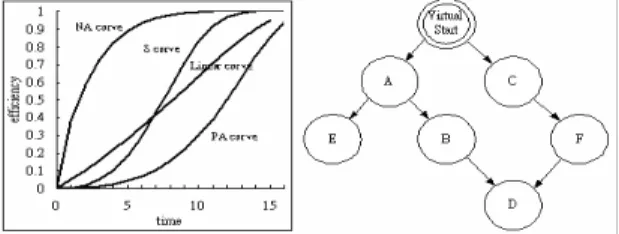
(2) Int. Computer Symposium, Dec. 15-17, 2004, Taipei, Taiwan.. decrease, we set this decreasing parameter ∂. Of. 2. Related work. course, maybe there are some courses independent to. Learning curve can be described in distinct math. others, such as course A and course B. That means. equation for different learning characteristic. Five. we can start learning from either course A or course. commonly used learning curve are described In. B. For this reason, we use ‘virtual start node’ as the. Yelle[2], and are introduced as following:. beginning of learning graph.. a. Log-linear model [1],, f(x) = a1 x -b b. Standford-B model [3], f(x) = a1 (x+B) -b) c. S Curve Model [4], f(x) = a1 ( M + (1-M) (x+B) -b) d. Time Constant Model [6], Y(t)=Yc + Yf (1-e -t/ζ ) All the Learning model in Yelle[2] are suitable for special condition, but can’t cover all learning behavior we have introduced before, and will be. Fig. 1 Typical learning curve Fig. 2 Courses learning of people. limited in some learning application. In this paper,. sequence graph. Under this course learning graph, we hope there. we proposed Effective Learning Curve Model try to. are some suggestions to understand how to get the. emulate all learning behavior of people by tuning. maximum learning efficiency by spending minimum. some function parameter. Then we raise Max. time on each course. For this reason, we introduce. Learning Efficiency Slope First Algorithm (MLESFA). new learning function model to emulate people’s. to improve people’s learning efficiency under. learning behavior on each course and propose max. learning group courses, and make some example to. learning slope first algorithm (MLSFA) under score. prove that our MLESFA algorithm has better learning. base and time base conditions to improve group. efficiency.. courses learning efficiency. At the end, we compare simulation results of our proposed MLSFA algorithm. 3. Heuristic Learning Model. with other learning algorithms. The simulation. In this section, we want to find a question can. comparison is shown in Figure 6 and 7. From. emulate all the learning behavior of people, as in. simulation result, we can see that our algorithm has. Figure 1. At first, we choose 1-e-at as our base. better simulation result and can improve learner’s. function. We all know 1-e-at =1, when t→∞, and. group courses learning efficiency.. 1-e-at =1, if t→0. From the characteristic of exponential. The remainder of this paper is organized as. function, we can see if parameter ｀a＇ changed. follows. The section ІІ, we introduce some related. decreasingly or increasingly between 0 to ∞, and time. work and compare them with our proposed methods.. increasing at the same time, it will produced some. In section ІІІ, we proposed Heuristic learning model. behavior curves like in Figure 1. Under experimentally. to emulate people learning curve. Algorithms for. testing, we take η ( t ) = c (1 − exp( − a ( nt ) )) as. improving Learning efficiency are described in. b. 1 − ( nt ). section IV. The simulation results and comparisons. our learning function model, in that, t is time. are presented in section V. Finally, we provide. sequence, ‘a’ and ‘b’ are function parameter in order. conclusion in section VI.. to emulate. learner’s learning behavior, n is. simulation time slot range, used to 0.01, c is function. 2 1098.

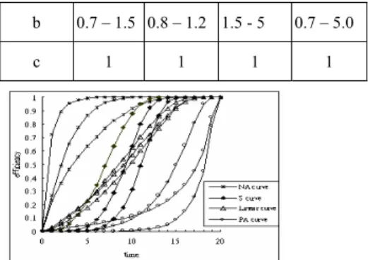
(3) Int. Computer Symposium, Dec. 15-17, 2004, Taipei, Taiwan.. coefficient indicating learning speed of emulated. b. learning function.. c. 0.7 – 1.5 0.8 – 1.2 1.5 - 5 1. 1. 0.7 – 5.0. 1. 1. Using function f = η (t ) , we tune parameter ‘a’, ‘b’ and ‘c’. In the following, we set parameter ‘a’ from 0.1 to 10, ‘b’ from 0.7 to 5 and parameter ‘c’, the speeding coefficient of learning function, to 1. We can get relative function curves shown in Figure 3. Compare these figures, the effects of parameter. Fig. 5 Emulating people’s learning behavior. ‘a’, ’b’ and ‘c’ to function model are shown in Figure 4.. But how can we get the parameter ‘a’, ‘b’ and ‘c’ of each user? We can collect and store much database about the relations of learning efficiency with learner’s personality such as knowledge background, learning attitude, course difficulty, etc. Before. a. ‘a’ = 0.1 to 10, ‘b’=2, ‘c’=1 b. ‘a’ = 0.1 to 10, ‘b’=5, ‘c’=1. learning, we can make some pre-testing to predict. Fig. 3 Emulating learning curve. suitable parameter ‘a’, ‘b’ and ‘c’ of each course respectively in order to get proper learning function to emulate learner’s learning behavior. Under learning group courses, there are some learning sequence relations between courses. So, if we want to. a. curve effect of parameter ‘a’ b. curve effect of parameter ‘b’. get the max learning efficiency in some condition,. Fig. 4 Effects of learning function parameter. the model can be formulated as follow.. From Figure 3, if we want to make a emulation of. Max (. learner’s learning curve, we can only set the range of parameter ‘a’ between 0.1 to 10 , parameter ‘b’. Where,. m. n. i =1. j =1. ∑ ∑W. i. d η i ( t ij ) ) dt. ∗. m: courses number. between o.7 to 5 and c=1. If we want the emulation. n: time slots of studying. curves more precisely, we can just tune parameter ‘c’. Wi: weights of course i. from 0.8 to 2.0. From experiments, effects of. η i (t ) : learning function on course i. parameter ‘a’ on learning function are shown in. d η i ( t ij ) / dt : learning efficiency of. Figure 4.a, effects of parameter ‘b’ are in Figure 4.b respectively. Therefore, we can emulate some different. learning. behavior. curves. spending ∆ time j on course i Subject to. tij≧0, T≧0,. under. combinations of parameter ‘a’, ‘b’ and ‘c’ between. Wi≧0,. different range, as described in Table 1, and the. d η i ( t ij ). Figure 5.. dt. Table 1 Learning behavior under parameter ‘a’, ‘b’, ‘c’. a. 2.0– 10. 0.8 – 1.2 2.0 - 10. In. 0.1 – 0.5. i =1. j =1. i. d η i ( t ij ). i =1. j =1. dt. tj,. =T. =1. ,. n. time. ij. ≥ 0. m. ∑ ∑. parameter PA Curve LA Curve SA Curve NA Curve. n. m. ∑W i =1. emulating learning behavior curves are shown in. m. ∑∑t. ≤ 100. we. choose. max. 3 1099.

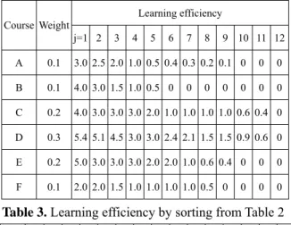
(4) Int. Computer Symposium, Dec. 15-17, 2004, Taipei, Taiwan.. ( w d η 1 ( t j ) , w d η 2 ( t j ) ,.., w d η n ( t j ) ) as first 1 2 n. are two questions we must face to solve. The first. course reading priority.. time on each course for the purpose of getting 60. dt. dt. dt. question is how can we know the minimum spending score to pass the courseware, and the second question. 4. Improving learning efficiency algorithm. is how to obtain maximum course learning efficiency. In this section, our objective is to provide a. in order to get best score under given time limitation.. mathematical analysis in learning courses and to. For these reason, we propose score base algorithm. define behavioral strategies that lead the learning. 1.1 to solve first question, to know the minimum. efficiency to the optimal operating point. Several. spending time on each course for the purpose of. implementation aspects will be briefly discussed in. getting 60 score to pass all the courses, and time base. these works. We assumed there are six courses A, B,. algorithm 1.2 to solve the second question, to get the. C, D, E, F and their weights of each course is. best score under given time limitation.. normalized to be Wi/ΣWi, as in table 2. Using. But because some courses are dependent to each. pre-testing, we can obtain users’ learning curve of. other, if course n-1 has not passed, the learning. each course and get discrete learning efficiency of. efficiency of courses n will be influent. We raise. each unit time by differential course learning. parameter ∂ as this effect, and learning efficiency will. functions Dηi(t)∣t=tj, and multiplying these values. be changed to learning efficiency*(∂^m), in that. with course weight Wi, we get the results in Table 2.. 0≦∂≦1, m is the fail or unlearn courses before. Next, sorting Table 2 on learning efficiency field by. learned course n. To these question, we propose score. descending, we get value as in Table 3.. base algorithm 1.1 to solve first question, to know the. Table 2 Learning efficiency*normalized weight. minimum spending time on each course for the purpose of getting 60 score to pass all the courses,. Learning efficiency Course Weight j=1 2. 3. 4. 5. 6. 7. 8. and time base algorithm 1.2 to solve the second. 9 10 11 12. A. 0.1. 3.0 2.5 2.0 1.0 0.5 0.4 0.3 0.2 0.1 0. 0. 0. question, to get the best score under given time. B. 0.1. 4.0 3.0 1.5 1.0 0.5 0. 0. 0. limitation. At first, we made a course learning. C. 0.2. 4.0 3.0 3.0 3.0 2.0 1.0 1.0 1.0 1.0 0.6 0.4 0. sequence choosing principle, such that,. D. 0.3. 5.4 5.1 4.5 3.0 3.0 2.4 2.1 1.5 1.5 0.9 0.6 0. a.. high level learning course first. E. 0.2. 5.0 3.0 3.0 3.0 2.0 2.0 1.0 0.6 0.4 0. 0. 0. b.. high course weight first with the same level. F. 0.1. 2.0 2.0 1.5 1.0 1.0 1.0 1.0 0.5 0. 0. 0. c.. effecting more learning courses first. d.. learning from left to right. 0. 0. 0. 0. 0. Table 3. Learning efficiency by sorting from Table 2 Time j=1 2. 3. 4. 5. 6. 7. 8. 9 10 11 12 13 14 15. LS. d1 d2 e1 d3 c1 b1 a1 b2 c2 c3 c4 d4 d5 e2 e3. US. 5.4 5.1 5.0 4.5 4.0 4.0 3.0 3.0 3.0 3.0 3.0 3.0 3.0 3.0 3.0. Algorithm 1.1 Score base 1. To do the same step 0 to 4 as in algorithm 1.1. 2. Using course learning sequence choosing principle, we record course learning sequence in array CS, and relative course weight in CW.. .. etc. In the following discussion, first, we have made. 3. Get courses number cn. the assumption that some courses are dependent to. 4. For i=1 to cn. others, as shown in Figure 7. In this condition, there. 5. Do while (total score (i) < wanted score). 4 1100.

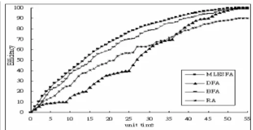
(5) Int. Computer Symposium, Dec. 15-17, 2004, Taipei, Taiwan.. Get max chapter learning efficiency from course. SD=60, SE=70, SF=65, respectively. Therefore if we. i and record obtained score from score Table 2. want to pass all the courses, we must spend at least to. 7.. Record course chapter learning sequence to LS. 21 unit times, and will obtain final score equal to 66. 8.. Increase and record course chapter learning time. with multiplying each course score by course. 6.. 9. End Do. weighting. Another question is that, if we have unit. 10. Next i. time >21, for example 30, what score we can get max?. 11. Print wanted results. First, we use algorithm 1.1 to make all courses pass, and then use algorithm 1.2. We can obtain the time. Algorithm 1.2 Time base. we spend on each course, TA=3, TB=3, TC=5, TD=9,. 1. To do the same step 0 to 4 as in algorithm 1.1.. TE=6, TF=4 and get related scores as follow, SA=75,. 2. Using course learning sequence choosing principle,. SB=85, SC=75, SD=95, SE=90, SF=65. At last, we. we record course learning sequence in array CS,. obtain final score equal to 84. And the course. and relative course weight in CW.. learning sequence suggestion is stored in variable LS.. 3. Get courses number cn. 5. Efficiency comparison. 4. For i=1 to cn. For proving our learning function and algorithms. 5. Do while (total score (i)<60 and total learning. having better learning efficiency, we use learning. time < time limited) Get max chapter learning efficiency from. graph, Figure 6 and Figure 7, as our simulation. course i and record obtained score from score. example. Table 2 is learner’s learning efficiency of. Table 2. each course by differential course learning function. 7.. Record course chapter learning sequence to LS. from discrete data sampling. At the first, we take. 8.. Increase course chapter learning time and record. Figure 6 into consideration that courses are. 6.. 9.. independent, and we compare MLESFA1 simulation. End Do. 10. Next i. result with Depth First algorithm (DFA), Bread First. 11. Do while (total learning time < time limited). algorithm (BFA) and Random algorithm (RA). DFA. 12. Get max learning efficiency course chapter and. learns all chapters of course A by sequence, and then. record obtained score from score Table 3. course B, C, D, E and F. BFA learns chapter 1of. 13.. Record course chapter learning sequence to LS. course A next chapter 1 of course B, C, D, E, and F,. 14.. Increase course chapter learning time and record. after that, learns chapter 2 of course A, B, C,D,E,F. 15. End Do. and will not stop till all chapters have been learned. 16. Print wanted results. completely. RA means random choosing course. From the example of learning graph as in Figure 7, using algorithm 1.1 and 1.2, we can get course learning sequence such as course C, A, E, B, F, and D. If we want to pass all courses, the time we must spend on each course is TA=3, TB=2, TC=4, TD=4, TE=4, TF=4 and each course score we will get is as. chapter to learn. Because of course chapter having its learning sequence, random choosing course chapter to learn will affect chapter learning efficiency, we assume effect parameter η=0.9. The comparison learning efficiency curves are shown in Figure 6 under course learning graph Figure 6.. follow, SA=75, score of course A, SB=70, SC=65,. Next, we think Figure 2 that courses are. 5 1101.

(6) Int. Computer Symposium, Dec. 15-17, 2004, Taipei, Taiwan.. dependent as our simulation graph. The courses learning sequence under choosing course learning sequence principle are course A, C, B, E, F, D of algorithm MLESFA, course A, E, B, D, C, F of algorithm DFA , course A, C, E, B, F, D of algorithm BFA respectively. As to algorithm RA, we get randomly courses learning sequence is course F, B, D,. Fig. 8 Efficiency comparison under courses independence.. C, E, A. Because courses are dependent, if parent course haven’t passed, and we insist on learning following courses, the course learning efficiency will be affected. This effect will bigger than courses dependent and we assumed this effect parameter η =0.8. If learning course have m parent courses not. Fig. 9 Efficiency comparison under courses dependence.. passed, the effect parameter will be changed to η^m. The comparison learning efficiency curves are shown. Reference. in Figure 7 under condition Figure 2. From above. [1] Wright, P.T, “Factors Affecting the Cost of. discussion, we can see our algorithm has better. Airplanes,” Journal of Aeronautical Sciences,. learning efficiency result both in Figure 6 under. Vol.3, No.4, 1936, pp.122-128.. Figure 6 of courses independence, and in Figure 7. [2] Yelle, L. E., 1979, “The learning curve: History. under Figure 2 of courses dependence.. Review and Comprehensive Survey,” Decision Sciences, Vol.10, No.3, pp.302-328 [3] Garg, A. and Milliman, P., “The Aircraft Progress. 6. Conclusion In this paper, we proposed new effective. Curve Modified for Design Changes,” Journal of. heuristic learning curve function f=η(t) to emulate. Industry Engineering, Vol.12, No.1, 1961, pp.23-27.. people’s learning behavior. From tuning function. [4] Cooper, R. and Kaplan, R.S., “Activity-Based. parameter we can emulate all people’s learning. Systems: Measuring the Cost of Resource Usage,”. behavior curves. Under time limitation every one. Accounting Horizon, Vol.6, No.3, 1992, pp.1-13.. wants to understand how to learn will get the best. [5] Carchiolo, V; Longheu, A; Malgeri, M; “Learning. result and how much time we must spend on each. through AD-hoc Formative Paths”, IEEE. course. For obtain better learning efficiently, we. international conference 2001, pp.96-99.. raised two different course learning algorithm,. [6] Bevis, F. W. and Towill, D. R., “Managerial. score-based algorithm and time-based algorithm.. Control Systems Based on Learning Curve. Through simulation, we can get suggestions about. Model,” Journal Production Resource, Vol.11,. the courses learning sequence, the times we spend on. No.3, 1972, pp.219-238.. each course in order to get the maximum learning. [7] Weihong Huang, Hacid M.S., “Contextual. efficiency under time limitation. From the result. knowledge. comparison in Figure 6 and Figure 7, we see that our. interpretation in multimedia e-learning”, IEEE. proposed algorithm has better learning efficiency.. international conference, 2003, pp27-29.. representation,. retrival. and. 6 1102.

(7)