Petri-Net Based Modeling and Scheduling of
a
Flexibile Manufacturing System
C. W. Cheng, T. H. Sun a n d L. C. F u
Department
of
Computer Science a n d Information Engineering
National Taiwan University, Taipei, Taiwan, R.O.C.
Abstract
In this paper, a timed place Petri-net ( T P P N ) mod- el for fEezible manufacturing systems with the compo- nents of machines, limited buffers, robots and the ma- terial handling systems, Automated Guided Vehicles (AGV’s} is constructed. Since a firing sequence of the TPPN from the initial marking t o the final marking can be seen as a schedule of the modeled F M S , b y us- ing an A’ based search algorithm, namely, Limited- Ezpansion A algorithm, a near optimal schedule of the part processing can be obtained using reasonable computing time and memory requirement. For large volume of parts, we also propose an adaptive schedul- ing approach to generate a near-optimal schedule in an economical computing time. In order t o show the eflectiveness of the proposed method, a prototype FM- S in Automation Lab. of Department of Mechanical Engineering, National Taiwan University, is used as a target system for implementation.
1
Introduction
A flexible manufacturing system (FMS) is a n in- tegrated, computer-controlled configuration of auto- mated material handling devices and numerically con- trolled (NC) machines t h a t can simultaneously process medium-sized volumes of a variety of part types. Such systems combine the advantages of very flexible but inefficient manual j o b shops with those of highly pro- ductive b u t rigid transfer lines. This new production technology has been designed to attain the efficiency of well-balanced, machine-paced transfer lines, while utilizing the flexibility t o simultaneously machine mul- tiple part types.
Despite t h a t the part transportation system pro- vides us flexibility and economy, but it also leaves us numerous ways of routing which unfortunately gives the control problem a combinatorial flavor. Since the environment of an FMS is dynamic and complicated, the most important problems of a n FMS is how t o as- sign the given resources t o different processes, required in making each product, t o achieve the best efficiency. T h e production scheduling concerns the efficient allocation of resources over time for manufacturing products. T h e objective of scheduling is t o find a way t o assign and sequence t h e use of these shared re- sources such t h a t production constraints are satisfied and production costs are minimized. Note t h a t the
required ordering of operations within each j o b (the technological sequence) must be preserved [I, 2, 3, 41. Production scheduling problems are very complex and it has been proved t o be an NP-hard problem [4].
There are various kinds of model of a manufactur- ing system and various techinques t o solve its schedul- ing problem. T h e former contains, e.g., network mod- el, mathematical programming model, and finite-state machine model, whereas the latter includes simula- tion, queuing theory approach, mathematical pro- gramming, and heuristic algorithms. But the method- s of queueing theory, heuristic algorithm, simulation cannot obtain a n exact solution or the solution may far from being optimal. T h e mathematical programming techniques can offer a n exact solution t o scheduling problem, but it is really difficult t o formulate the op- timization problem and t o solve it.
Petri-nets are useful tools for the modeling and analysis of a production system. It can provide ac- curate models of the precedence relations and concur- rent, asynchronous events [6]. In this paper, a Petri- net model is built t o model t h e detailed behavior of a n FMS and a schedule which is generated based on t h a t Petri-net model is t o optimize some a priori as- signed performance criterion. Different from the result obtained in [5]
,
the present work introduces a com- plete modeling of a general FMS, especially, including A G V transportation system, a n d suggests a heuristic search algorithm t o realistically obtain a near optimal schedule.Here, we select the timed place Petri-net ( T P P N ) , in which time is associated only with places and all transitions are instantaneous, t o model our manufac- turing systems. Because the markings of the T P P N are deterministic during the evolution of the firing se- quence from initial marking, we can undoubtedly use the markings of the T P P N t o describe the states of the system and all the reachable markings can repre- sent the state space of the modeled system. Then, the state-space search method can be applied t o obtain a n optimal or a near-optimal p a t h of markings and the firing sequences from the initial marking t o the fi- nal marking can be seen as a schedule of the modeled system.
T h e organization of this paper is a s follows. Sec- tion 2 introduces t h e modeling techinque proposed in this paper. Section 3 presents the limited-expansion A
algorithm for searching a near-optimal schedule based on the Petri-net model. Section 4 suggests the imple- mentation on a real prototype FMS in Automatic Lab. of Department of Mechanical Engineering
,
National Taiwan University. Section 5 is conclusion.2
Petri-Net Modeling
T h e problem which we want to solve here is a j o b shop scheduling problem in flexible manufacturing sys- tems. T h e job shop consists of a number of processing centers called machines, which are capable of perform- ing multiple types of operations. A j o b is an ordered set of operations and the ordering is given in prece- dence relationship. Each job may be routed through alternative machines t o perform its required opera- tions.
In this paper, a timed place Petri-net ( T P P N ) mod- el for flexible manufacturing systems with the compo- nents of machines, limited buffers, robots and the ma- terial handling systems, Automated Guided Vehicles (AGV’S) is constructed. T h e T P P N model contains two major sub-models. One is called Transportation Model which is stationary
,
and the other is called Process-Flow Model which may be variable.The objective of the Transportation Model is t o model t h e behavior of the AGV traveling from the current stop t o its destination stop, and that of the Process-Flow Model is to describe the behavior of the part routing and resource assignment. The two sub- models, of course, are interacted with to each other to take u p the necessary actions in response t o the triggering from another.
In our timed place Petri-net model, the places can be classified into four categories listed below: Resource Places are used to model the production
resources like transportation carrier, machines, loadinglunloading station, and the control right of AGV stops in the transportation system. If a resource place is marked, the corresponded re- source is free and available.
Operation Places are used to represent the status of usage of resources. Of course, the processing time must be assigned t o be associated with the operation places. A token at a n operation place represents t h a t a specific operation is being per- formed.
Intermediate Places are used to model the flow of processing of each j o b or the movement of AGV’s. If an intermediate place is marked, it indicates t h a t the last operation of the part or the last trav- eling of the AGV is accomplished and is ready for nest operation.
Control Places are used to represent the signals or conditions t h a t are sent t o or are received form the other sub-models t o indicate some events have occurred. Control places represent the interface between the two basic sub-models: the Trans- portation Model and the Process-Plow Model.
The Transportation Model and the Process-Flow Model use the places described above to construc- t its Petri-net model. Generally, the resource places are used t o model all shared resources and operation places are associated with time t o model the time- related operations. However, the intermediate places are used t o model some situations or some place with- out meaning but to connect two transitions; and con- trol places play a role as an interface between the sys- t e m sub-models.
2.1
Modeling of a Transportation System
T h e Transportation Model can be divided into some units by its characteristics. One is Transportation Layout Unit model and the other is Route Control Unit model. However, the Push Control Unit model has t o be included if the number of the material han- dling carriers is greater than one, i.e., multiple AGV system.Transportation Layout Unit Model
The purpose of the Transportation Layout Unit model is t o model the layout of the transportation system. T h e basic concept of this model is described as follows. When a n AGV needs t o move from the cur- rent stop t o the next adjacent stop, it needs t o receive a ‘ticket’ of movement first indicating t h e destination and then it acquires the control right of the next ad- jacent stop to make sure that the destination stop is free a t the moment. If both of these conditions are satisfied, it can s t a r t its traveling t o the next adjacent stop. At the same time, the control right of the cur- rent stop will be freed to allow another AGV t o use it as a destination or pass-through stop.
Route Control Unit Model
The Route Control Unit Model is used t o illustrate the decision-making Petri-net model for AGV routing. Each time when an AGV wants t o move from the cur- rent stop to some other stop, it must determine its route of movement first. T h e determined route can be sent to the Transportation Layout Unit model through ‘ticket’ places T K i j t o entail the AGV to move along that route. Therefore, for each stop, we need t o have one corresponding Petri-net model to take care the routing decision, guiding the traveling path from oth- er stops t o it.
P u s h
Control Unit Model
In a production system, the material handling sys- t e m may contain more t h a n one carriers which trans- port materials between each pair of workstations. However, the collision problems of carriers due to mul- tiple AGV’s must be considered and solved. The ob- jective of the Push Control Unit model is to guarantee the collision-free condition between carriers.
The method we provide is a way called push-AGV
strategy. T h e basic idea of the push-AGV strategy is described as follows. When one traveling AGV find that a stop which it will pass through is occupied by another freed AGV, it will send a push command t o ask t h a t freed AGV to leave t h a t stop. After a ’ticket’ is sent, t h a t freed AGV can move t o its next adjacen- t stop and release its current occupied stop. When
the stop is released, the waiting AGV can resume its traveling.
Note t h a t the movement of AGV is stop-to-stop so t h a t the push command will be issued only when the stop which t h e AGV is heading now is occupied by another freed AGV. Because the push command may be sent t o any other AGV, we must construct models for each pair of AGV’s t o enforce such strategy. How- ever, t h e effectiveness of this strategy is limited by the layout a n d the number of AGV. When the number of AGV is growing, t h e possibility of issuing push com- mands will be quite high so t h a t the performance of system will decline a n d the system may incur AGV deadlocks.
2 . 2
A process flow of manufacturing can be seen as a sequence of part transportations by material handling system between two workstations and part processings on numerically controlled (NC) machines. T h e Petri- net model we proposed t o illustrate the processing flow of each part type is Process-Flow Model, which models the technological precedence constraints for processing parts and provides normally more than one alternative routes t o accomplish t h e processing.
Therefore, the Process-Flow Model is composed of two major components in a complete Petri-net mod- el. One is the part transportation unit, which is used t o model the AGV-call request t h a t asks an AGV t o move t o its current workstation, t o load the part onto this AGV, t o transport the part by the AGV t o its destination stop, a n d finally t o unload the part onto the machine for its next processing. T h e other one is the part processing unit. It is used t o model the ma- chine processing. It contains the assignment of local buffers for input and output as well as of operation time for machine processing.
To demonstrate the capability of the above pro- posed modeling method, we apply it t o model the prototype FMS in Automation Lab. of Department of Machanical Engineering, National Taiwan Univer- sity. I t s layout is shown in Fig. 1. Due t o shortage of space, here we only persent the final Petri-Net Model shown in Fig. 2, b u t neglect all the modeling proce- dure.
3
Near-Optimal
Scheduling Method
Once the timed place Petri-net model of an FMS is constructed using the modeling approach described in previous section, the evolution of the system can be described by the changes of marking of the Petri-net. Since the timed place Petri-net model can represen- t in routing flexibility, shared resources, and various lot sizes, as well as concurrency and precedence con- straints,
all the possible system behavior described here can b e completely tracked down within the reach- able markings of t h e Petri-net.T h e general job-shop scheduling problem has been shown t o be NP-complete. Therefore, we resort the heuristic search algorithm t o solve this problems. T h e
A* algorithm is known a s a heuristic best-first search procedure a n d guarantees t o reach the optimal so- lution if a n approiate cost function is incorporated.
Modeling
of a ProcessFlow
However, this would also mean high memory require- ment, t o store all t h e nodes generated by the best- first search, and exponential time with respect t o the problem size. T o avoid these drawbacks, a n algorithm, called Limited-Ezpansion A algorithm, modified from
A’ algorithm, is used. T h e relation between this al- gorithm a n d A + algorithm is analogous t o the one be- tween the beam search a n d the breadth-first search.
T h e idea of limited-expansion A algorithm is simi- lar t o t h a t of staged search [7]. i.e.
,
when the number of nodes in O P E N list exceeds a given amount, prun- ing takes place and only a specified number of the ‘best’ nodes (of minimum estimated cost)are kept for further processing. O u r approach, limited-expansionA algorithm, assumes t h a t the O P E N list only has a given maximum capacity b. At any step, a t most b best nodes are kept on O P E N list.
By Modifying the general A* algorithm, we can con- struct the following Limited-Expansion A algorithm for non-delay scheduling:
Limited-Expansion A Algorithm for Non-delay
Scheduling
Step 1 : Place initial marking MO on the list O P E N . Step 2: If O P E N is empty, terminate with failure. Step 3: Choose a marking A4 from O P E N with min-
imal cost f ( M ) and move it from O P E N t o C L O S E .
Step
4 :
IfM
is the final marking, construct the searched path from the initial marking t o the final marking a n d terminate.Step 5: Generate t h e successor markings for each en- abled transition, and set pointers from the suc- cessors t o
M .
Step 6: For each successor marking M’, compute its cost f ( M ’ ) a n d do the following:
1. If marking M’ is not already on O P E N or C L O S E , then P u t M’ on O P E N . 2. Else if marking MI is already on O P E N and
a shorter path is found, then direct its point- er along t h e current path.
3. Else if marking M’ is already on C L O S E and a shorter path is found, then direct its pointer along the current path a n d move
M’
from C L O S E t o O P E N .Step 7: If there are more than b markings on O P E N , truncate the marking Mk from O P E N with max- imum cost f ( A l k ) . Go t o Step 7.
Step 8: G o t o Step 2.
Obviously, by using this approach it is not guaran- teed t h a t the algorithm will find the optimal schedule, even if an admissible heuristic cost estimate is used. One could see limited-ezpansion A a s a relaxed version of A * . Assuming t h a t the capacity of the O P E N list
in limited-ezpansion A algorithm is b, we can see t h a t
limited-expansion A becomes A‘ when b .+ ca. For a problem with n operations in total, no more t h a n bn nodes will be expanded in the worst case. T h e worst-case complexity of this algorithm in terms of the expanded nodes will then be O(bn), if node cost eval- uation is considered as the main source of complexity. Therefore, we can say t h a t limited-expansion A algo- rithm trade the schedule optimality for reduced mem- ory requirement and lower algorithm’s complexity.
Adaptive Scheduling
In some cases, there may have high-volume shops in production systems. High-volume shops are under- stood here as models where the total number of parts to be processed is very high, but the total number of different types is low when compared with the to- tal volume of parts (low-variety systems). However, scheduling method proposed above may lead to a sit- uation where we must limit the O P E N list capacity more or find another cost-estimated function, h, that may be non-admissible t o guide the search t o reach the final goal during the process of Limited-Expansion A
search. But this will make the obtained schedule much worse if the computing time.
Because the number of parts to be processed is very high, the use of a search technique in generation of a schedule for the complete set is a heavy computational task due t o its NP-complete nature. Moreover, a com- plete schedule for the jobs is not necessarily flexible, since unexpected events may occur to reduce the effec- tiveness of the original schedule
.
This consideration motivates a scheduling strategy which not only pro- vides effective schedules but also is able to deal with the changing environment of production systems, i.e., schedulers needs t o be accurate, producing optimal or near-optimal schedules, and responsive, able t o react t o changes timely, such as machine failures, variations in demand, etc.In this paper, we combine this concept to our scheduling method t o deal with high-volume-shop manufacturing problems. Not only we obtain a near- optimal schedule due t o the adaptive scheduling con- cept just discussed, but also we retain the reschedul- ing t o react to the changes of the system environmen- t due to the characteristics of Petri-net. For exam- ple, rescheduling is straightforward when a new initial marking is given. And we can reduce the number of token in a place to represent t h a t a machine has been breakdown or change the token number of parts to reflect the change of customer demand.
J o b
I
0 i lI
0 124
Implementation and Scheduling Re-
sults
a 3
We have shown, in the previous section, t h a t an FMS can b e modeled using Petri-net and a near- optimal schedule can be generated using heuristic search method. Now, in order to show how the mod- eling and scheduling approach can really solve the job shop scheduling problem of a production system, we chose a n FMS as a target system for implementation. T h e target system is a prototype FhlS in Automa.tion
J ;
5 3
Lab., Department of Mechanical Engineering, Nation- al Taiwan University.
In our experiment, there are three part types J l , Jz, J3 t o be produced and Table 1 shows the opera- tions requirements of these jobs. We use the symbols
M I , A l 2 , M3, and
R
t o represent the lathe, millingma- chine, machine center, and Robot, respectively. The table gives the j o b requirements of alternative oper- ations and the necessary resources for processing. It also gives t h e technological precedence constraints a- mong the processes.hi3 M 1 / M 2 GA M2 M3 M1/M2
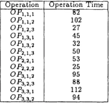
Table 1: J o b Requirements of Target System T h e operation time of each operation of jobs are shown in Table 2. In the table, OPj,;,k means t h a t it is an operation i of job j performed on machine
k.
Note that operation time includes tool set-up time of machine. Operation Time
B
z
102 2 7 45 32 50 5 3 25 95 88 112 94Table 2: Operation Time of Jobs.
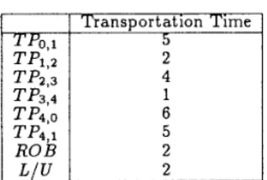
And, Table 3 gives the time of AGV’s transport& tion time between each pair of workstations or stops, e.g., T P ; , j means the transportation time from ma- chine Mi to machine
itl,.
Notice t h a t MO repre- sents the load/unload station. It also gives the load- ing/unloading time of stations, AS/RS, and AGV’s. And robot transfer time of the milling machine and lathe is also given. T h e symbolsL/U
and ROB are used t o represent the loading/unloading operation and robot transportation, respectively.T h e initial situation of the system is that all the machines, robot, AGV’s are all ready and available to
Transportation Time
5
2 4 Lot Sizes J o b 1I
J o b 2I
J o b 3 1 1 1 1 1Table 3: Transportation Time of Material Handling Systems
Total Completion Time 370
use. All the buffers, common or local, are also free. One AGV stays a t Loading/Unloading station, stop 0, and another one stays a t output port of AS/RS, stop 4.
In the heuristic search algorithm, the performance criteria we take is the total completion time, i.e. the makespan. This example is solved using the following heuristic function [5] :
h(n) = -w
*
d e p ( n )where 20 is a weighting factor and d e p ( n ) is set to be
the total number of accomplished operations for all jobs at node n. And the limited-expansion A algorith- m is used t o solve t h e job-shop scheduling problem.
Several different job sizes of this example are tested and the results
,
makespan only, are shown in Table 4. Note t h a t , the capacity of O P E N is limited to 16 and the weighting factor of heuristic function h ( n ) is set t o 3 in our limited-expansion A algorithm.2 2 ‘ 2 536
1403
Table 4: Scheduling Results (cost only).
5
Conclusions
In this paper, we use two basic sub-models to con- struct the complete Petri-net model of a n
FMS.
One is Transportation Model and the other is Process-Flow Model. T h e objective of Transportation Model is t o model the behavior of AGV traveling from the stop at which it currently stays t o its destination stop, which must also ensure t h a t collisions are avoided. And, the Process-Flow Model is used to model the behavior of the part routing and resource assignment.In order to obtain a n optimal schedule and to avoid the NP-complete computing complexity, we use a sub-optimal algorithm, limited-expansion A algo- rithm, based on the A* heuristic search algorithm.
This method not only can give solutions close t o the optimal or a near-optimal one, but also can easily be implemented on computers, since the memory require- ment is bounded and adjustable. For large volumes of parts, we propose a n adaptive scheduling method to be combined with the limited-expansion A search al- gorithm t o solve the scheduling problem.
References
[l] D. G. Catherine etc., “A Survey of Flexible Man- ufacturing Systemy,” Journal of Manufacturing System, Vol. 1, No. 1, pp. 1-16, 1982.
[2] Frederick A. Rodammer, K . Preston White, “A Recent Survey of Production Scheduling,” IEEE Transactions on Systems, Man, and Cybernetics, Vol. 18, No. 6, NOV/DEC 1988.
[3] Philippe Solot, “A Concept for Planning and Scheduling in An FMS,” European Journal of Op- erational Research, 1990, Vol. 45, pp. 85-95. [4] Simon France, Sequencing and Scheduling: A n
Introduction to the Mathematics o f the job-shop, New York:Wiley, 1982.
[5] D. Y. Lee, F. DiCesare, “FMS Scheduling Us- ing Petri Nets And Heuristic Search,” Proceed- ings of the 1992 IEEE International Confrerence on Robotics and Automation, Nice, France, pp. [6] Chin-Jung Tailand Li-Chen Fu, ”A Simula- tion Modeling for a Flexible Manufacturing System with Multiple Task-Flows and Trans- portation Control Using Modular Petri-Net Ap- proach”, Proc. 9th International Conference on CAD/CAM
,
Robotics & Factories of the Future, August, 1993.[7] N . J . Nilsson, Problem-Solving Methods i n Artifi- cial Intelligence, McGraw-Hill, New York, 1971. 1057- 1062.
stop0 stop4 stop3
+ - n
4 I 1 Machine Center U+
U stop1 stop2--m
Figure 1: Transportation System Layout of the