Nonlinear control of induction motor with unknown rotor resistance and load adaptation

Proceedings of the American Control Conference Arlington, VA June 25-27, 2001

Nonlinear Control of Induction Motor with Unknown Rotor Resistance

and Load Adaptation

Hou-Ban Lee', and Li-Chen

Fu'.'

1.

Department

of

Electrical Engineering

2.

Department of Computer Science and Information Engineering

,

National Taiwan University, Taipei, Taiwan, R.O.C.

E-mail

:

[email protected]

Abstract: On the basis of a dynamic model obtained under a special nonlinear coordinate transform on a d- q-axis model (w.r.t. the stationary reference flame) of an induction motor, a nonlinear adaptive controller for speed tracking control with unknown load torque is proposed in this paper. The controller is made to work under the condition that all the parameters except the rotor resistance of the induction motor are known a priori. The underlying control theories include the indirect vector control and the maximal power transfer of the motor. To be rigorous, the proposed control scheme is with a proof derived from Lyapunov stability theory. The simulation results are also given to show the effectiveness of the presented control scheme.

1. Introduction

The development of induction motor control can be generally categorized into two kinds. One is the improvement of power devices in both power electronics and microelectronics. The other is the development of various control schemes for both machines and drives.

The field oriented control (FOC) methodology is a popular control scheme of induction motor to achieve the high performance operation [l]

-

[3]. Field oriented control tries to deal with the induction motor as a DC motor to facilitate subsequent design of the high-performance control. After decoupling the nonlinear dynamical equations via the abc-to-dq coordinate transformation, the resulting controller structure can be much more simplified. Therefore, there are various kinds of control scheme developed to achieve the control objects based on FOC. The difficulty of the direct FOC is to detect the infonhation of rotor flux, since it costs a lot to measure the rotor flux extemally and usually the induction motors are without any built-in rotor flux sensors. Therefore, the control schemes based on indirect FOC are much more popular in applications. On the other hand, the issue of power efficiency of induction motor is well concerned nowadays [4]. Along this streamline of research, some results with focus especially on the power transfer to the rotor part have been presented earlier by the authors [SI [6].

In general applications, indirect vector control of induction motor is widely applied, where the rotor flux is estimated rather than being measured. This

requires a priori knowledge of the machine parameters, which makes the indirect vector control scheme machine dependent. Given the fact that parameters may change significantly with temperature and there are some states, which are not easily acquired, design of observer becomes crucially important to success of the control [7] [8]. Recently, the sensorless field oriented control scheme gradually appears as a popular control method for induction motors [9]-[ll]. Some of them even take the rotor resistance adaptation into the control scheme [9] [lo], but the complicated structures of the observers (or estimators) are often difficult to analyze and design. Taking the output (speed) feedback seemingly is another effective alternative dealing with the problem with unknown resistance [ 1 I]. On the other hand, the load torque structure is also a very important knowledge for controller design to achieve high performance control.

Given the above observation, we propose a speed tracking control scheme based on the indirect FOC with the property of maximal power transfer to the rotor. And, the proposed control scheme also handles the problems with both the unknown rotor resistance and torque adaptation. The rotor flux tracking is not considered here. The parameters of the induction motor except its rotor resistance are known as mentioned previously. For rigorousness, the developed control scheme is thoroughly analyzed via Lyapunov theory, and the asymptotic convergence property is soundly proved. The simulation results are given to validate the performances.

2. Maximal Power Transfer of Induction Motor

(A) Dynamical Model of Induction Motor

As has been'well known, the dynamical model of an induction motor can be simplified by a d-q-axis coordinate transformation from the original three phase representational frame to some rotational reference frame. But to make implementation feasible, the stationary-reference frame is more popularly used [12]. Thus, here we adopt the following group of (d-q- axis) coordinate-transformed dynamical equations of an induction motor

iqs = - adq,

-

PP@r/z,, -k cvqs i, = - a+,, i ppw,;l,, -k i c V,

where the states and the parameters are defined as shown in the nomenclature.

(B) Maximum Power Transfer

of

Induction Motor In order to develop the maximal power transfer of the induction motor, there is an assumption assumed as shown below:

(A.l) The induction motor is assumed without saturation, hysteresis, eddy currents, and spatial flux harmonics.

Theorem 1. (Maximal Power Transfer)

Under the assumption (A.I), ifthe input voltages in d- qfi-ame of the voltage-fed induction motor are defined as

. e

Then. thepower transferred to the rotor of induction

(V: + V i ) = (V / c ) * at any time. (see Ref. [ 5 ] , [ 6 ] ) motor is maximal subject to the constrain - - . .

Of course, V does not have to be a constant. Instead, it offers one D.O.F. (Degree of fieedom) control to the system, but normally it will converge to a constant (in regulation problem) or is related to the desired output (in tracking problem) when the system approaches to the steady state.

3.

Controller Design

For general mechanical systems, the load torque is

a function of the rotor speed q as:

= J L ~ + s ~ c + ) b 0 + b q +b2sgn(ur)c$

=JLca+L(4).

This assumption is more realistic

than

a constant load torque. For example, it can be shown that bearings and many othy viscous forces (including those encountered by cuttiug tools) vary linearly with speed, while large-scale fluid systems such as pumps and fans have loads that typically vary with the square of

the speed. In

this

paper, the mechanical load is assumed unknown, the sign function sgn() then can be neglected. Therefore, the mechanical load in the form aforementioned can be rearranged as TL =

OW:

with the

unknown

constant parameters

@=[J,

bo

4

41,

and known function vector

w,=

w sgn(w,) 0; sgn(w,)w;

.

The joint inertia J = J,

+

JL is therefore also unknown, and the damping coefficient can be assumed as apart of bl

.

In order to design the controller easily, we first introduce a reasonable assumption as shown below:

(A.2) x2 = A:r +Ajr > 0, then further simplify the dynamics shown in (1) by introducing a nonlinear state transformation given as Ref. [ 5 ] . Under the transformation, the dynamical equations shown in (1) can then be transformed to the following dynamic model:

[‘

1

XI = - 2a,x,

+

2a,x3

+

-

2ku, V

&

x2 = -2a,x2 +2a3x,

x3 = a3xl

+

a2x2 -(a,

+

a 4 ) x 3

+

px,x, i 4 =

-

pxsx3

-

(a,

+

a4)x4

+

&V

J x s = a+, - f L ( X s ) , (4)

where the parameters a,,a,,a,,a,,a, are defined in the nomenclature and the load structure- f L ( x s ) is well defined in the previous section. Note that the inertia of load is now coupled with the inertia of motof Since design of controller based on a particular system structure often involves complicated algorithms which may likely lead to

hi&

implementation cost, this fact thus motivates the need of designing a controller that can be applicable to a

vast class of system structure.

Lemma 1. Ifthe state variable xs =or, its derivative x5, and the stator current

Z,

are bounded, then states x i , i = 1,..,5, of system (4) are all bounded. Proof:

from system (4) as

First, we rearrange the dynamic equation of x2

x2 = -2a4x2

+

2a3(iqsAqr

+

ik&) I -a,x,

+

L;a,I:

,

where the positive pqameters a,,

a ,

are defined in the nomenclature and I,” = 1iS

+

I:

.

Thus x2 = A: =

Air

+ A i

is-boimded provided

Z,

is bounded.

And,

from system (4), if x, and its derivative are bounded, then x, is bounded immediately. As a consequence, all the states x,, x2 and x, , which are composed of bounded signals I, and

il,,

are

In the following theorem, we relax the knowledge therefore concluded being bounded. QED.

L, A

V=-

of both the load torque and rotor resistance.

Theorem 2. Consider an induction motor whose then it will lead to the result that dynamics are governed by system (4) with unknown

load torque and rotor resistance under the = -Pie:

-

P 2 4 . Hence,

r‘,

< 0 with PI P2 > 0 . assumptions (A.l) and (A.2). Given a twice- Thus, we conclude all the error signals

h

Ve and, in differentiable smooth desired speed PUJeCtOty #d particular, x5 and X4d are bounded, in turn

with and i j d are all bounded then the implies that x , and 2, (from system (3)) are following control input can achieve the control _bounded.

_id

_{is bounded since}

_B~

_{is bounded.}

objective 0,

+ad

(i.e. x, =or will follow CO,

By Lemma 2, we thus conclude all the intemal signals are kept bounded. With

Cii,

being bounded as the a.ymptotical&) with the control input

requirement, x4bd is hence bounded. Therefore, all the composed states of V are independent of K Then

all the boundedness of the composed states of V will -Ae4l be kept with a sufficiently large

llql.

Obviously, the

[(a, +a4)x4 +px& +x,d+-Rd x4 -use5 -pze4I 9

&

D

, lf; =

c,

and

I/

=A-

Y

95 J W C J W C

1 L, A

V=---[(a,

A

+a44)x4 +P?& + X 4 d + - R d x4

D L A

, where Rd = R , - R, ,

xdd = -(bo+ bl x,

+

bz x:

+

J CUd- p,e,) with 1 A A A A.

a5

. A

2 2 = -e,x:,

j

=-e, W d , R d = - L e 4 x 4 , while all

D the internal signals are kept bounded Proof:

In order to show the boundedness of all the parameter estimators and the tracking errors

e,, e,

, we choose a Lyapunov function as shown below:

1

2

=-[J4

+e:

+it

+ p

+6:

+?

+(&-&)’I,

where Rd =R,-R,. Whose time derivative is obtained

as

follow:

Y e =e,a,x4 -e,( bo +b,x, +b&) --Ji?gm+ed(x4-x4d)

.

. .

.

.

A - A - A - A A

+ i o

bo

+

bi b,

+

bz b2 + J J

+

R d ( R d - R,) .

If we design the parameter adaptive laws as

bo = -e5, b, = -e5x,, b2 =-e,.:, J =-e, W d ,

i d = - L e 4 x 4 along with the proper design of x4a

as x , ~ = -(bo+bl x, +bz x:

+

J w d - p , e , ) , then the

time derivative of the Lyapunov function V, becomes

V , =-p,e: +e4[-(a, +a,)x4

-px,x,

A A A A

D

A .

1 * A

a,

Ed

=

id

-

Rd

.

Now, design the actual input

bounds of x, and xs are only independent on the initial conditions involved in J f e , rather

than

on J f

particularly. From the power formula, ,dr and 1 9 s

should be in the order of if gets large. To continue the proof, we first assume that V is unbounded, ids and i,, are then bounded, which together with earlier boundedness thus implies boundedness of all signals x,, i = 1 ,.., 5. On the other hand, if V is boundedness then, since

P,

=a, x., x, = 3

YZ,,

I , is bounded, and the rest of proof will then follow the previous. Now we can show that e5 is bounded since i, and ~d are bounded,

which implies the convergence of e, due to

Barbalat’s Lemma. Certainly, the tracking objective (speed tracking) is achieved with e, +O as t

+

CC

(concluded from Barbalat’s Lemma). Therefore, the control scheme

with

the properly designed input I f will drive the output w, to the desired ad

asymptotically. QED.

4.

Simulation Results

Iv

I

In this section, the performance of the developed controller, as it is applied to an induction motor, will be demonstrated by a number of simulation examples. The characteristics of the motor are listed as below: R, = 0.83!2, R, = 0.53!2, L, = O.O8601(H),’ L, = O.O8601(H), L, = 0.08259(H), J, = 0.033 (Kg-m’),Q poles, mted current 8.6

A,

220 V, 60

Hz,

AC.

The mechanical load torque is chosen to be T, = JLkr

+

b,

+

b m ,

+

b m ; , whose parameters are assumed as follows: JL = 0.01, bo = 1.0, b, = 0.1, b2 =

0.001. For practical implementation, the amplitude of the input voltage is limited and the upper bound of the input voltage is 300

V.

The desired speed commands

ad

are described in the following cases and the control gains are p, = 1000, and p, = 500.

( I ) =30(1-exp(-lOt)) (radsec)

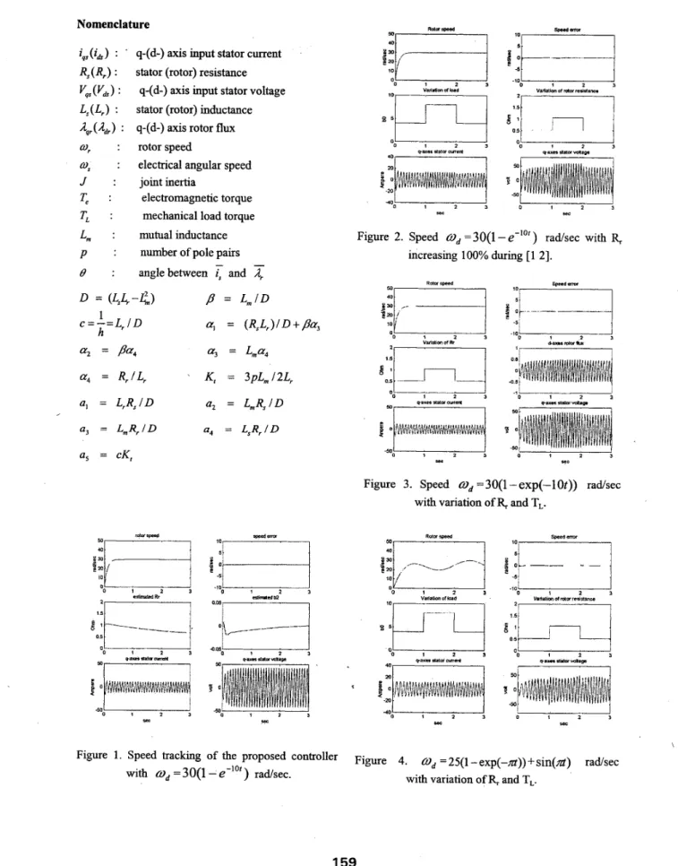
Figure 1 shows the speed tracking with unknown rotor resistance and load torque parameters. The estimated Rr and b, are shown bounded. In order to show the robustness of the controller with respect to variation of rotor resistance and load structure, we then have the simulation cases as follows:

(2) Variation of

R,

The speed command is designed as in case (l), but the rotor resistance is increasing 100% during the time interval [I 21. Figure 2 shows the effects of the proposed control scheme. Obviously, the input stator voltage is increased to suppress the variation of the rotor resistance.

(3) Variations of both rotor resistance and load torque The speed command is designed as in case (l), but both

R,

and T,, are changed. The parameters of load torque are assumed unchanged except bo. Both

R,

and bo are increasing 100% during the time interval [l 21. As shown in Fig. 3, Both the stator voltage and current have been varied to overcome the variations. The speed tracking is still well achieved.

(4) @, =25(1-exp(-nt))+sin(nt), with variations of both

R, and TL

As the speed command w, being a composed time varying function, the control objective is also satisfied. Fig. 4 shows the performance of the controller with the same variations of both R, and TL as in case (3).

and a set of nonlinear transfoxmation.

Reference

5. Conclusion

In

this

paper, we first develop a special nonlinear coordinate transform which makes the rotor flux norm, the electric torque and the rotor speed as individual variables x,, x., and x , , respectively. Then, we propose a field-oriented Lyapunov-based controller for an induction motor with the property of maximal power transfer. And, it can also deal with both the

unknown rotor resistance and the unknown load torque. Numerical simulations and experimental results validate the performances mentioned above. There are some concluding remarks should be s-ed

as

below:

1. The proposed control scheme of induction motor, which copes with unknown rotor resistance and

unknown load torque, is a Lyapunov-based design. 2. The load torque structure is assumed as

TL

=

JL

wr+ bo

+

blw,

+

bm; with the unknown constant parameters 0 =

[

.IL

bo bl b2]

.

3. The proposed control scheme is developed based

on the maximal power transfer of induction motor

15

[l] R. Marino, S. Peresada, and P. Tomei, ”Global Adaptive Output Feedback Control of Induction Motors with Uncertain Rotor Resistance,” ZEEE Trans. Automat. Con&, Vol. 44, No. 5, pp. 968- 983,1999.

[2] H. Tajima, and

Y.

Hori, “Speed Sensorless Field- Orientation Control of Induction Machme,” IEEE Trans. Zndust. Appl., Vol. 29, No. 1, pp. 185-180, 1993.

[3] G. Espinosa, R. Ortega, and P. J. Nicklasson, “Torque and Flux Tracking of Induction Motors,” Znt. J. Robust & Nonlinear Conk, Vol. 8, pp. 1-9,

1998.

[4] G. S . Kim, I. J. Ha, and M. S.

KO,

“Control of Induction Motors for Both High Dynamic Performance and High Power Effiency,” ZEEE Trans. Zndust. electron., Vol. 39, No.4, pp. 323- 333,1992.

[5] H. T. Lee, L. C. Fu, and H. S. Huang, “Speed Tracking Control with M a x k l Power Transfer of Induction Motor,” Pmc. 3Yh ZEEE Con$

On

Decision and Control, pp.925-930, 2000. [6] H. T. Lee, J. S Chang, and L. C. Fu, “Exponential

Stable Nonlinear Control for Speed Regulation of Induction Motor

with

Field Oriented PI- Controller,” Int.

J.

Adap. Conk & Sign. Proc., [7] R. Krishnan, and A.

S.

Bharadwaj, “A Review of Parameter Sensitivity and Adaptation in Indirect Vector Controlled Induction Motor Drive Systems,” IEEE Trans. Power Electron., Vol. 6,

[8] M. H.

Shin,

and etc., “An Improved Stator Flux Estimation for Speed Sensorless Stator Flux Orientation Control of Induction Motors,” ZEEE Trans. Power Electron., Vol. 22, No.2, pp. 321- 318,2200.

[9] H. Kubota, and K. Matsuse, “Speed Sensorless Field-Oriented Control of Induction Motor with Rotor Resistance Adaptation,” IEEE Trans. Zndust. Appl.. Vol. 30, No. 5, pp. 1239-1244, 1994.

[lo] R. M. Marino,

S.

Peresada, and P. Tomei, “Adaptive Observer-Based Control of Induction Motor with Unknown Rotor Resistance,” Znt. J. Adapt. Conk & Signal Proc., Vol. 10, pp. 345- 363,1996.

[11] R. M. Mario, S. Peresada, and P. Valigi, ‘‘Output Feedback Control of Current-Fed Induction Motors with Unknown Rotor Resistance,” IEEE Trans. Con& Syst. Tech., Vol. 4, No. 4, pp. 336- 347,1996.

[12] P. C. Krause, Analysis of Electric Machinely, McGraw-Hill, 1986.

Vol. 21, NO.213, pp. 297-321, 2200.

-

No.4, pp. 434440, 1990.

-Nomenclature

q-(d-) axis input stator current stator (rotor) resistance

q-(d-) axis input stator voltage stator (rotor) inductance q-(d-) axis rotor

flux

rotor speed

electrical angular speed joint inertia

electromagnetic torque mechanical load torque mutual inductance number of pole pairs anglebetween

<

and

7

D =

(4443

c = -= L, I D

a,

= (RsLr)/D+,Ba3 a 2 =

Pa,

a, = Lma4

a4

= R,/L, ' K , = 3pLm /2Lr a, = L,R,/D a, = L m R s / D ,B = L m / D 1 h a3 = L,,,R,/D a4 = LsRr I D a5 =

cK,

:k---i

I I 0 I 2 3 M

Figure 2. Speed W,

=30(1-e-'")

radsec with R, increasing 100% during [l 21.

Figure 3. Speed W,

=30(1-exp(-lOt))

radsec with variation of

R,

and TL.