多媒體內容傳遞網路前瞻技術之研究-子計畫二： 對等式內容網路之搜尋與傳遞演算法及安全議題研究(2/2)

行政院國家科學委員會專題研究計畫 成果報告

子計畫二：對等式內容網路之搜尋與傳遞演算法及安全議題

研究(2/2)

計畫類別： 整合型計畫

計畫編號： NSC93-2213-E-002-057-

執行期間： 93 年 08 月 01 日至 94 年 07 月 31 日

執行單位： 國立臺灣大學電信工程學研究所

計畫主持人： 林宗男

報告類型： 完整報告

報告附件： 出席國際會議研究心得報告及發表論文

處理方式： 本計畫可公開查詢

中 華 民 國 94 年 9 月 28 日

行政院國家科學委員會補助專題研究計畫

■ 成 果 報 告

□期中進度報告

多媒體內容傳遞網路前瞻技術之研究-子計畫二：

對等式內容網路之搜尋與傳遞演算法及安全議題研究(2/2)

計畫類別：□ 個別型計畫 ■ 整合型計畫

計畫編號：NSC93－2213－E－002－057

執行期間：93 年 8 月 1 日至 94 年 7 月 31 日

計畫主持人：林宗男教授

共同主持人：

計畫參與人員：

成果報告類型(依經費核定清單規定繳交)：□精簡報告 ■完整報告

本成果報告包括以下應繳交之附件：

□赴國外出差或研習心得報告一份

□赴大陸地區出差或研習心得報告一份

□出席國際學術會議心得報告及發表之論文各一份

□國際合作研究計畫國外研究報告書一份

處理方式：除產學合作研究計畫、提升產業技術及人才培育研究計畫、

列管計畫及下列情形者外，得立即公開查詢

□涉及專利或其他智慧財產權，□一年□二年後可公開查詢

執行單位：國立台灣大學電信工程學研究所

中

華

民

國

九

十

四

年

九

月

二

十

七

日

中文摘要

本研究計畫對於如何衡量搜尋網路效能的諸多重要議題做深入思考。現有的評量

標準可能會對於搜尋的效能做出偏頗的結論，或是對於演算法的設計提供錯誤的方

向。因此，我們定義一個統一的準則，稱之為「搜尋效能」(Search Efficiency, SE)，

以綜合廣泛的方式來處理搜尋效能的問題。SE 的目標在於更充分的描述搜尋網路效能

的特性，並對未來的設計提供方向。我們首先在一個理想的網路拓墣，strictly binary

tree，藉由分析 SE 在兩種典型的搜尋方法，包括 breadth first search 以及 random

walk，來驗證 SE 的正確性。另外，基於各種不同的網路狀況，我們進一步展現 SE 在

真實世界網路拓墣，power-law random graph，描述效能特性的能力。最後，基於 SE

的分析，我們設計一個演算法，dynamic search。Dynamic search 展現出的優異性能，

對於 SE 提供未來搜尋網路設計方向的能力做出絕佳示範。

關鍵詞

英文摘要

This project deliberates on various critical aspects in evaluating

searching networks. Existing metrics either draw biased conclusions regarding

search performance or provide wrong guidelines for algorithm design. We,

therefore, define a unified criterion, Search Efficiency (SE), to objectively

address search performance in a comprehensive manner. The goal of SE is to

better characterize performance of searching networks than existing metrics

do as well as to guide the design of future ones. We first validate the

correctness of SE in performance evaluation in an ideal graph, strictly binary

tree, by analyzing SE for two typical search methods, breadth first search and

random walk. We further show its strength in performance characterization in

the real-world topology, power-law random graph, under various network

conditions. We finally design an algorithm, dynamic search, based on SE

analysis. Its proved outstanding performance demonstrates the strength of SE

to provide guidance for the future design of searching networks.

Keywords

目錄

中文摘要... II

英文摘要... III

目錄...IV

前言... 1

研究目的... 2

文獻探討... 3

研究方法... 4

結果與討論... 12

結論與建議... 16

參考文獻... 17

附錄... 18

前言

Searching networks, including social networks and computer networks, play

an increasingly important role in human activity. A significant example is the

recently popular peer-to-peer (P2P) file-sharing systems, e.g. Gnutella and

KaZaA, where every peer collaboratively forms a searching network to locate

desired files by a real-time search. In the social context of searching networks,

people search their acquaintances for a particular item or expertise in a

specific domain. Their acquaintances in turn report whether they have the

desired item (expertise) or subsequently deliver this query to their next-step

acquaintances. In this fashion, a social searching network or so called human

acquaintanceship graph [8] is formed. Thus, a searching network is a system

where each participant contributes to the network and collaborates to help

others search targeted resources.

In a searching network, one of the critical issues is to maximize search

performance by choosing or designing algorithms used to perform the search

process. Novel algorithms [5, 6, 7] have been proposed to address different

search aspects, such as success rate, search cost, coverage, or number of hits,

but an objective and comprehensive evaluation metric is missing. As a result,

these algorithms tend to be designed with biased considerations and evaluated

in limited dimensions.

研究目的

In summary, our objectives are stated as follows:

n

We propose a unified and objective metric, Search Efficiency, for

evaluating searching networks and characterizing search algorithms.

n

We mathematically analyze critical performance metrics—search

coverage, cost, success rate, number of hits, and SE—in searching

networks.

n

We analytically evaluate various algorithms, including BFS, M-BFS, RW,

and a novel search, in SBT and PLRG, under uniform and non-uniform

object distributions.

n

We devise a new search algorithm, dynamic search, based on the

knowledge from temporal SE analysis. It is shown to outperform other

existing ones, thus SE proved to provide solid guidance for algorithm

design.

文獻探討

Breadth-first search (BFS) and random walk (RW) [5] are two basic and

typical search methods in searching networks. BFS inherently maximizes the

search speed and coverage but risks generating search queries in an

uncontrolled (exponential) manner. RW, on the other hand, minimizes search cost

but generates limited search coverage and results. As a result, one might draw

distinct conclusions about algorithm performance, if different metrics are

concerned. For example, Gkantsidis et al. [12] claimed RW performs better than

BFS in terms of number of hits and failure probability give the same search

cost for BFS and RW, but implicitly assumed an infinite search time for RW,

which is clearly unfair. Jiang et al. [9] evaluated their proposed search scheme

only by search coverage and message cost, leaving search speed and success rate

unchecked. Lv et al. [5] provided a spectrum of aspects on evaluation, but

analyzed them individually and still lacked an overall consideration.

Our work, therefore, deals with these one-sided perspectives and

synthesizes a unified search criterion, Search Efficiency (Section II), which

is critical particularly in P2P endeavors, to objectively evaluate search

algorithms and provide overall guidance for the design of searching networks.

With the unified metric SE, we first validate its correctness by deriving

its mathematic formulas for BFS and RW in a simple topology, strictly binary

tree (SBT), and analyzing whether the performance indicated by SE is reasonable.

Furthermore, we extend the results of Newman [1] and Adamic [2] and further

consider “redundancy” to analytically approximate SE for BFS, M-BFS [14],

and RW in a power-law random graph (PLRG), which is shown to be the real topology

of current searching networks. We thus validate SE in comparison with previous

simulation works [5, 9, 11], deliver the unique performance characterization

of SE, and provide in-depth analysis.

Throughout the analysis in this project, we compare various existing

metrics with SE to address their limitation and strength. We show that no matter

in SBT or PLRG, existing metrics draw biased conclusions regarding search

performance; they either provide one-sided considerations or deliver wrong

guidelines for algorithm design. Moreover, they fail to characterize

performance variance under distinct network conditions, such as object

replication ratios (Section III) and object distributions (Section VI).

In the final analysis, we propose a new algorithm, dynamic search, based

on the results of SE analysis. We prove this algorithm outperforms existing

ones and SE effectively provides guidance for algorithm design.

研究方法

SEARCH EFFICIENCY

We argue that to best characterize the efficiency of any system is to measure its ability to transfer its input to generate meaningful output, which is applicable in the evaluation of search methods performed in any network. In a social network, the input of a search largely involves the cost required for querying process including costs of phone calls, transportation, and even consulting. As for output, it should be measured by searchers’ satisfaction in terms of the chance of success, the response speed, and quality of responsive results. To clarify the definitions of and relations between these inputs and outputs in the context of searching networks, we start a series of discussions about Search Efficiency with Query

Efficiency (QE).

A. Query Efficiency

In general, the most critical aspects of search performance involve the extent of search coverage (output) [2] and the cost required to cover the network (input) [5]. By search coverage, denoted as Coverage or C, we mean the number of distinct or effective peers visited by search queries, i.e. we do not count the repeatedly visited ones. In addition, by cost, denoted by QueryMsg, we mean the number of queries incurred, for it is a representative factor to which other cost factors (e.g. computer processing power or costs for phone calls and transportation) tend to be proportional. Thus it is trivial to say a search which uses S query messages to traverse distinct S nodes is perfectly or 100% efficient in terms of query generation. Additionally, we can define a sort of efficiency as Coverage / QueryMsg. However, the end goal of searching is not to cover as many nodes in the network as possible. Rather, its ultimate goal is to search out the desired targets or objects, in which covering is only one of the adequate conditions (e.g. cache or previous experience) for that end. This is true when the searching network is well-designed, e.g. Chord [13], such that large search coverage is not necessary, or when object distribution is not uniform in which directed search is preferred. We will show performance difference between Coverage and

QueryHits under non-uniform object distribution in Section VI.

Thus, we define QueryHits(t) as the number of desired objects found “at” search time t, which is measured by the number of hops or depths, to quantify the yields of a search. We introduce the factor search time t for the purpose of future discussion. Again, we might define the efficiency of queries as ?tQueryHits(t)/QueryMsg. However, this definition is sensitive to the population of desired objects, which

is irrelevant to the performance of search algorithms themselves and should be factored out. For this purpose, we introduce the notion of object replication ratio R defined as the ratio of the number of targeted objects to the network size (N). To cancel the population factor out, we normalize it with respect to R and thus formulate Query Efficiency (QE) as

1 ( ) 100% (%) , TTL t QueryHits t Query Efficiency QueryMsg R = = ∑ ×

(1)

where TTL refers to the termination condition of searches, measured in hops. To exemplify, we suppose a search consuming 100 messages to find 1 targeted object in a network with R of 1%, which reveals that

1% of nodes have the desired object. By

(1)

, QE = 100% and we thus call it a perfectly query-efficient

the search effectively covers 100 nodes (from 1/1% = 100) and this provides a clear view of the perfect efficiency.

B. Responsiveness

One of the goals of searching, as addressed previously, is to find out possible objects while the other is to find them as soon as possible. We define search response time, denoted by t, measured by discrete numbers of hops, to evaluate the speed of searching objects, or responsiveness of a search. If a search finds Q desired objects in its hth step or in its hth-nearest acquaintances, we denote it as QueryHits(t=h)=Q.

We argue that a search getting hits in a faster fashion delivers better users’ experience and should be gauged as higher reputation. More specifically, responsiveness of a search should be inversely proportional to the response time t. To consider this factor for SE, we may simply divide QE by the

weighted response time, which is computed by ?t[t·QueryHits(t)] / ?tQueryHits(t). However, this method

would generate unjust results. For example, we assume a search that uses 1000 messages to get 99 hits at t = 1 and 1 hit at t = 100 with R = 10%, resulting in a weighted response time of (1·99+100·1)/100 or 1.99. According to QE in (1), if we don’t count the hit at t = 100, the search is 99% query efficient, but it dramatically reduces to 50.25% efficiency due to dividing by response time 1.99 when that hit is calculated. This method unreasonably emphasizes the slow search hit. We argue that any query hits contribute positively to the search itself despite long response time. We thus aggregate these responsive hits rather than divide by the averaged response time to give efficiency as

1 ( ) / 100% TTL t QueryHits t t QueryMsg R = _× ∑ _.

The efficiency of this example becomes 99.01% rather than 50.25%, where the last found hit contributes 0.01% to efficiency, rather than severely reducing it.

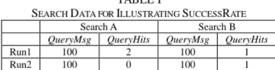
C. Reliability

The last concern is reliability, which is measured by SuccessRate in our design of SE. We introduce it so as to further consider the satisfaction of user experience. Consider two searches (A and B), each performing two runs, as shown in Table I. We assume all objects are found at the same response time. The success rate of Search A is 50% while B is 100%.

TABLE I

SEARCH DATA FOR ILLUSTRATING SUCCESSRATE

Search A Search B

QueryMsg QueryHits QueryMsg QueryHits

Run1 100 2 100 1

Run2 100 0 100 1

Note that if we compute efficiency without SuccessRate, we will gain the same result for Search A and B. However, one of the runs in Search A (Run 2) fails and thereby we neglect to measure the penalty of user experience in Run 2. By introducing the term SuccessRate, SE of Search B remains the same, but SE of A is halved. In this manner, it successfully addresses the user satisfaction level while the two searches get the same number of hits at the same message costs. In sum, the term SuccessRate is aimed to successfully measure the satisfaction level from users’ perspective. Finally, we define the overall criterion

for evaluating searching by 1 ( ) TTL t QueryHits t t SuccessRate Search Efficiency QueryMsg R = = ∑ × ,(2)

where TTL stands for the limit of search covering.

D. Limitations of Search Efficiency

The design goal of SE is to capture a simple but representative view of search performance. As a result, it is possible to consider more complex considerations for search evaluation. We list three possible aspects that are not covered by SE:

1) In the context of computer searching networks, the implementation of caches or DHT would significantly improve the search performance, which SE could reflect. However, SE doesn’t consider the additional resources (processing power or memory) required by performance-boosted mechanisms, such as hash functions or caches, thus potentially overestimating the efficiency of algorithms adopting these additional mechanisms.

2) The costs of searching each computer or peer should not be equally weighted. Consulting an institution for recommendations is clearly more costly than asking a close friend, although we only assume they are equally costly.

3) We make a limited measure of responsiveness by the factor t. For instance, it would be more flexible using ta, a > 0, to adjust the extent to which search responsiveness is concerned.

By means of Search Efficiency, we can objectively evaluate performance of algorithms in searching networks. In the remaining of this report, therefore, we aim to characterize various existing search algorithms in terms of SE and demonstrate the biased view of existing search metrics compared with SE. In the following sections, we will mathematically derive the formulas for SE in the context of three basic search approaches, BFS, RW and M-BFS, the variation of BFS, in two representative topologies, the strictly binary tree (SBT) as well as the power-law random graph (PLRG), in order to demonstrate the strength of SE.

STRICTLY BINARY TREE

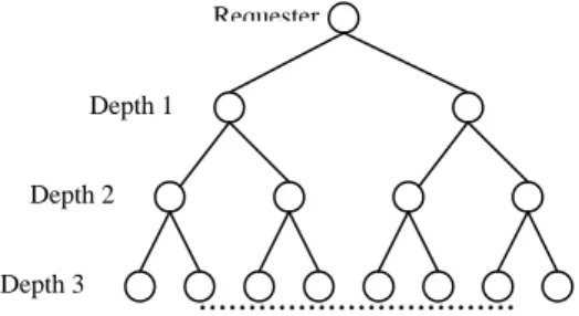
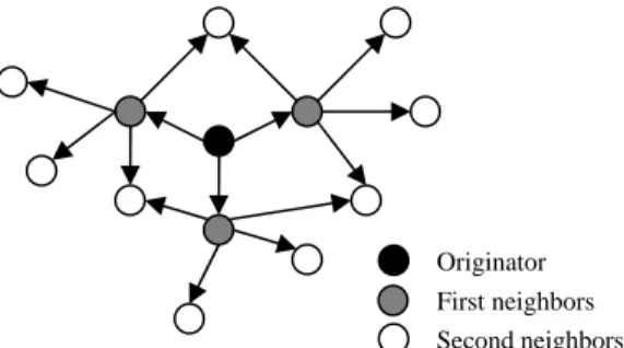
We assume an N-vertex strictly binary tree whose depth is about log2N and that the requester is at the

root such that the response time (t) of a query hit is the same as the depth (d) where the target object is located. This tree is shown in Fig. 1. Moreover, for simplicity of analysis, we assume objects are uniformly distributed in the tree or graph until Section VI.

Before analyzing specific algorithms, we first prepare two common factors for the derivation. Firstly,

the number of objects searched out (QueryHits) is proportional to the search coverage C. Thus, we have

QueryHits= ×R C. (3)

Secondly, the success rate of a search is also relevant to the search coverage. To begin with, we know that each node owns the target object with a probability of R; that is, each node lacks the object with a probability of 1- R. Suppose a search covers C vertices and thus the probability these C nodes share no

targeted object is (1- R)C. Inversely, the probability these C nodes share one or more objects, or

equivalently SuccessRate, is determined by

1 (1 )C SuccessRate= − −R . (4)

A. Breadth First Search in Strictly Binary Tree (SBT)

Analytic Derivation:

Breadth-first search (BFS) performs by broadcasting the received queries to all neighbors except where the received query came from. Therefore, by the regular structure of a strictly binary tree, the search coverage terminated at depth TTL is given by

1

( ) TTL_t 2t

Coverage C =∑₌ (5)

Furthermore, the number of messages required to traverse the tree is the same as the quantity of its

search coverage due to the very nature of BFS. Thus, QueryMsg = C = ?t 2

t . According to

(1)

,

(3)

, and

(5)

, we attain 1 1 2 100% 100% 2 t TTL t BFS TTL t t R QueryEfficieny R = = ⋅ = ∑ × = ∑ (6)

...

Fig. 1. A strictly binary tree with the requester at the root Depth 2

Depth 3 Depth 1

Requester

Search Efficiency for BFS

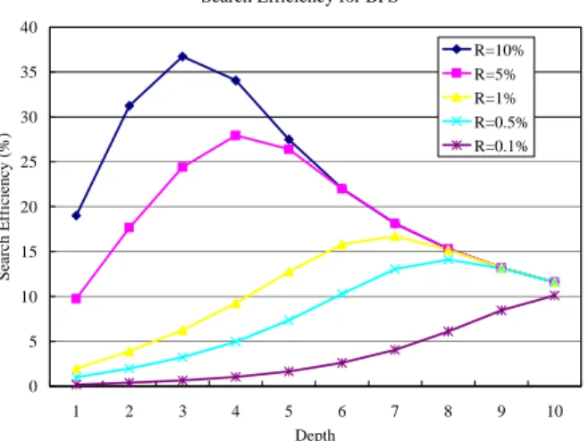
0 5 10 15 20 25 30 35 40 1 2 3 4 5 6 7 8 9 10 Depth Search Efficiency (%) R=10% R=5% R=1% R=0.5% R=0.1%

Fig. 2. Search Efficiency for BFS terminated by incremental TTLs (Depth)

in a strictly binary tree with various replication ratios R

Surprisingly, the formula of QEBFS yields a constant, 1 or 100%, regardless of the replication ratio R or

the termination depth TTL. By the definition of QE, this means that BFS is a perfectly query-efficient search in the context of a binary tree; that is, BFS generates no redundant messages while traversing a binary tree. The idea of redundancy will be further defined and discussed in the next section.

Finally, the general formula of SE defined in (2) for BFS in a binary tree is

(

)

12 1 1 2 1 1 . 2 t TTL t t TTL t BFS _{TTL t} t t SE = R ∑= =   = × − −_{ }   ∑ ∑ (7)

The derived SEBFS is complex for one to gain insight of its properties due to the running variable t and

various possible values of R. To deliver a clearer understanding, we assume the replication ratio R << 1,

which is true in real searching networks, and approximate

(7)

as

(

)

[

]

∑ ∑ ∑ = = = = _{× − − ⋅∑ = ⋅} ≅ TTL t t TTL t t TTL t t TTL t t BFS R R t t SE _{1 1} 1 1 _{1 1 2 2} 2 2 .

(8)

Search Efficiency Analysis:

To exemplify SEBFS, we set R = 0.1% (far less than 1) and obtain by

(8)

SETTL=1 = 0.2%, SETTL=2 = 0.4%, and SETTL=3 = 0.67%. Note SE is strictly increasing with respect to

TTL— SETTL=2 is exactly twice of SETTL=1 and SETTL=3 is more than three times of SETTL=1. The reasons are

two-fold. Firstly, as formula

(6)

shows, BFS in a binary tree is perfectly query-efficient, which means

every query positively contributes to its search coverage and in turn produces promising increase in SE. Secondly, the speed at which query hits are returned is faster than the decay factor of response time t.

Furthermore, formula

(8)

tells that the benefits from BFS are increasingly proportionally to 2t while the

factor t is used to compensate the demerit of long search time, where the factor 2t tends to dominate. Thus

we conclude every query or every additional covered depth makes a positive contribution to the overall performance despite the compensation of time, given that the replication ratio is much smaller than unity.

We present analytically-derived data of SEBFS, without approximation, by

(7)

with a spectrum of

parameters, Rs and TTLs, in Fig. 2. Firstly, we note that SEBFS for all Rs approaches some fixed level in the

long run. This fixed level, obtained by

(7)

for large t, is determined by the characteristic of the searched

topology— strictly binary tree— that is irrelevant to R. Second, the short-term increase of SE for high R (10% or 5%) results from the perfect query efficiency and popularly distributed objects, while the

long-term decrease is due to the compensator of response time t. If we use the notion ta suggested in

Section II.D, where a is 0 or small for some application scenarios and responsiveness is of little concern,

SE in

(7)

will increasingly grow to some fixed level. Third, as for low R (0.1% or 0.5%), the results in Fig. 2 are reflective of the discussions in the above paragraph— SE is consistently increasing.

Note that, however, if we take TTL as infinity in

(7)

, it gives zero seemingly contradicting our notion. In

reality, however, TTL cannot be infinity but is generally 7~10, in which SE still generates a fixed level of performance reflecting the characteristics of SBT.

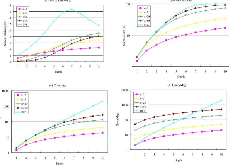
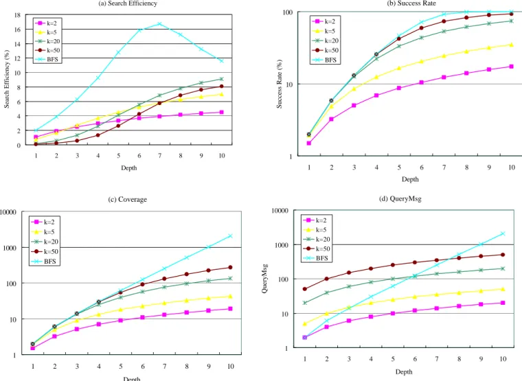
Fig. 3. Performance comparison by various metrics— (a) Search Efficiency, (b) SuccessRate, (c) Coverage, and (d) QueryMsg— for RW of various number of walkers k and for BFS in a strictly binary tree with R = 1%

Metrics Analysis:

We compare two metrics, SE and Coverage in this scenario. The results of

Coverage of BFS can be referred to in Fig. 3(c). If we take only Coverage (C) into consideration, it

produces the same performance in spite of different extents of object replication (different values of R)

since C by

(5)

is independent of R. Hence, Coverage fails to characterize the performance variance in

searching networks with different replication ratios. On top of this, if the design goal is to maximize C, then one may conclude that the choice of termination condition TTL is the larger the better— an impractical conclusion. On the other hand, if we only inspect QueryMsg, we will get entirely opposite conclusions. Therefore, Coverage and QueryMsg draw contradictory conclusions and fail to provide comprehensive guidance.

In fact, by the indication of SE in Fig. 2, TTL should be small when R is large in order to avoid unnecessary message propagation when R is large and to generate satisfactory results when R is small. In sum, SE better characterizes performance and provides a better guideline of TTL design than Coverage and QueryMsg.

B. Multiple Random Walks in Strictly Binary Tree

When it comes to RW search, we use multiple “walkers” to traverse the network and the number of walkers is denoted by k. Each walker independently searches the network and randomly chooses one of the next-hop neighbors to continue its journey to the limit of TTL hops.

(a) Search Efficiency

0 2 4 6 8 10 12 14 16 18 1 2 3 4 5 6 7 8 9 10 Depth Search Efficiency (%) k=2 k=5 k=20 k=50 BFS (b) Success Rate 1 10 100 1 2 3 4 5 6 7 8 9 10 Depth Success Rate (%) k=2 k=5 k=20 k=50 BFS (c) Coverage 1 10 100 1000 10000 1 2 3 4 5 6 7 8 9 10 Depth Coverage k=2 k=5 k=20 k=50 BFS (d) QueryMsg 1 10 100 1000 10000 1 2 3 4 5 6 7 8 9 10 Depth QueryMsg k=2 k=5 k=20 k=50 BFS

Analytic Derivation:

To begin with, we consider Coverage to derive SE. We know each vertex at

depth t is visited by a random walker with equal probability, 1/2t. Moreover, each random walker

independently makes its own decisions to traverse the topology. Thus, the probability that all k walkers

don’t visit a certain vertex is (1- 1/2t)k. As a result, at depth t, the average number of nodes visited

(Coverage per Depth) by k random walkers is given by the expectation

1 ( ) 2 1 (1 ) 2 t k t t E X = _ − − _  . (9)

By (3), QueryHits(t) = R·E(X)t. Moreover, the query messages of random walk are generated per hop for

each walker until terminated by the TTL limit, hence

QueryMsg = k·TTL. (10)

As a result, QE of k-random walk is

1 ( ) 1 ( ) TTL TTL t t t t RW k R E X E X QE k TTL R k TTL = = = ⋅ = = ⋅ ⋅ ⋅ ∑ ∑ _{. (11)}

Furthermore, from (4), we obtain

1 ( )

1 (1 )C 1 (1 ) TTLt E X t. SuccessRate= − −R = − −R ∑= (12) Therefore, Search Efficiency for k-random walks is

(

)

1 ( ) 1 ( ) / _{1 1} TTLt t _, TTL E X t t RW k E X t SE R k TTL = ∑ = = =

∑

_× × − −_ _ (13)

where E(X)t is determined by (9).

Search Efficiency Analysis:

Assuming R = 1%, we generate a series of performance results of SE in terms of various numbers of walkers k. We thus plot these results of SE (13), SuccessRate (12), Coverage (9), and QueryMsg (10) for RW and BFS in Fig. 3.

In Fig. 3(a), we observe that all SEs of RW consistently increase with respect to the depth or search time. Nevertheless, they all are smaller than that of BFS due to too many (redundant) query messages in the local search, and the slow covering and low SuccessRate in the long-term search. Therefore, they fail to utilize the regular structure of SBT. As for the number of walkers k, a too large (e.g. 50) or too small (e.g. 2) value of k gives degraded performance, thus resulting in strong sensitivity in the choice of k.

Metrics Analysis:

By merely inspecting Fig. 3(b) for SuccessRate or (c) for Coverage, one may jump to a conclusion that the number of walkers k is the larger the better. This aspect disregards the fact that larger k would generate larger search cost, shown in Fig. 3(d), and potentially redundant query messages. In fact, comparing RW of k = 50 and of k = 20, we find that their values of SuccessRate or Coverage during depth t = 1~4 are almost the same while the former generates 2.5 times more search cost— the latter search uses less search cost to produce similar search fruits. In consequence, in the short-term search, the latter one should be gauged as better search. Thus the conclusion larger k is better for RW would be fallacious. Therefore, we argue that neither SuccessRate nor Coverage is a good performance indicator.

Moreover, the long-term performance will inherent the short-term so that SE in Fig. 3(a) well characterizes the better performance for RW of k = 20. Besides, RW of k = 2 would be the best search in Fig. 3 if we try to minimize QueryMsg and scalability is the most concerned issue. Yet, this would be a specious conjecture since it entirely flies in the face of the final end of search— to find the results responsively.

C. Summary of Search Efficiency in SBT

By the discussion in this section, we validate SE by showing 1) the 100% QEBFS indicates that BFS

perfectly utilizes the regular structure of SBT and generates no redundant messages, 2) the sagging SERW

reveals RW fails to take advantage of the structure of SBT, and 3) the fixed level of SEBFS in long-term

search effectively reflects the characteristics of SBT. The first two results can be confirmed by intuition and thus verify the correctness of SE. The third observation further demonstrates the superiority of SE in characterizing search performance under specific topologies.

Through metrics analysis, we have demonstrated that existing metrics, Coverage, QueryMsg, and

SuccessRate, are one-sided and may lead to biased conclusions. They cannot distinguish performance

variance in searching networks when replication ratios are distinct, and cannot provide reasonable guidance in the design of parameters TTL and k while SE can.

結果與討論

Evaluation metrics are critical in judging search performance. If Coverage is the only metric concerned, one may conclude that BFS is the best search algorithm despite the overwhelming search cost. It overlooks the system load and the aspect of operation efficiency. Moreover, if search cost is the most important criterion of a searching network, RW would be the best appropriate algorithm for that system. However, it fails to evaluate the ability to achieve the final end of searching networks— to search out targeted results responsively. In consequence, biased metrics may draw biased conclusions and provide wrong guidelines for system design. Thus, we endeavor to devise a new search based on the comprehensive metric, SE, in order to demonstrate the strength of SE. In addition to its strength in performance characterization and reasoning, we show the strength of SE to serve as the design guidance of the invented algorithm— dynamic search.

We attempt to utilize the merits of the three analyzed algorithms from the viewpoint of SE for the new search. Accordingly, on the basis of the conclusions drawn in Section IV.E, the new algorithm should resemble BFS in short-term searches, mimic RW for long-term propagation, and be able to fine tune the performance through certain parameters as used in M-BFS. Therefore, we separate the search process into two phases. In the threshold phase (local space), the search is similar to BFS with some dynamic tuning forwarding probabilities; in the ultimate phase (long-term space), it operates as the random walk search to consistently retain the performance gained from the threshold phase. The detailed operations are described in the following subsection.

A. Operation

Dynamic search starts as a probabilistic search with dynamic fraction parameter fh at different hops h

when h = n. For h > n, it switches to the random walk search. In the threshold phase, it operates as M-BFS

but with dynamic fh, for h = 1, 2, … , n. For example, for dynamic search with n = 2, f1 = 1, and f2 = 0.5,

the search agents at h = 1 perform BFS, perform M-BFS with f = 0.5 at h = 2 and operate as random walk for h = 3. Moreover, in the random-walk phase, the number of walkers k is determined by the outstanding query messages or the effective search agents covered at the hth hop, that is, Ch.

Hence, the behavior of dynamic search changes dynamically in terms of time (hop) to adapt to the appropriate search properties in different phases. Hopefully, in terms of SE, it would outperform other algorithms in each phase thanks to the fine-tuned design.

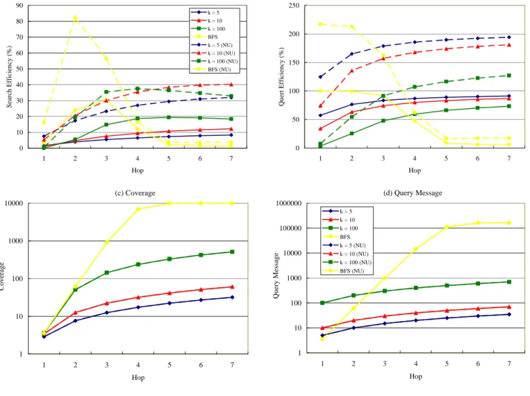
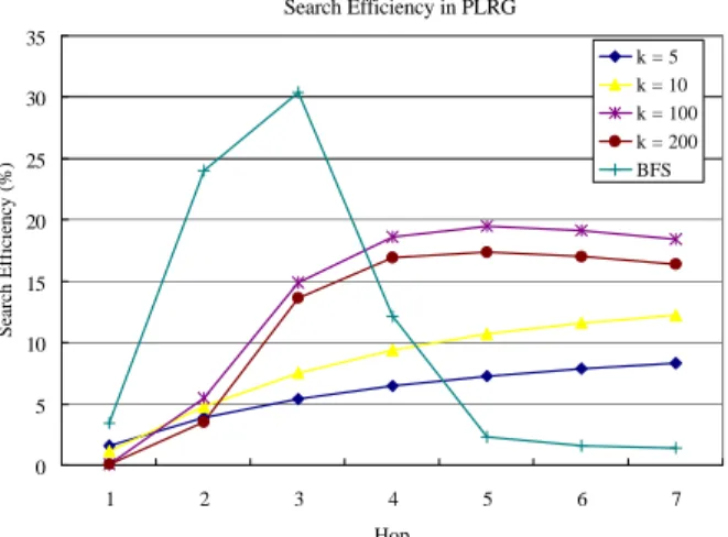
B. Performance Analysis

To analyze the characteristics of dynamic search, we use the knowledge we have learned in previous

sectionswhere we mathematically formulate SE. In this section, we analyze only in the PLRG. The general

form of SE in (26) applies for dynamic search and Ch is given by (23), except eh=1 = f1·G'0(1), e2=h=n =

Fig. 9. Performance comparison by various metrics— (a) Search Efficiency, (b) Query Efficiency, (c) Coverage, and (d) QueryMsg— for RW of various number

of walkers k and for BFS in PLRG with R = 1% under uniform and non-uniform (NU) object distribution. Solid lines represent data of uniform distribution and dashed-lines represent non-uniform distribution.

(

)

1 0 1 1 ( ) ' (1), for 1 1 1 ' (1) , for 2 ( ) 1 1 , for , h h i h h i C h i k i h r P V f p G h f p G h n P R h n − = ⋅ ⋅ =   − −_ ⋅ ⋅ _ ≤ ≤   _{⋅ − −}  _>       ₍₁₄₎ where rh is specified by (12).

As for the parameter design, we refer to the observation in Fig. 6, where BFS performs the best in the first two hops and lower fs for M-BFS achieve more consistent performance in the long-term search. Thus, we design two sets of parameters: the first one, Dynamic-1, performs BFS in the first two hops and random walks in the following phase (n = 2); the second one, Dynamic-2, performs BFS in the first two hops, M-BFS with f = 0.3 at the third hop, and then random walks (n = 3). The number of walkers k in RW

is dynamically determined by the number of outstanding query messages at hop n, i.e. Ch=n. The detailed

parameters are shown in Table II.

We generate SE of Dynamic-1 and -2 and make performance comparison with BFS, M-BFS (f = 0.3), and RW (k = 100) in Fig. 8. We take M-BFS with f = 0.3 in order to compare with Dynamic-2, which uses

f3 = 0.3. And we use 100 as the number of walks for RW since it generates the best performance (in Fig.

7).

(a) Search Efficiency

0 10 20 30 40 50 60 70 80 90 1 2 3 4 5 6 7 Hop Search Efficiency (%) k = 5 k = 10 k = 100 BFS k = 5 (NU) k = 10 (NU) k = 100 (NU) BFS (NU) (b) Query Efficiency 0 50 100 150 200 250 1 2 3 4 5 6 7 Hop Quert Efficiency (%) (c) Coverage 1 10 100 1000 10000 1 2 3 4 5 6 7 Hop Coverage (d) Query Message 1 10 100 1000 10000 100000 1000000 1 2 3 4 5 6 7 Hop Query Message k = 5 k = 10 k = 100 BFS k = 5 (NU) k = 10 (NU) k = 100 (NU) BFS (NU)

In Fig. 8, we can observe that dynamic searches outperform other algorithms especially in the long-term search. They resemble BFS within h=2 as expected and perform consistently as random walk does, thus outperforming others in long-term search as we design. Note that Dynamic-2 trades its performance at h = 3 for its long-term efficiency by using a low probability f = 0.3, and vice versa for Dynamic-1.

NON-UNIFORM OBJECT DISTRIBUTION

Throughout our analysis, for simplicity we had assumed the object distribution as uniform. However, this assumption leads to the conclusion that QueryHits equals to R·Coverage, which violates our argument in Section II.A that Coverage is only one of the conditions to produce QueryHits. To support our argument and justify our consideration of QueryHits in SE rather Coverage, we analyze SE under a non-uniform object distribution as proposed in [11].

In this object distribution, the probability a search agent (vertex) owns certain object is proportional to its degree d. Let O be the event that certain search agent owns the targeted object, then the probability agent i has the object is determined by

1 ( ) i , i i _N j j R N d P O d d = ⋅ ⋅ ∝ = ∑ (15)

such that ?iPi(O) = R·N, the total number of objects distributed in the network, where di = m / i

1/t [4].

Analytic Derivation:

Since the object distribution is not uniform, we cannot simply use R·Coverage to represent QueryHits, which in fact is formulated by

1 1 1 1 ( ) ( ) ( ), for 1 1 ( ) ( ) ( ) ( ), for 2, N i i h i h N i i j i i h i j QueryHits h P O P V h P O P V P O P V h = − = =  ⋅ =   =   _{ − ⋅ ≥}    

∑

∑ ∏

(16)

where Pi(Vh) is given by (5) and Pi(O) by (15).

For SuccessRate, we generalize the form 1- (1- R)C in (4) for the uniform distribution to deliver the one

in non-uniform distribution: 1 1 1 1 ( ) ( ) . N h i i j i j SuccessRate P O P V = =   = −

∏ ∏

_ − _ (17)

Now, equations (16), (17), and (6) suffice to solve SE defined by (2) for BFS.

For RW, QueryHits(h) follows formula (16) derived in BFS and SuccessRate follows (17) in BFS, where

Pi(Vh) is given by (13) and Pi(O) by (15).

Search Efficiency Analysis:

We plot analytic data in Fig. 9, where the dashed-lines represent the data under non-uniform (NU) object distribution. We use the same colors to represent searches with identical parameters. We find that SE in Fig. 9(a) is significantly increased under NU distribution for both BFS and RW. The performance increase is around 75% ~ 250% for RW at h = 7 and 250% for BFS at h = 2. This can be explained by the graph property that vertices tend to connect to those with higher degrees [1, 2], which has been validated by simulations in [11].

Metrics Analysis:

Fig. 9(c) indicates that every search in question generates identical Coverage under different object distributions, and Fig. 9(d) draws the same

conclusion for QueryMsg. Therefore, these two metrics totally fail to distinguish the performance variance under NU distribution. Moreover, in Fig. 9(b), Query Efficiency, defined by QueryHits/(QueryMsg? R), explains the performance increase by indicating more QueryHits found given that same number of QueryMsg. In consequence, SE, in which

QE is a critical element, well characterizes the performance difference in the two

結論與建議

In this project we define a unified metric, Search Efficiency (SE),

addressing performance in searching networks in terms of Query Efficiency,

responsiveness, and reliability. Mathematical formulas and approximations of

SE and other existing metrics are derived to characterize performance and

provide in-depth analysis for various search algorithms. We justify the

correctness of SE in performance evaluation by analyzing it in an ideal topology,

strictly binary tree. We further demonstrate its ability to characterize search

performance in a large-scale PLRG, the real-world network topology.

We conclude that existing metrics either leads to biased conclusions

regarding performance or fail to reflect performance variance when network

conditions change. Moreover, they tend to provide wrong guidelines for the

design of various algorithm parameters (e.g. TTL, k, and f). The proposed metric,

SE, effectively characterizes the performance variance under different network

conditions and delivers objective and in-depth performance analysis.

In the final analysis, the outstanding performance of dynamic search, the

new algorithm devised based on the guidance of SE, manifests the efficacy of

SE to conduct design of search algorithms. Therefore, our proposal of SE

參考文獻

[1]

M. E. J. Newman, S. H. Strogatz, and D. J. Watts. Random graphs with arbitrary degree

distribution and their applications. Phys. Rev. E, 64:026118, 2001.

[2]

L. A. Adamic, R. M. Lukose, A. R. Puniyani, and B. A. Huberman. Search in power-law

networks. Phys. Rev. E, 64:046135, 2001.

[3]

L. A. Adamic. The small world web. Proceedings of the 3

rd

European Conf. on Digital

Libraries, volume 1696 of Lecture notes in Computer Science, pages 443-452. Springer,

1999.

[4]

W. Aiello, F. Chung, and L. Lu. A random graph model for massive graphs. Proceedings of

the thirty-second annual ACM symposium on Theory of Computing, pages 171-180, 2000.

[5]

Q. Lv, P. Cao, E. Cohen, K. Li and S. Shenker. Search and replication in unstructured

peer-to-peer networks. ICS, June 2002.

[6]

B. Yang and H. Garcia-Molina. Improving Search in Peer-to-Peer Networks. ICDCS, July

2002.

[7]

D. Tsoumakos and N. Roussopoulos. Adaptive Probabilistic Search (APS) for Peer-to-Peer

Networks. Technical Report CS-TR-4451, Un. of Maryland, 2003.

[8]

S. Milgram, The small-world problem. Psychology Today, 1:62-67, 1967.

[9]

S. Jiang, L. Guo and X. Zhang. LightFlood: an Efficient Flooding Scheme for File Search in

Unstructured Peer-to-Peer Systems. ICPP, Oct. 2003.

[10]

B. F. Cooper and H. Garcia-Molina. SIL: Modeling and measuring scalable peer-to-peer

search networks. International Workshop on Databases, Information Systems and

Peer-to-Peer Computing, Berlin, 2003.

[11]

T. Lin, H. Wang, and J. Wang. Search Performance Analysis and Robust Search Algorithm in

Unstructured Peer-to-Peer Networks. CCGrid, April 2004.

[12]

C. Gkantsidis, M. Mihail, and A. Saberi. Random walks in peer-to-peer networks. Infocom,

March 2004.

[13]

I. Stoica, R. Morris, D. Karger, F. Kaashoek, and H. Balakrishnan. Chord: A scalable

peer-to-peer lookup service for internet applications. SIGCOMM, 2001.

[14]

V. Kalogeraki, D. Gunopulos and D. Zeinalipour-Yazti, A Local Search Mechanism for

附錄

Hsinping Wand and Tsungnan Lin, “On Efficiency in Searching Networks,”

Infocom 2005.

On Efficiency in Searching Networks

Hsinping Wang and Tsungnan Lin

Graduate Institute of Communication Engineering National Taiwan University

Taipei, 10617 Taiwan {hpwang, tsungnan}@ntu.edu.tw

Abstract-This paper deliberates on various critical aspects

in evaluating searching networks. Existing metrics either draw biased conclusions regarding search performance or provide wrong guidelines for algorithm design. We, therefore, define a unified criterion, Search Efficiency (SE), to objectively address search performance in a comprehensive manner. The goal of

SE is to better characterize performance of searching networks

than existing metrics do as well as to guide the design of future ones. We first validate the correctness of SE in performance evaluation in an ideal graph, strictly binary tree, by analyzing

SE for two typical search methods, breadth first search and

random walk. We further show its strength in performance characterization in the real-world topology, power-law random graph, under various network conditions. We finally design an algorithm, dynamic search, based on SE analysis. Its proved outstanding performance demonstrates the strength of SE to provide guidance for the future design of searching networks.

Index terms— Combinatorics, Graph theory, Deterministic

network calculus

I. INTRODUCTION

Searching networks, including social networks and computer networks, play an increasingly important role in human activity. A significant example is the recently popular peer-to-peer (P2P) file-sharing systems, e.g. Gnutella and KaZaA, where every peer collaboratively forms a searching network to locate desired files by a real-time search. In the social context of searching networks, people search their acquaintances for a particular item or expertise in a specific domain. Their acquaintances in turn report whether they have the desired item (expertise) or subsequently deliver this query to their next-step acquaintances. In this fashion, a

social searching network or so called human

acquaintanceship graph [8] is formed. Thus, a searching

network is a system where each participant contributes to the network and collaborates to help others search targeted resources.

In a searching network, one of the critical issues is to maximize search performance by choosing or designing algorithms used to perform the search process. Novel algorithms [5, 6, 7] have been proposed to address different search aspects, such as success rate, search cost, coverage, or number of hits, but an objective and comprehensive evaluation metric is missing. As a result, these algorithms tend to be designed with biased considerations and evaluated in limited dimensions.

Breadth-first search (BFS) and random walk (RW) [5] are

two basic and typical search methods in searching networks. BFS inherently maximizes the search speed and coverage but risks generating search queries in an uncontrolled (exponential) manner. RW, on the other hand, minimizes search cost but generates limited search coverage and results. As a result, one might draw distinct conclusions about algorithm performance, if different metrics are concerned. For example, Gkantsidis et al. [12] claimed RW performs better than BFS in terms of number of hits and failure probability give the same search cost for BFS and RW, but implicitly assumed an infinite search time for RW, which is clearly unfair. Jiang et al. [9] evaluated their proposed search scheme only by search coverage and message cost, leaving search speed and success rate unchecked. Lv et al. [5] provided a spectrum of aspects on evaluation, but analyzed them individually and still lacked an overall consideration.

Our work, therefore, deals with these one-sided perspectives and synthesizes a unified search criterion,

Search Efficiency (Section II), which is critical particularly

in P2P endeavors, to objectively evaluate search algorithms and provide overall guidance for the design of searching networks.

With the unified metric SE, we first validate its correctness by deriving its mathematic formulas for BFS and RW in a simple topology, strictly binary tree (SBT), and analyzing whether the performance indicated by SE is reasonable. Furthermore, we extend the results of Newman [1] and Adamic [2] and further consider “redundancy” to analytically approximate SE for BFS, M-BFS [14], and RW in a power-law random graph (PLRG), which is shown to be the real topology of current searching networks. We thus validate SE in comparison with previous simulation works [5, 9, 11], deliver the unique performance characterization of SE, and provide in-depth analysis.

Throughout the analysis in this paper, we compare various existing metrics with SE to address their limitation and strength. We show that no matter in SBT or PLRG, existing metrics draw biased conclusions regarding search performance; they either provide one-sided considerations or deliver wrong guidelines for algorithm design. Moreover, they fail to characterize performance variance under distinct network conditions, such as object replication ratios (Section III) and object distributions (Section VI).

In the final analysis, we propose a new algorithm,

dynamic search, based on the results of SE analysis. We

prove this algorithm outperforms existing ones and SE effectively provides guidance for algorithm design.

This work was supported in part by National Science Council under grant 93-2213-E-002-057, and by Quanta Computer Inc. under grant 092E0048.

In summary, our contributions are stated as follows: • We propose a unified and objective metric, Search

Efficiency, for evaluating searching networks and

characterizing search algorithms.

• We mathematically analyze critical performance metrics— search coverage, cost, success rate, number of hits, and SE— in searching networks.

• We analytically evaluate various algorithms, including BFS, M-BFS, RW, and a novel search, in SBT and PLRG, under uniform and non-uniform object distributions.

• We devise a new search algorithm, dynamic search, based on the knowledge from temporal SE analysis. It is shown to outperform other existing ones, thus SE proved to provide solid guidance for algorithm design. This rest of this paper first follows with the definition and explanation of Search Efficiency in Section II. We then analytically derive the general form of SE and provide in-depth discussion on the performance of BFS and RW in SBT in Section III and PLRG in Section IV. Section V presents the novel algorithm, dynamic search. We analyze algorithms under non-uniform object distribution in Section VI, then finally conclude in Section VII.

II. SEARCH EFFICIENCY

We argue that to best characterize the efficiency of any system is to measure its ability to transfer its input to generate meaningful output, which is applicable in the evaluation of search methods performed in any network. In a social network, the input of a search largely involves the cost required for querying process including costs of phone calls, transportation, and even consulting. As for output, it should be measured by searchers’ satisfaction in terms of the chance of success, the response speed, and quality of responsive results. To clarify the definitions of and relations between these inputs and outputs in the context of searching networks, we start a series of discussions about Search

Efficiency with Query Efficiency (QE). A. Query Efficiency

In general, the most critical aspects of search performance involve the extent of search coverage (output) [2] and the cost required to cover the network (input) [5]. By search coverage, denoted as Coverage or C, we mean the number of distinct or effective peers visited by search queries, i.e. we do not count the repeatedly visited ones. In addition, by cost, denoted by QueryMsg, we mean the number of queries incurred, for it is a representative factor to which other cost factors (e.g. computer processing power or costs for phone calls and transportation) tend to be proportional. Thus it is trivial to say a search which uses S query messages to traverse distinct S nodes is perfectly or 100% efficient in terms of query generation. Additionally, we can define a sort of efficiency as

Coverage / QueryMsg. However, the end goal of

searching is not to cover as many nodes in the network as possible. Rather, its ultimate goal is to search out the

desired targets or objects, in which covering is only one of the adequate conditions (e.g. cache or previous experience) for that end. This is true when the searching network is well-designed, e.g. Chord [13], such that large search coverage is not necessary, or when object distribution is not uniform in which directed search is preferred. We will show performance difference between Coverage and QueryHits under non-uniform object distribution in Section VI.

Thus, we define QueryHits(t) as the number of desired objects found “at” search time t, which is measured by the number of hops or depths, to quantify the yields of a search. We introduce the factor search time t for the purpose of future discussion. Again, we

might define the efficiency of queries as

?tQueryHits(t)/QueryMsg. However, this definition is

sensitive to the population of desired objects, which is irrelevant to the performance of search algorithms themselves and should be factored out. For this purpose, we introduce the notion of object replication ratio R defined as the ratio of the number of targeted objects to the network size (N). To cancel the population factor out, we normalize it with respect to R and thus formulate Query Efficiency (QE) as

1 ( ) 100% (%) , TTL t QueryHits t Query Efficiency QueryMsg R = = ∑ × (1)

where TTL refers to the termination condition of searches, measured in hops. To exemplify, we suppose a search consuming 100 messages to find 1 targeted object in a network with R of 1%, which reveals that

1% of nodes have the desired object. By (1), QE =

100% and we thus call it a perfectly query-efficient search. Furthermore, if the objects are uniformly distributed in the network, we can reasonably claim that the search effectively covers 100 nodes (from 1/1% = 100) and this provides a clear view of the perfect efficiency.

B. Responsiveness

One of the goals of searching, as addressed previously, is to find out possible objects while the other is to find them as soon as possible. We define search response time, denoted by t, measured by discrete numbers of hops, to evaluate the speed of searching objects, or responsiveness of a search. If a search finds Q desired objects in its hth step or in its

hth-nearest acquaintances, we denote it as

QueryHits(t=h)=Q.

We argue that a search getting hits in a faster fashion delivers better users’ experience and should be gauged as higher reputation. More specifically, responsiveness of a search should be inversely proportional to the response time t. To consider this factor for SE, we may simply divide QE by the weighted response time,

which is computed by ?t[t·QueryHits(t)] /

?tQueryHits(t). However, this method would generate

uses 1000 messages to get 99 hits at t = 1 and 1 hit at t = 100 with R = 10%, resulting in a weighted response time of (1·99+100·1)/100 or 1.99. According to QE in (1), if we don’t count the hit at t = 100, the search is 99% query efficient, but it dramatically reduces to 50.25% efficiency due to dividing by response time 1.99 when that hit is calculated. This method unreasonably emphasizes the slow search hit. We argue that any query hits contribute positively to the search itself despite long response time. We thus aggregate these responsive hits rather than divide by the averaged response time to give efficiency as

1 ( ) / 100% TTL t QueryHits t t QueryMsg R = _× ∑ .

The efficiency of this example becomes 99.01% rather than 50.25%, where the last found hit contributes 0.01% to efficiency, rather than severely reducing it.

C. Reliability

The last concern is reliability, which is measured by

SuccessRate in our design of SE. We introduce it so as

to further consider the satisfaction of user experience. Consider two searches (A and B), each performing two runs, as shown in Table I. We assume all objects are found at the same response time. The success rate of Search A is 50% while B is 100%.

TABLE I

SEARCH DATA FOR ILLUSTRATING SUCCESSRATE

Search A Search B

QueryMsg QueryHits QueryMsg QueryHits

Run1 100 2 100 1

Run2 100 0 100 1

Note that if we compute efficiency without

SuccessRate, we will gain the same result for Search A

and B. However, one of the runs in Search A (Run 2) fails and thereby we neglect to measure the penalty of user experience in Run 2. By introducing the term

SuccessRate, SE of Search B remains the same, but SE

of A is halved. In this manner, it successfully addresses the user satisfaction level while the two searches get the same number of hits at the same message costs. In sum, the term SuccessRate is aimed to successfully measure the satisfaction level from users’ perspective. Finally, we define the overall criterion for evaluating searching by 1 ( ) TTL t QueryHits t t SuccessRate Search Efficiency QueryMsg R = =∑ × ,(2)

where TTL stands for the limit of search covering.

D. Limitations of Search Efficiency

The design goal of SE is to capture a simple but representative view of search performance. As a result, it is possible to consider more complex considerations for search evaluation. We list three possible aspects that are not covered by SE:

1) In the context of computer searching networks, the implementation of caches or DHT would significantly improve the search performance, which

SE could reflect. However, SE doesn’t consider the

additional resources (processing power or memory) required by performance-boosted mechanisms, such as

hash functions or caches, thus potentially

overestimating the efficiency of algorithms adopting these additional mechanisms.

2) The costs of searching each computer or peer should not be equally weighted. Consulting an institution for recommendations is clearly more costly than asking a close friend, although we only assume they are equally costly.

3) We make a limited measure of responsiveness by the factor t. For instance, it would be more flexible using ta, a > 0, to adjust the extent to which search responsiveness is concerned.

By means of Search Efficiency, we can objectively evaluate performance of algorithms in searching networks. In the remaining of this paper, therefore, we aim to characterize various existing search algorithms in terms of SE and demonstrate the biased view of existing search metrics compared with SE. In the following sections, we will mathematically derive the formulas for SE in the context of three basic search approaches, BFS, RW and M-BFS, the variation of BFS, in two representative topologies, the strictly binary tree (SBT) as well as the power-law random graph (PLRG), in order to demonstrate the strength of

SE.

IV. STRICTLY BINARY TREE

We assume an N-vertex strictly binary tree whose depth is about log2N and that the requester is at the root such that the response time (t) of a query hit is the same as the depth (d) where the target object is located. This tree is shown in Fig. 1. Moreover, for simplicity of analysis, we assume objects are uniformly distributed in the tree or graph until Section VI.

Before analyzing specific algorithms, we first prepare two common factors for the derivation. Firstly, the number of objects searched out (QueryHits) is proportional to the search coverage C. Thus, we have

QueryHits= ×R C. (3) ...

Fig. 1. A strictly binary tree with the requester at the root Depth 2

Depth 3 Depth 1

Fig. 2. Search Efficiency for BFS terminated by incremental TTLs (Depth) in a strictly binary tree with various replication ratios R

Secondly, the success rate of a search is also relevant to the search coverage. To begin with, we know that each node owns the target object with a probability of

R; that is, each node lacks the object with a probability

of 1- R. Suppose a search covers C vertices and thus the probability these C nodes share no targeted object

is (1- R)C. Inversely, the probability these C nodes

share one or more objects, or equivalently SuccessRate, is determined by

1 (1 )C

SuccessRate= − −R . (4)

A. Breadth First Search in Strictly Binary Tree (SBT)

Analytic Derivation: Breadth-first search (BFS)

performs by broadcasting the received queries to all neighbors except where the received query came from. Therefore, by the regular structure of a strictly binary tree, the search coverage terminated at depth TTL is given by

1

( ) TTL_t 2t

Coverage C =∑₌ (5) Furthermore, the number of messages required to traverse the tree is the same as the quantity of its search coverage due to the very nature of BFS. Thus,

QueryMsg = C = ?t 2 t . According to (1), (3), and (5), we attain 1 1 2 100% 100% 2 t TTL t BFS TTL t t R QueryEfficieny R = = ⋅ = ∑ × = ∑ (6)

Surprisingly, the formula of QEBFS yields a constant,

1 or 100%, regardless of the replication ratio R or the termination depth TTL. By the definition of QE, this means that BFS is a perfectly query-efficient search in the context of a binary tree; that is, BFS generates no redundant messages while traversing a binary tree. The idea of redundancy will be further defined and discussed in the next section.

Finally, the general formula of SE defined in (2) for BFS in a binary tree is

(

)

12 1 1 2 1 1 . 2 t TTL t t TTL t BFS _{TTL t} t t SE = R ∑= =   = × − −_{ }   ∑ ∑ (7)

The derived SEBFS is complex for one to gain insight

of its properties due to the running variable t and various possible values of R. To deliver a clearer understanding, we assume the replication ratio R << 1, which is true in real searching networks, and

approximate (7) as

(

)

[

]

∑ ∑ ∑ = = = = _{× − − ⋅∑ = ⋅} ≅ TTL t t TTL t t TTL t t TTL t t BFS R R t t SE _{1 1} 1 1 _{1 1 2 2} 2 2 .(8)

Search Efficiency Analysis: To exemplify SEBFS, we

set R = 0.1% (far less than 1) and obtain by (8) SETTL=1

= 0.2%, SETTL=2 = 0.4%, and SETTL=3 = 0.67%. Note SE

is strictly increasing with respect to TTL— SETTL=2 is

exactly twice of SETTL=1 and SETTL=3 is more than three

times of SETTL=1. The reasons are two-fold. Firstly, as

formula (6) shows, BFS in a binary tree is perfectly

query-efficient, which means every query positively contributes to its search coverage and in turn produces promising increase in SE. Secondly, the speed at which query hits are returned is faster than the decay factor of

response time t. Furthermore, formula (8) tells that the

benefits from BFS are increasingly proportionally to 2t

while the factor t is used to compensate the demerit of

long search time, where the factor 2t tends to dominate.

Thus we conclude every query or every additional covered depth makes a positive contribution to the overall performance despite the compensation of time, given that the replication ratio is much smaller than unity.

We present analytically-derived data of SEBFS,

without approximation, by (7) with a spectrum of

parameters, Rs and TTLs, in Fig. 2. Firstly, we note that

SEBFS for all Rs approaches some fixed level in the

long run. This fixed level, obtained by (7) for large t, is determined by the characteristic of the searched topology— strictly binary tree— that is irrelevant to R. Second, the short-term increase of SE for high R (10% or 5%) results from the perfect query efficiency and popularly distributed objects, while the long-term decrease is due to the compensator of response time t.

If we use the notion ta suggested in Section II.D, where

a is 0 or small for some application scenarios and

responsiveness is of little concern, SE in (7) will

increasingly grow to some fixed level. Third, as for low R (0.1% or 0.5%), the results in Fig. 2 are reflective of the discussions in the above paragraph— SE is consistently increasing.

Note that, however, if we take TTL as infinity in (7),

it gives zero seemingly contradicting our notion. In reality, however, TTL cannot be infinity but is generally 7~10, in which SE still generates a fixed level of performance reflecting the characteristics of SBT.

Search Efficiency for BFS

0 5 10 15 20 25 30 35 40 1 2 3 4 5 6 7 8 9 10 Depth Search Efficiency (%) R=10% R=5% R=1% R=0.5% R=0.1%

Fig. 3. Performance comparison by various metrics— (a) Search Efficiency, (b) SuccessRate, (c) Coverage, and (d) QueryMsg— for RW of various number of walkers k and for BFS in a strictly binary tree with R = 1%

Metrics Analysis: We compare two metrics, SE and

Coverage in this scenario. The results of Coverage of

BFS can be referred to in Fig. 3(c). If we take only

Coverage (C) into consideration, it produces the same

performance in spite of different extents of object

replication (different values of R) since C by (5) is

independent of R. Hence, Coverage fails to characterize the performance variance in searching networks with different replication ratios. On top of this, if the design goal is to maximize C, then one may conclude that the choice of termination condition TTL is the larger the better— an impractical conclusion. On the other hand, if we only inspect QueryMsg, we will get entirely opposite conclusions. Therefore, Coverage and QueryMsg draw contradictory conclusions and fail to provide comprehensive guidance.

In fact, by the indication of SE in Fig. 2, TTL should be small when R is large in order to avoid unnecessary message propagation when R is large and to generate satisfactory results when R is small. In sum, SE better characterizes performance and provides a better guideline of TTL design than Coverage and QueryMsg.

B. Multiple Random Walks in Strictly Binary Tree

When it comes to RW search, we use multiple “walkers” to traverse the network and the number of

walkers is denoted by k. Each walker independently searches the network and randomly chooses one of the next-hop neighbors to continue its journey to the limit of TTL hops.

Analytic Derivation: To begin with, we consider

Coverage to derive SE. We know each vertex at depth t

is visited by a random walker with equal probability,

1/2t. Moreover, each random walker independently

makes its own decisions to traverse the topology. Thus, the probability that all k walkers don’t visit a certain vertex is (1- 1/2t)k. As a result, at depth t, the average number of nodes visited (Coverage per Depth) by k random walkers is given by the expectation

1 ( ) 2 1 (1 ) 2 t k t t E X = _ − − _  . (9)

By (3), QueryHits(t) = R·E(X)t. Moreover, the query

messages of random walk are generated per hop for each walker until terminated by the TTL limit, hence

QueryMsg = k·TTL. (10)

As a result, QE of k-random walk is

1 ( ) 1 ( ) TTL TTL t t t t RW k R E X E X QE k TTL R k TTL = = = ⋅ = = ⋅ ⋅ ⋅ ∑ ∑ _{. (11)}

Furthermore, from (4), we obtain

1 ( )

1 (1 )C 1 (1 ) TTLt E X t. SuccessRate_{= − −}R _{= − −}R ∑= ₍₁₂₎

Therefore, Search Efficiency for k-random walks is (a) Search Efficiency

0 2 4 6 8 10 12 14 16 18 1 2 3 4 5 6 7 8 9 10 Depth Search Efficiency (%) k=2 k=5 k=20 k=50 BFS (b) Success Rate 1 10 100 1 2 3 4 5 6 7 8 9 10 Depth Success Rate (%) k=2 k=5 k=20 k=50 BFS (c) Coverage 1 10 100 1000 10000 1 2 3 4 5 6 7 8 9 10 Depth Coverage k=2 k=5 k=20 k=50 BFS (d) QueryMsg 1 10 100 1000 10000 1 2 3 4 5 6 7 8 9 10 Depth QueryMsg k=2 k=5 k=20 k=50 BFS