1636 OPTICS LETTERS / Vol. 22, No. 21 / November 1, 1997
Four-wave mixing between a soliton and noise
in a system with large amplifier spacing
Sien Chi and Chuan-Yuan Kao
Institute of Electro-Optical Engineering, National Chiao Tung University, Hsinchu 30050, Taiwan, China Senfar Wen
Department of Electrical Engineering, Chung-Hua Polytechnic Institute, Hsinchu 30067, Taiwan, China
Received June 3, 1997
Depletion of soliton energy by four-wave mixing between a soliton and amplifier noise in a system with 100-km amplifier spacing is studied. Dispersion exponentially decreasing fiber is used as transmission fiber. Improvement of the system by the use of a sliding-frequency filter to reduce noise power and the depletion of soliton energy is shown. The system can be further improved by compensation for depleted soliton energy.
1997 Optical Society of America
The amplif ier spacing of a soliton-transmission sys-tem is limited by soliton stability and noise-induced timing jitter.1,2
These limits require that the ampli-fier spacing be much shorter than the soliton period to maintain stable soliton transmission. For large ampli-fier spacing the noise power introduced by the optical amplifier is significant. Therefore amplif ier spacing shorter than,50 km is usually used in a soliton sys-tem. For undersea optical cable systems, larger ampli-fier spacing is desirable. In this Letter we consider a soliton system with 100-km amplif ier spacing, in which dispersion exponentially decreasing fiber3
(DEDF) is used as the transmission medium and a Fabry– Perot filter (FPF) is used as the in-line f ilter to reduce tim-ing jitter.4 As a fundamental soliton is maintained along the DEDF, the stability condition is satisf ied by use of DEDF. The in-line filter stabilizes the carrier frequency of the soliton and reduces timing jitter. It was found that there is significant four-wave mixing (FWM) between soliton and amplifier noise in such a system because of high noise power and phase match-ing. The soliton-noise FWM depletes the soliton en-ergy, and the soliton broadens. The improvement of the system by the use of a sliding-frequency f ilter5 (SFF) to reduce noise power and the depletion of soli-ton energy is considered. In addition, the system can be further improved by compensation for the depleted soliton energy.
The pulse propagation in a DEDF can be described by the modified nonlinear Schr¨odinger equation i≠U ≠z 2 1 2 b2szd ≠2U ≠t2 2 i 1 6 b3 ≠3U ≠t3 1 gjU j 2 U 21 2 iaU . (1) In Eq. (1), U is the normalized field envelope; b2szd
exps2azdb2s0d is the second-order dispersion, where
b2s0d is the initial value at every amplification stage;
b3is the third-order dispersion; g n2v0ycAeff, where
n2 is the Kerr coeff icient, v0 is the carrier frequency,
c is the velocity of the light in vacuum, and Aeff is
the effective fiber cross section; a is the f iber loss. For the numerical calculations, the carrier wavelength is taken to be 1.55 mm and the other parameters are taken to be b3 0.14 ps3ykm, n2 3.2 3 10220m2yW,
Aeff 50 mm2, and a 0.2 dBykm. A FPF is inserted
after every amplif ier. We choose the bandwidth of the filter to be Dnf 10Dns, where the soliton spectral
width is Dns 0.314ytw and tw is the soliton pulse
width (FWHM). We take tw 10 ps and tw 20 ps
as examples to show the results.
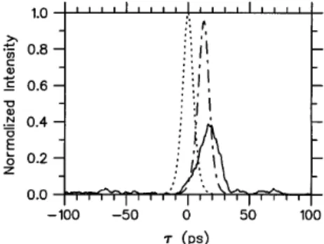
Figure 1 shows the input 10-ps soliton and the pulse shape of the soliton after propagating 10,000 km along the DEDF with b2s0d 20.5 ps2ykm, where the gain
of every amplifier is expsaLad and the amplifier
spac-ing is La 100 km. The spontaneous-emission
fac-tor of the amplif ier is nsp 1.2. An in-line filter of
314-GHz bandwidth is used. The pulse shape of the soliton after propagating 10,000 km without amplifier noise being considered is also shown for comparison. One can see that soliton energy is significantly de-pleted by the interaction with amplifier noise. The
Fig. 1. Pulse shape of a 10-ps soliton after propagating 10,000 km along DEDF with b2s0d 20.5 ps2ykm (solid curve). The amplif ier spacing is 100 km. An in-line f ilter with a 314-GHz bandwidth is used. The pulse shape of the input soliton is shown by the dotted curve. The pulse shape of the soliton after propagating 10,000 km without amplif ier noise being considered is shown by the dashed – dotted curve.
November 1, 1997 / Vol. 22, No. 21 / OPTICS LETTERS 1637 interaction is due to the FWM between soliton and
noise. The soliton-noise FWM is eff icient because the noise power is high and the f iber dispersion is low in the considered DEDF. The asymmetric distortion of pulse shape is due mainly to the third-order fiber dis-persion and the disdis-persion introduced by in-line f il-ters. To estimate the soliton energy, we f irst f ilter the soliton with an ideal bandpass filter of bandwidth Dnw 4Dns. Then the soliton energy is calculated
within a window of Dtw 4Dts in the time domain,
and the calculated energy is denoted as Es. We
simu-late the transmission of a single soliton 16 times to ob-tain the average value of the soliton energy, ¯Es. The
ratio of the energy depletion is def ined as
rd 1 2 ¯EsyEs0, (2)
where Es0 is the initial value of the soliton energy.
Figure 2 shows the energy-depletion ratio rdalong the
fiber for the case shown in Fig. 1. The ratio rn EnyEs0 is also shown in Fig. 2, where En nspsG 2
1dhnDnwDtwzyLa is the accumulated noise energy
without nonlinear mixing and z is the transmission distance. One can see that the noise energy from the optical amplifiers is small compared with the soliton energy, but the depletion of soliton energy owing to soliton-noise FWM is signif icant. From Fig. 2 one can see that rd increases almost linearly with distance.
At the end of 10,000-km transmission, ¯Es is only two
thirds of Es0. The energy depletion manifests the
pulse distortion shown in Fig. 1.
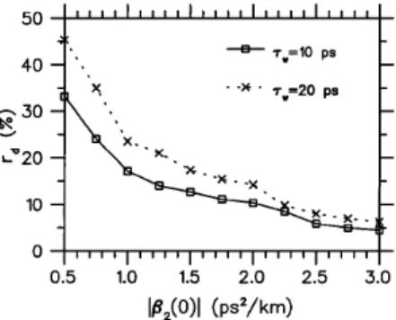
Figure 3 shows the depletion ratio rd with respect
to jb2s0dj for 10- and 20-ps solitons after the
10,000-km transmission distance. One can see that rd can
be reduced by the use of higher f iber dispersion. FWM is efficient when the soliton spectrum is near dispersion frequency. The deviation of the zero-dispersion frequency from the carrier frequency of the soliton is jb2szdjyb3. Within an amplif ier spacing, as
jb2szdj decreases with distance the zero-dispersion
fre-quency moves toward the soliton frefre-quency. There-fore soliton-noise FWM increases with distance within an amplif ier spacing. The smallest f iber dispersion is jb2sLadj at the end of every amplifier stage, and the
zero-dispersion frequency lies within the soliton spec-tral width when jb2sLadj % b3pDns. Thus the
cor-responding initial fiber dispersion jb2s0djmin can be
estimated as a lower limit:
jb2s0djmin 0.314pb3expsaLadytw, (3)
where jb2s0djmin 1.38 ps2ykm and jb2s0djmin
0.7ps2ykm for t
w 10 ps and tw 20 ps, respectively.
Both of the depletion-ratio curves in Fig. 3 are almost linear for jb2s0dj above the lower-limit values, and
the slopes increase drastically for jb2s0dj below them.
Although a larger jb2s0dj leads to higher soliton power,
the phase-matching condition is less well satisf ied, and the efficiency of the soliton-noise FWM decreases in the case of the same pulse width. For the same jb2s0dj, the rd of the 10-ps soliton is smaller than the rd of the 20-ps soliton since the former has a larger
signal-to-noise ratio. If the pulse width is too short, the other effects such as third-order dispersion and self-frequency shift may deteriorate the pulse shape.
From Fig. 3, we can see that rd decreases as jb2s0dj
increases and the pulse width decreases. However, in the presence of neighboring solitons, and when noise-induced timing jitters are considered, the system performance may not be improved as jb2s0dj increases
and the pulse width decreases.
To study the performance of the system, we consid-ered the allowed transmission distance of a 10-Gbitys system for a 1029 bit-error rate. We simulated
254 bits to calculate the bit-error rate, where the prob-abilities of 1 and 0 bits were the same. The squares in Figs. 4(a) and 4( b) show the allowed transmission distances versus jb2s0dj for 10-ps and 20-ps solitons,
respectively. It is known that the SFF can effectively reduce noise power and timing jitter.5
Soliton-noise FWM can also be reduced by use of a SFF. The crosses in Figs. 4(a) and 4( b) show the cases in which the SFF was used, where the f ilter is the same as the Fabry – Perot in-line filter used above except that the SFF’s central frequency is upsliding, with rates of 3 and 5 GHzyMm in Figs. 4(a) and 4(b), respectively. One can see that the improvement of the transmission distance ranges from 1000 to 2000 km and that there exists an optimum jb2s0dj for the maximum
transmis-sion distance. When jb2s0dj is small, soliton-noise
FWM is significant. When jb2s0dj is large, although
the energy-depletion ratio is reduced, as shown in Fig. 3, soliton– soliton interaction and noise-induced timing jitter are enhanced and the transmission distance is limited. Comparing Figs. 4(a) and 4( b) shows that, for jb2s0dj , 0.6 ps2ykm, the transmission
Fig. 2. Energy-depletion ratio along the f iber for the case shown in Fig. 1 (solid curve). The dashed line represents the ratio of the accumulated noise energy and initial soliton energy in the absence of Kerr nonlinearity.
Fig. 3. Energy-depletion ratio rd versus initial f iber dis-persion jb2s0dj for both 10- and 20-ps solitons at a 10,000-km transmission distance.
1638 OPTICS LETTERS / Vol. 22, No. 21 / November 1, 1997
Fig. 4. Allowed transmission distance versus initial f iber dispersion jb2s0dj for (a) 10-ps and (b) 20-ps solitons.
Fig. 5. Soliton pulse shape for the same case as in Fig. 1 (solid curve), except that the energy depletion is completely compensated for. Dotted curve, input soliton pulse shape.
distance is longer for the 10-ps pulse width; for jb2s0dj . 0.6 ps2ykm, the transmission distance is
longer with the 20-ps pulse width. Although the energy-depletion ratio decreases with pulse width for the same jb2s0dj as shown in Fig. 3, the noise-induced
timing jitter is enhanced for the soliton with the shorter pulse width. The transmission distance with the shorter pulse width is less than that with the longer pulse width when jb2s0dj is large.
To compensate for the energy depletion, we can increase amplif ier gain to maintain the estimated aver-age soliton energy, ¯Es rcEs0, where rcis the
energy-compensation ratio. As the energy depletion increases with distance owing to greater noise power, the re-quired amplif ier gain also increases with distance. Figure 5 shows the pulse shape of the soliton for the same case as in Fig. 1, except that the energy deple-tion is compensated for and rc 1.0. One can see
that the pulse shape is much better than that with-out the compensation for the energy depletion. How-ever, rc 1.0 may not be the optimal choice because the
generated noise power through soliton-noise FWM in-creases with rc. With the energy-compensation ratio rc adjusted, the maximum transmission distances for
different jb2s0dj when sliding filters are used are shown
in Fig. 4 by the diamonds. For example, the optimal rc for the case with a 10-ps soliton are 0.95, 0.8, and
0.5 for jb2s0dj 0.2 ps2ykm, jb2s0dj 1.0 ps2ykm, and
jb2s0dj 2.0 ps2ykm, respectively. Comparing the
cases without and with energy compensation shown in Fig. 4, we see that the transmission distance can be improved significantly when jb2s0dj is not too large.
When jb2s0dj is large, although the soliton pulse width
is maintained better with energy compensation, the dispersive wave is larger owing to the greater noise power, where part of the noise is converted from soli-tons through soliton-noise FWM. The enhancement of soliton–soliton interaction by the dispersive wave in-creases with jb2s0dj.
In conclusion, we have shown the FWM between soliton and amplif ier noise in a system with large amplifier spacing, in which DEDF is used as trans-mission fiber. When a low-dispersion DEDF is used in such a system, the depletion of soliton energy ow-ing to the soliton-noise FWM is signif icant because of the phase matching. On the other hand, when the higher-disperison DEDF is used, the FWM is reduced, but the noise-induced timing jitter and soliton–soliton interaction increase. Therefore there exists an opti-mum fiber dispersion for the maxiopti-mum transmission distance. The improvement of the soliton system by use of a SFF and compensation for depleted soliton en-ergy were also shown.
This study was partially supported by the National Science Council, Republic of China, under contract NSC 86-2811-E009-002R.
References
1. L. F. Mollenauer, J. P. Gordon, and M. N. Islam, IEEE J. Quantum Electron. QE-22, 157 (1986).
2. J. P. Gordon and H. A. Haus, Opt. Lett. 11, 665 (1986). 3. K. Tajima, Opt. Lett. 12, 54 (1987).
4. A. Mecozzi, J. D. Moores, H. A. Haus, and Y. Lai, Opt. Lett. 16, 1841 (1991).
5. L. F. Mollenauer, J. P. Gordon, and S. G. Evangelides, Opt. Lett. 17, 1575 (1992).