基於標準與特別演繹樣本訊號元素之稀疏訊號處理法於腦電圖中觸發電位與獨立成份訊號之分析

i

國 立 交 通 大 學

網路工程研究所

碩 士 論 文

基於標準與特別演繹樣本訊號元素之稀疏訊號處理法

於腦電圖中觸發電位與獨立成份訊號之分析

Sparse Signal Representation of EEG and ICA Components

Based on Standard and Specially Trained Dictionaries

研 究 生： 邱俊瑋

指導教授： 邵家健

教授

ii

基於標準與特別演繹樣本訊號元素之稀疏訊號處理法

於腦電圖中觸發電位與獨立成份訊號之分析

Sparse Signal Representation of EEG and ICA Components

Based on Standard and Specially Trained Dictionaries

研 究 生：邱俊瑋

Student: Jun-wei Qiu

指導教授：邵家健

Advisor: Dr. John Kar-kin Zao

國 立 交 通 大 學

網 路 工 程 研 究 所

碩 士 論 文

A Thesis

Submitted to Institute of Network Engineering College of Computer Science

National Chiao Tung University in partial Fulfillment of the Requirements

for the Degree of Master

in

Computer Science June 2010

Hsinchu, Taiwan, Republic of China

iii

基於標準與特別演繹樣本訊號元素之稀疏訊號處理法

於腦電圖中觸發電位與獨立成份訊號之分析

學生：邱俊瑋

指導教授： 邵家健 博士

國立交通大學網路工程研究所碩士班

中文論文摘要

本文將著重介紹一個基於 Matching Pursuit ，並配合改進後的 Grassmannian 參數取 樣方式以及自然梯度設計而出的文化基因演算法。

iv

Sparse Signal Representation of EEG and ICA Components

Based on Standard and Specially Trained Dictionaries

Student: Jun-wei Qiu

Advisor: Dr. John Kar-kin Zao

Institute of Network Engineering College of Computer Science National Chiao Tung University

Abstract

A sparse signal has a large portion of its energy contained in a small number of coefficients, which can be represented with number of samples significantly beneath the Nyquist’s criterion. Sparse signal processing is the application of the mathematics of sparse representations in signal processing. This is essential for ubiquitous medicine and healthcare due to the immense amount of data required for each individual patient monitoring.

A representation dictionary for the target signal space with only minimal number of supports is critical to the stability and consistency of the sparse signal processing schema when employing pursuit algorithms. The overcomplete Gabor dictionary, which can be parameterized into time, frequency, scale and phase, is already known to have efficient representation for electroencephalograms (EEGs).

This thesis includes a Memetic Algorithm based on Matching Pursuit for EEG signal decompositions, and an improved parameter sampling and optimization method for the Gabor dictionary based on natural gradient and Grassmannian concepts.

v

Acknowledgement

First appreciation is to my dearest members of the family; their selfless devotion undoubtedly provides the most sincere support during the period of my academic career far away from home, both physical and mental alike.

Secondly, in these days of my research, the instructors –– John Kar-kin Zao and Peng-hua Wang –– always encouraged me to overcome the difficulties which I originally thought to be insurmountable. This research topic is truly a challenge for my study in my college years, especially the part of digital signal processing and high dimensional information geometry, which are entirely whole brand new areas to me since I’ve never taken any related lectures during my college years. Their untiring and earnest advices have guided me through various obstacles. No achievement would have come out without their professional and genuine instructions.

There’s a special thanks to Alvin Chou, his profound knowledge in clinical and biomedical engineering provides the most recent information and related technologies to the research team; his industrious and irreplaceable works have saved us a lot of time getting familiar with the state-of-the-art biomedical analysis tools during the research period.

Finally, I must thank my former roommate Ting-yu, Tse-wei and Sz-Hsien; the members of the softball team such as Yun-Hsiu, Shu-hua, Tz-Chaio and Zhe-wei. Those who stand with me and share my emotion just like my brothers should take the final prize. It’s really a pleasure to have these valuable companions in such a fascinating and colorful journey.

Jun'wei Qiu

vi

Table of Contents

List of Figures ... viii

List of Tables ... x

Chapter 1. Introduction ... 1

1.1. Motivation ... 1

1.2. Recent Difficulties and Solutions ... 1

1.3. Objectives ... 2

1.4. Research Approach ... 2

1.5. Contributions ... 3

1.6. Thesis Outline ... 4

Chapter 2. Backgrounds ... 5

2.1. Gabor Atoms and Dictionary ... 5

2.2. Matching Pursuit ... 6

2.3. Localized Optimization Methods ... 9

2.4. Grassmannian Frame ... 10

2.5. Memetic Algorithms ... 14

Chapter 3. CMA-ES Based Local Search ... 16

3.1. Identifying the Quasi Sparse Property of EEG Signals, ... 16

3.2. Sparse Representation over Standard Dictionaries ... 17

3.3. Signal Decomposition ... 20

3.4. Matching Pursuit Based on CMA-ES ... 23

3.5. Discovery of Inconsistency ... 23

3.6. Consistency Conditions ... 25

3.7. Experiments ... 27

Chapter 4. Natural Gradient Search over Riemannian Space ... 37

4.1. Geometry of the Gabor Parameter Space ... 37

4.2. Uniform Sampling on Gabor Parameter Space ... 37

4.3. Summary ... 50

vii

5.1. Memetic Concept... 51

5.2. Grassmannian Dictionary Initialization ... 51

5.3. Natural Gradient Optimization ... 53

5.4. Realisation: HyMN-G ... 55

5.5. Comparison with Previous Algorithms ... 56

5.6. Large Scale Analysis on Channel and ICA Signals ... 58

Chapter 6. Dictionary Evolved Based on Training Signal Examples ... 63

6.1. Training Method ... 63 6.2. Decomposition Problems ... 63 6.3. Consistency Conditions ... 64 6.4. Experiment ... 65 Chapter 7. Conclusion ... 69 7.1. Achievements ... 69 7.2. Future Works ... 71 Mathematical Notations ... 72 References ... 73

viii

List of Figures

Figure 1 Gabor Atoms as Shifted and Modulated Gaussian Functions ... 6

Figure 2 Supports of Energy Spreading of a Constant-Scale Gabor System Generated with a Hexagonal Lattice, Fig. 4 (b) of [24] ... 13

Figure 3 Relative Density Map of Time-Frequency Centre of Gabor Atoms ... 16

Figure 4 Gabor and Chirplet Atoms ... 18

Figure 5 Morlet and Mexican Hat Atoms ... 19

Figure 6 Cubic Cardinal B-Spline Atom ... 20

Figure 7 Illustration of Noisy Sparse Single-Trial Signal Decomposition Problem ... 21

Figure 8 Example of Two Almost Identical Atoms with Different Parameters... 24

Figure 9 Comparison of Convergence Rate of Different Dictionaries over ICA Component #20 ... 30

Figure 10 Gabor Energy Map (ICA #20) ... 30

Figure 11 Chirplet Energy Map (ICA #20)... 30

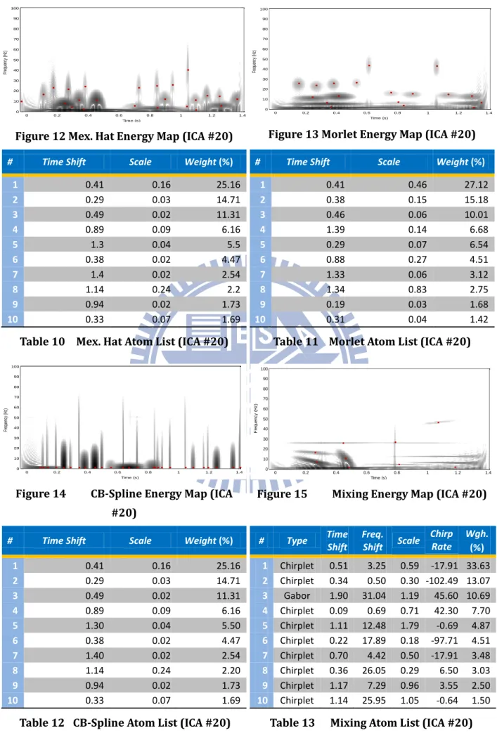
Figure 12 Mex. Hat Energy Map (ICA #20) ... 31

Figure 13 Morlet Energy Map (ICA #20) ... 31

Figure 14 CB-Spline Energy Map (ICA #20) ... 31

Figure 15 Mixing Energy Map (ICA #20) ... 31

Figure 16 Comparison of Convergence Rate of Different Dictionaries over Event Related Potential of Channel #17 ... 32

Figure 17 Gabor Energy Map (Ch. #17) ... 32

Figure 18 Chirplet Energy Map (Ch. #17) ... 32

Figure 19 Mex. Hat Energy Map (Ch. #17) ... 33

Figure 20 Morlet Energy Map (Ch. #17) ... 33

Figure 21 CB-Spline Energy Map (ICA #20) ... 33

Figure 22 Mixing Energy Map (ICA #20) ... 33

Figure 23 Residue and Atom Comparison between Exhaustive MP & Durka’s SMP ... 34

ix

Figure 25 EMP on ICA #20 Chirplet Atom 2 in Table 9 (Typical Failure) ... 35

Figure 26 Uniform Sampling on Y and Z Axis (a) and a More Desirable Distribution of Points Approximating Uniform Sampling on a Sphere (b) ... 38

Figure 27 Energy Distribution of 3 Adjacent Gabor Atoms Generated using Grassmannian Lattice Points ... 41

Figure 28 Relation between Dictionary Mutual Coherence and Redundancy ... 42

Figure 29 Searching for Additional Vectors without Lowering Mutual Coherence ... 44

Figure 30 Dilation/Shrinking Effect of Scaling Factors ... 44

Figure 31 Scatter Plot of the Gabor Parameter Centers ( ) ... 52

Figure 32 Natural Gradient Search over Signal Inner Product Space (ICA #20) Initialization Point = (0.3s, 130rad/s), Grid Redundancy ρ = 0.5 ... 53

Figure 33 Proximity Lattice of Manhattan Distance 2 ... 54

Figure 34 Gabor Energy Map by HyMN-G (ICA #20) ... 56

Figure 35 Convergences of Algorithms (Atom Weights & Residues Energies) ... 57

Figure 36 Large Scale Decomposition of 30 ICA Components (10 Epochs) ... 60

Figure 37 Large Scale Decomposition of 31 Channels (10 Epochs) ... 61

Figure 38 Channel #4, Epoch #155 and Linear Trendline ... 62

Figure 39 Illustration of Noisy Signal Factorization Problem ... 64

Figure 40 K-SVD Decomposition of Channel 17 ERP ... 66

x

List of Tables

Table 1 Mallat’s Matching Pursuit Algorithm ... 7

Table 2 Durka’s Stochastic Matching Pursuit Algorithm ... 8

Table 3 Canonical Memetic Algorithm ... 14

Table 4 Size/Dimension Variables and Their Meanings ... 21

Table 5 Atom A and B with Significant Different Parameters ... 24

Table 6 Atom A and B with Significant Different Parameters ... 26

Table 7 Exhaustive Matching Pursuit Algorithm (Gabor example) ... 29

Table 8 Gabor Atom List (ICA #20) ... 30

Table 9 Chirplet Atom List (ICA #20) ... 30

Table 10 Mex. Hat Atom List (ICA #20) ... 31

Table 11 Morlet Atom List (ICA #20) ... 31

Table 12 CB-Spline Atom List (ICA #20) ... 31

Table 13 Mixing Atom List (ICA #20) ... 31

Table 14 Gabor Atom List (Ch. #17) ... 32

Table 15 Chirplet Atom List (Ch. #17) ... 32

Table 16 Gabor Atom List (Ch. #17) ... 33

Table 17 Chirplet Atom List (Ch. #17) ... 33

Table 18 Gabor Atom List (Ch. #17) ... 33

Table 19 Chirplet Atom List (Ch. #17) ... 33

Table 20 Gabor Atom List Generated by Exhaustive MP (ICA #20) ... 34

Table 21 Gabor Atom List Generated by Durka’s Stochastic MP (ICA #20) ... 34

Table 22 Memetic Pursuit Procedure ... 54

Table 23 Hybrid Memetic Natural Gradient Algorithm ... 55

1

Chapter 1. Introduction

1.1. Motivation

Electroencephalograms (EEGs) have gained its popularity in neurological research and clinical applications due to their mostly non-invasive recording procedures, simple and inexpensive operations and high time resolutions. Originally, the clinical application of EEG analysis is to distinguish epileptic seizures from normal brain activities such as syncope, sub-cortical movement disorders and migraine variants. Advanced signal processing techniques such as independent component analysis (ICA) [1,2] and event related spectral perturbation (ERSP) analysis [3,4] have also become increasingly popular in clinical brain research. In recent years, researchers began to view multichannel EEG recordings as correlated signals with quasi-sparse representations and analyze them with the powerful arsenal of digital signal processing techniques.

However, due to the fact that the recording of EEG for a meaningful and accurate analysis is often necessarily time consuming; the relatively high time resolution and the characteristic of concurrent multichannel recording will produce enormous amounts of data needed to be stored and transported over media. Therefore, interests in searching for sparse and compressible representations of EEG have rose considerably during recent decades.

1.2. Recent Difficulties and Solutions

Unfortunately, determining whether a signal can be optimally approximated and decomposed with a linear expansion over a redundant (over-complete) dictionary of atomic waveforms is an NP-complete problem, furthermore, finding such a solution is an NP-hard one [5]. However, an approximate method that has already been discovered long before is found to be capable enough to tackle this problem. It was the Matching Pursuit algorithm [6]

2

proposed by S. Mallat and Z. Zhang in 1993, which is a simple and economical way to produce a sub-optimal signal expansion by iteratively choosing the atom that best matches the signal structure and remove the atom ingredient from the signal until certain stopping condition is met. This algorithm has already been well studied and improved in the most recent decade, such as the randomized variant – the Stochastic Matching Pursuit (SMP) – pioneered by Piotr J. Durka in 2001.

Despite these efforts, sparse representation remains an impalpable objective. It’s well-known that the sparse decomposition result produced by SMP is possible, however unlikely, to be inconsistent. The dominant atoms in the decomposed sequences for one signal can be significantly different between multiple instances of SMP operations.

1.3. Objectives

The ultimate objective of this research is to identify the dictionary suitable for sparse representation of the EEG ERP signals and components, then design a Memetic Algorithm adopting the belief of Matching Pursuit, which is able to factorize a given EEG signal into a linear combination of only a small number of time-frequency atoms (Gabor functions, for instance) over a redundant dictionary, meanwhile preserving a large portion of signal energy.

1.4. Research Approach

The sparsity of data assumed the ability of representing signals as linear combinations of only a small amount of atoms in a redundant, pre-specified dictionary. This requires the prior knowledge on the signal characteristic and a properly chosen dictionary.

In the aspect of prior knowledge to the signals, researchers performing brain activity analysis based on the equivalent electric dipole modeling [7,8] believed that the stimulus and response events may be well modeled as equivalent dipoles oscillating locally at certain

3

time period and frequency band. So far, on the aspect of proper selection of the dictionaries, Ron Rubinstein et al. indicated that there are two mainstream methods for searching for the proper redundant dictionary [9] currently.

1.4.1. Dictionary Chosen According to Mathematical Model of Signals

The build-up of dictionaries according to mathematical model is mainly functions with closed form mathematical expressions such as Gabor functions and wavelet atoms, which can be easily parameterized.

Further, about the searching method for the representation in the various types of standard dictionaries, while Durka’s Stochastic MP algorithm focuses mainly on bias elimination and generates only sequences of atoms with integral multiplications of sampling steps over the time and frequency domain, a new method employing advanced optimization algorithms is proposed to improve the accuracy and efficiency of parameter searching in each MP iterative step by regarding the parameters as continuous variables and providing an even sparser parameterized representation.

1.4.2. Dictionary Evolved Based on Training Data

This type of dictionaries emerges, in Ron’s words [9], from a given set of realizations of the data. This set serves as the examples of the signals to be modeled; with a given initial dictionary, the training algorithm will evolve the dictionary atoms iteratively to make the resulted dictionary performs better on the training set. In such case, an initialization method with minimal mutual coherence based on the Grassmannian frame for the dictionary is proposed to enhance the learning procedures.

1.5. Contributions

4

find a decomposition sequence in the scalable Gabor dictionary, which improves the Matching Pursuit by extending the search space into continuous real number domain and with one more degree of freedom with variable scaling factors. With the behaviors of the parameters of the Gabor standard dictionary are well understood, the signal can therefore be decomposed into merely a small number of parameter sets with minimal energy losses.

Another contribution is the successful application of the K-SVD on the EEG signal integrated with the concept of Grassmannian frames; the resulted dictionary contains several fingerprints of the event related potential of the EEG signal, which might be used further to identify different stimuli with the help of classification methods.

1.6. Thesis Outline

Along the roadmap, in Chapter 2, the fundamental tools and prior knowledge will be introduced. Each succeeding chapters will focus on each milestone of major discoveries.

In Chapter 3, the identification of Gabor atoms as the most suitable type of waveform and an intuitive, however stable and consistent method based on Matching Pursuit to find the representation are described here, including some first-stage experiment results.

In Chapter 4, a better optimization method based on Natural Gradient and a sub-optimal uniform sampling method over Gabor parameter space using the Grassmannian concept will be introduced. The experiment results will be compared with their counterpart mentioned in Chapter 3. The Chapter 3 and Chapter 4 will cover the approach of realizing sparse representation via overcomplete standard waveform dictionaries.

Chapter 6 describes the improvements on the K-SVD algorithm via a new dictionary

initialization method using the Grassmannian frame; the experiment result will be compared to the default initialization method using the normalized random Gaussian noise.

5

Chapter 2. Backgrounds

In recent years, a new signal processing paradigm called Compressive Sensing (CS) [10,11] promises to reduce the representation data size of a sparse signal up to two orders of magnitude while capturing their essential characteristics. The key to efficient compressive sensing and sparse signal analysis lies with successful identification of suitable signal dictionaries for the sparse representation of those signals.

A preliminary study by S. Aviyente in 2007 [12] suggested that the compressive sensing framework might be applicative for EEG signals. In 2009, Abdulghani et al [13] demonstrated the apparent sparsity of EEG signals with respect to several standard dictionaries including the Gabor atoms, Mexican Hat and Spline-based wavelets. However, the proper temporal-frequency and spatial-temporal dictionaries are yet to be discovered.

2.1. Gabor Atoms and Dictionary

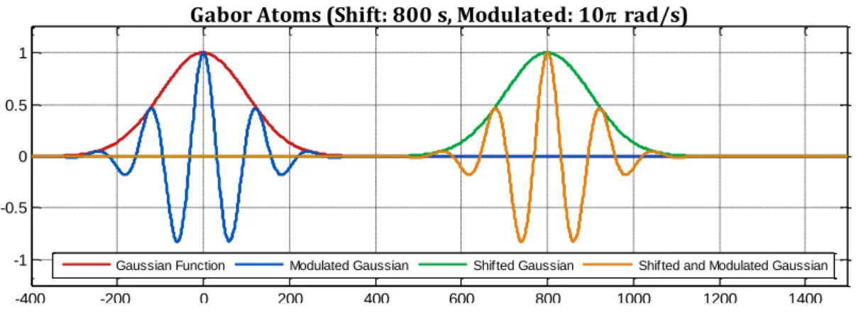
Real Gabor atoms, which are simply shifted and frequency modulated Gaussian functions, which can be expressed as follow:

𝑔𝛾 𝐾(𝛾)𝑒−𝜋(𝑡−𝑡0)2∕𝑠2cos(𝜔0(𝑡 − 𝑡0) + 𝜙) (1

The set 𝛾 *𝑡0 𝜔0 𝑠 𝜙+ in the parameter space Γ is the parameter set of a Gabor

function, which contains the time center 𝑡0, the frequency center 𝜔0, temporal scaling

factor 𝑠 and the sinusoidal phase 𝜙 of the atom. The normalization factor 𝐾(𝛾) is the function ensuring the atom contains unit norm energy.

Figure 1 gives an example of Gabor atom (not energy normalized) waveforms in the time domain as shifted and modulated Gaussian functions.

6

Figure 1 Gabor Atoms as Shifted and Modulated Gaussian Functions

The Gaussian envelope of a Gabor atoms leads to the optimal time-frequency localization for the Heisenberg’s uncertainty principle in terms of energy concentration (the equality holds if 𝑔 is a Gaussian function):

𝜍𝑡2𝜍𝜔2 (∫ 𝑡2|𝑔(𝑡)|2𝑑𝑡 ∞ −∞ ) (∫ 𝜔∞ 2_{|𝑔̂(𝜔)|}2_𝑑𝜔 −∞ ) ≥ ‖𝑔‖ 4 16𝜋2 (2

This property makes the Gabor atom suitable for performing local time-frequency brain activity observations and analyses; an explicit construction method for an overcomplete Grassmannian Gabor frame will be introduced later.

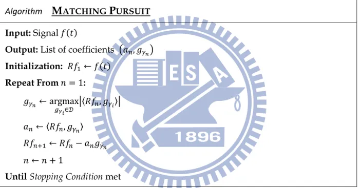
2.2. Matching Pursuit

2.2.1. S. Mallat’s Matching Pursuit (MP)

Matching pursuit (MP) algorithm can provides a sub-optimal solution to the problem of acquiring an adaptive approximation of a signal in a redundant set of waveforms (dictionary). The pursuit starts with a given dictionary with sufficiently abundant of unit energy

atoms 𝒟 ≡ {𝑔𝛾𝑛 ∶ ‖𝑔𝛾𝑛‖ 1}_𝑛=1

𝑁

of size 𝑁 and a signal 𝑓(𝑡) to be analyzed; the main

goal is to find a linear combination of atoms approximating the signal 𝑓(𝑡):

-400 -200 0 200 400 600 800 1000 1200 1400 -1 -0.5 0 0.5 1

Gabor Atoms (Shift: 800 s, Modulated: 10 rad/s)

7

𝑓(𝑡) ≈ ∑ 𝑎_𝑛𝑔_𝛾𝑛(𝑡)

𝑛

(3

In each iterative step, the algorithm chooses the atom having the largest inner product with the signal from 𝒟. The signal is then subtracted by the atom waveform weighted by the inner product value. The procedure is repeated on the subsequent residual 𝑅𝑓𝑛(𝑡) after the

subtractions until certain stopping condition is met, such as an acceptable energy extraction threshold or the number of iterations limited.

Algorithm

M

P

Input: Signal 𝑓(𝑡)

Output: List of coefficients (𝑎𝑛 𝑔𝛾𝑛)

Initialization: 𝑅𝑓1 ← 𝑓(𝑡) Repeat From 𝑛 1: 𝑔_𝛾𝑛 ← argmax 𝑔_𝛾𝑖∈𝒟 |〈𝑅𝑓𝑛 𝑔𝛾𝑖〉| 𝑎𝑛 ← 〈𝑅𝑓𝑛 𝑔𝛾𝑛〉 𝑅𝑓_𝑛+1 ← 𝑅𝑓_𝑛− 𝑎_𝑛𝑔_𝛾𝑛 𝑛 ← 𝑛 + 1

Until Stopping Condition met

Table 1 Mallat’s Matching Pursuit Algorithm

The orthogonality of the residue 𝑅𝑓𝑛+1 and the best matched atom 𝑔𝛾𝑛 selected in

the 𝑛Th iteration implies the signal energy conservation property:

‖𝑓‖2 _{∑|〈𝑅𝑓} 𝑛 𝑔𝛾𝑛〉| 2 𝑁 𝑛=1 + ‖𝑅_𝑁+1𝑓‖2 _∑|𝑎 𝑛|2 𝑁 𝑛=1 + ‖𝑅_𝑁+1𝑓‖2 ₍₄

This implies that if the algorithm successfully extracts the atom with the maximum correlation with the signal in each iteration step, the residue will consequently be minimized in terms of signal energy.

8

2.2.2. Stochastic Matching Pursuit

In 2001, Piotr J. Durka has proposed the Stochastic Matching Pursuit algorithm (SMP) [14], which is a Monte Carlo approach aiming to find a statically unbiased linear expansion for quasi-sparse signals.

Algorithm

S

M

P

Input: Signal 𝑓(𝑡)

Output: List of coefficients (𝑎𝑛 𝑔𝛾𝑛)

𝑔𝛾1 ← argmax

𝑔_𝛾1∈𝒟 |〈𝑓 𝑔𝛾1〉|

Take arbitrary percentages of atoms with large correlation with 𝑓(𝑡) to form 𝒟𝛼

𝑎₁ ← 〈𝑓 𝑔_𝛾1〉 𝑅𝑓2 ← 𝑓 − 𝑎1𝑔𝛾1 Repeat From 𝑛 2:

Generate 𝒟𝑒 densely and exhaustively in the parameter center of atoms in 𝒟𝛼

𝑔_𝛾𝑛 ← argmax 𝑔_𝛾𝑖∈𝒟𝑒 |〈𝑅𝑓_𝑛 𝑔_𝛾𝑖〉| 𝑎𝑛 ← 〈𝑅𝑓𝑛 𝑔𝛾𝑛〉 𝑅𝑓_𝑛+1 ← 𝑅𝑓_𝑛− 𝑎_𝑛𝑔_𝛾𝑛 𝑛 ← 𝑛 + 1

Until Stopping Condition met

Table 2 Durka’s Stochastic Matching Pursuit Algorithm

First, a stochastic dictionary 𝒟 is generated according to the required signal length 𝑁 and chosen time-frequency resolutions in time, frequency and scale (Δ𝑡 Δ𝜔 and Δ𝑠). The parameter space is thereby divided into total 𝜋𝑁2⁄Δ𝑡Δ𝜔Δ𝑠 cuboids of size Δ𝑡 × Δ𝜔 × Δ𝑠. In each cuboid, a Gabor atom is chosen by drawing its parameters from uniform distributions within the given ranges of continuous parameters.

In the first iteration, a percentage of prominent atoms with large correlations with the input signal are chosen to form an adaptive dictionary 𝒟𝛼. Afterwards in each matching

9

procedure, parameters of the atoms chosen from 𝒟𝛼 are further optimized by a dense and

exhaustive search in the designated vicinity.

In [14], Durka stated that, instead of being driven by a quest to improve the speed or compression ratio, the goal of the stochastic method is attaining possible exact parameterization of certain signal structures freeing from bias and with a constant time-frequency resolution.

2.3. Localized Optimization Methods

The localized optimization methods are employed on the parameter sets of the time-frequency atoms to maximize the correlation between the atom waveform and the input signal or residuals. Two of which that have been employed during the research period are listed below.

2.3.1. Covariance Matrix Adaptation Evolution Strategy

The Covariance Matrix Adaptation Evolution Strategy (CMA-ES) is a stochastic numerical optimization method. As the tradition of the evolution strategies, each new generation of candidates are sampled according to a multivariate Gaussian distribution based on the pairwise dependencies between the variables in the parameter sets – the dependencies in the distribution are described by a covariance matrix. The covariance matrix adaptation (CMA) is a method to update the covariance matrix of this distribution.

2.3.2. Natural Gradient

Generic optimization algorithm (black-box optimization) are designed for problem with unknown and sophisticate objective functions; one of the simplest and the most celebrious one is gradient based optimization, based on the fact that a minimum or a maximum of a function takes place at the point having zero partial derivatives in all dimensions, forming the

10

core concept of gradient descent/ascent method [15,16]. One of the most significant advantages of gradient descent over the other alternatives is the simplicity and efficiency; however, the most notable drawback is the vulnerability towards local minimum, especially when the objective function is mountainous, asperous or spiky.

In 1998, S. Amari et al introduced the natural Riemannian gradient or simply, natural gradient [17,18] in the field of optimization. Taking the curved space into consideration and changes the concept of distance in ordinary Euclidean space.

In 2008, Daan Wierstra and Tom Shaul presented the Natural Evolution Strategy (NES) [19,20], utilizing the canonical process of the gradient descent but replacing the standard gradient by empirical Natural Gradient derived using population based method to estimate Fisher information matrix and gradient of the objective function.

The next year in 2009, with Yi Sun's help in advance, the Natural Evolution Strategy benefited from a new computational method to attain actual Fisher information matrix instead of performing population based estimation on the objective function in the parameterized searching space. This improved version of the algorithm is called Efficient Natural Gradient Strategies [21].

In this research, the natural gradient based algorithms are employed as local optimization method to seek for the best atom parameter to decompose the signal.

2.4. Grassmannian Frame

This section includes the mathematical property of a frame, since frames with low mutual coherence are favored in the field of Compressive Sensing; the Grassmannian concept is employed to suppress the increment of mutual coherence when raising the redundancy of a dictionary.

11

2.4.1. Frame and Mutual Coherence

An 𝑁- element finite frame 𝑋_𝑑𝑁 *𝑥1 𝑥2 … 𝑥𝑁+ ⊆ ℝ𝑑 is a family of vectors that

characterizes any signal from its inner product *〈𝑓 𝑥𝑘〉+ and completely spans the

𝑑-dimensional Euclidean space, which necessitates 𝑁 ≥ 𝑑 and should hold the frame condition: There exists two constants 𝐴 and 𝐵 𝐴 ≤ 𝐵 for any function 𝑓 ∈ ℝ𝑑 such that 𝐴‖𝑓‖ ≤ ∑ |〈𝑓 𝑥𝑘 𝑘〉|2 ≤ 𝐵‖𝑓‖.

Of particular concern is the correlation value between the underlying atoms within frame, which is known as the mutual coherence of a frame. The definition is:

𝜇(𝑋𝑑𝑁) max_{𝑘 𝑙∈Γ 𝑘≠𝑙} |𝑥𝑘𝑇𝑥𝑙| 𝑥_𝑘𝑇_𝑥 𝑘𝑥𝑙𝑇𝑥𝑙 ≥ √ 𝑁 − 𝑑 𝑑(𝑁 − 1) (5

The maximum correlations are ideally zero for all orthonormal frames; for overcomplete dictionaries, those with small mutual coherence value are preferred in the case of sparse representation. The effect will be discussed later in 3.6.

2.4.2. Definition of Grassmannian Frames

A unit-energy (unit 𝐋2 norm) finite frame 𝑈𝑑𝑁 *𝑢1 𝑢2 … 𝑢𝑁+ ⊆ ℝ𝑑, where |𝑢𝑛| 1

∀𝑛 1 to 𝑁, is an (𝑁 𝑑)-Grassmannian frame [22] if satisfying the minimal mutual coherence criterion:

𝜇(𝑈_𝑑𝑁_{) inf{𝑋}

𝑑𝑁} (6

That is, the 𝑁 −element Grassmannian frames are frames minimizing the mutual coherence in ℝ𝑑. In [22], T. Strohmer et al provided a method of constructing optimal Grassmannian frame with Gabor atoms by positioning the time and frequency center of the atoms on a triangular lattice over continuous time-frequency plane.

12

2.4.3. Grassmannian Gabor Frame

Recent attempts to represent a vector/function/operator in terms of a redundant spanning set of normalized elements gives rise to the concept of frames, which can be regarded as the generalization of orthonormal bases. The level of its over-completeness is measured by its redundancy 𝜌. Recently, about the acquisition of Grassmannian Gabor frame, T. Strohmer introduced two unitary operators of translation 𝑇𝑥 and modulation 𝑀𝜔 in [22]:

, 𝑇𝑡0𝑓(𝑡) 𝑓(𝑡 − 𝑡0)

𝑀_𝜔0(𝑡) 𝑓(𝑡)𝑒𝑗𝜔0𝑡 (7

A two dimensional lattice Λ is a discrete subgroup of time-frequency parameter space with compact quotient determined by a generator matrix 𝐿 via Λ 𝐿℞2. The volume of the lattice Λ is vol(Λ) det(Λ). For the Gaussian window function 𝑔 ∈ 𝐋2(ℝ) and a lattice Λ in the time frequency plane ℝ2, the corresponding Gabor system can be defined as:

𝒢(𝑔 Λ) {𝑀𝜔0𝑇𝑡0𝑔 where (𝑡0 𝜔0) ∈ Λ} (8 The completeness of the system is therefore determined by the redundancy 𝜌 1 vol(Λ)⁄ . A necessary condition for a Gabor system 𝒢(𝑔 Λ) to be a frame is 𝜌 ≥ 1.

Since a Gaussian function in time domain remains Gaussian in frequency, also, both shift and rotational invariant with respect to every time frequency center (𝑡0 𝜔0). The time

frequency energy spread is an ellipse in the time frequency plane, the redundancy of the Gabor system can be viewed as the overlapping in time-frequency energy distribution.

Applying the classical sphere packing theory [23], the optimal lattice for a two dimensional space is the solution for argmaxΛ*(volume of a sphere) × 𝜌+ , and the

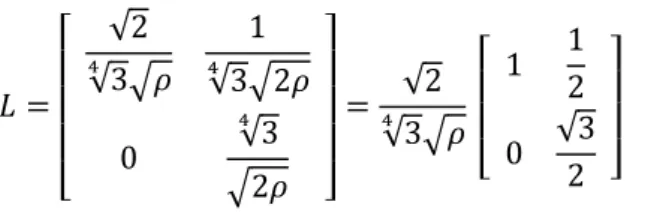
13 𝐿 [ √2 √3 4 √𝜌 1 √3 4 √2𝜌 0 √3 4 √2𝜌 ] √2 √3 4 √𝜌 [ 1 1 2 0 √3 2 ] (9

Such result is also applied on OFDM design for time-frequency dispersive channel, the Fig. 4 (b) in [24] illustrate the resulted Gabor system energy concentration of the packing:

Figure 2 Supports of Energy Spreading of a Constant-Scale Gabor System Generated with a Hexagonal Lattice, Fig. 4 (b) of [24]

And the dilation effect of the scaling factor would make the form become:

𝐿_𝑠 √ 2 √3𝜌 [ 𝑠 𝑠 2 0 √3 2𝑠 ] (10

The overcomplete Grassmannian Gabor frame will be applied on both the advanced search of the optimal standard waveform representation and the dictionary training approach as well; from which the Matching Pursuit based algorithm selects the most prominent atom then performs further optimization in the first approach, and serves as the initial dictionary with configurable redundancy in the second.

14

2.5. Memetic Algorithms

The theory of “Universal Darwinism” was coined by Richard Dawkins in 1983 [25] to provide a unifying framework governing the evolution of any complex system. In particular, “Universal Darwinism” suggests that evolution is not exclusive to biological systems. The term “meme” was also introduced and defined by Dawkins in 1976 as “the basic unit of cultural transmission, or imitation”, and in the English Oxford Dictionary as “an element of culture that may be considered to be passed on by non-genetic means”.

Now, Memetic Algorithm (MA) [26] is one of the recent blooming areas of research in evolutionary computation, which is now widely used as a synergy of population-based approach with separate individual local improvement procedures. And finally, use evolutionary strategy such as Darwinian or Lamarckian filtering to select the proper chromosomes to reproduce the next generation.

The following code section shows a typical process of a canonical Memetic Algorithm:

Algorithm

C

M

A

Initialize: Given starting point 𝑝;

While Stopping conditions Not satisfied Do

Evolve a new population Π using stochastic search operators. Evaluate all individuals in the population.

Select the subset of individuals Ω𝑖𝑙 that should take the learning procedure.

For Each individual In Ω𝑖𝑙 Do

Perform learning with meme with probability of 𝑝𝑖𝑙 Proceed with Lamarckian or Baldwinian learning.

End For End While

Table 3 Canonical Memetic Algorithm

15

dictionary and the natural gradient based search algorithm to assemble the ultimate optimization method for the search of the Gabor parameter whose corresponding waveform fit the given signal the most.

16

Chapter 3. CMA-ES Based Local Search

Based on the fundamental belief of Matching Pursuit, the goal of searching for the parameters of atom having the highest correlation value with the signal is quite obvious. In the first move, the quasi sparse characteristic of the EEG signals is justified by observing the distribution of Gabor atom centers from the result of time frequency analyses.

3.1. Identifying the Quasi Sparse Property of EEG Signals,

17

Each time-frequency-scale central point is weighted by the squared correlation value between the atom waveform and the signal according to the energy conservation property in Equation (4. To emphasis the concentration, a spherical kernel density function is used, the mathematical formula of the kernel is:

{ 𝑘 ⋅ (1 − 𝑡2)2 if 𝑡 < 1

0 if 𝑡 ≥ 1 where 𝑡 is the distance measure (11

The concentration of time-frequency centers of Gabor dictionary atoms generated by decomposing the EEG signal with Durka’s stochastic matching pursuit indicates the possibility of representing the signal with only few time-frequency localized atoms.

3.2. Sparse Representation over Standard Dictionaries

This section contains the description of four types of dictionaries – Gabor Chirp (Chirplet), Morlet wavelet, real Mexican Hat Wavelet and Cubic Cardinal B-Spline – used to obtain the sparse representation of the ERP and ICA signals.

3.2.1. Linear Gabor Chirp (Linear Chirplet) Dictionary

A linear Gabor chirp, or a chirplet by Steve Mann [27], is a piece of a chirp derived from windowing a chirp function where the window provides the time localization property similar to their Gabor siblings.

Most of the chirplet parameters are the same as those used in the Gabor atom, the additional parameter, the chirp rate, is introduced to represent the change of the oscillating frequency of the waveform over time.

Given the parameter set *𝑡0 𝜔0 𝑠 𝑐 𝜙+ as time center, frequency center, scale, chirp

rate and phase, the mathematical formula of a chirplet atom is:

𝑔_{𝑡0 𝜔0 𝑠 𝑐 𝜙}(𝑡) 𝐾 ∙ exp (−𝜋 (𝑡 − 𝑡0

𝑠 )

2

) ⋅ cos (𝑐(𝑡 − 𝑡0)2

18

The normalizer 𝐾 is a parameter set dependent function employed here and in the following sections to generate unit-norm atoms.

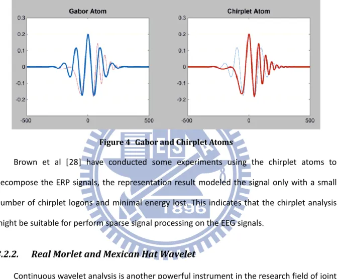
The following figure gives an example for a Gabor atom and a chirplet atom with the same time-frequency center, scale and phase.

Figure 4 Gabor and Chirplet Atoms

Brown et al [28] have conducted some experiments using the chirplet atoms to decompose the ERP signals, the representation result modeled the signal only with a small number of chirplet logons and minimal energy lost. This indicates that the chirplet analysis might be suitable for perform sparse signal processing on the EEG signals.

3.2.2. Real Morlet and Mexican Hat Wavelet

Continuous wavelet analysis is another powerful instrument in the research field of joint time-frequency analysis [29,30]. As the ordinary constant-scale Gabor analysis (or short-time Fourier analysis) emphasized the localized time and frequency activities using time shifts and frequency modulations; the wavelet provides an alternative for frequency modulations by changing the scaling factors. According to the Heisenberg’s uncertainty principle, a lower scaling factor will narrow the active period in time but expands the observable frequency band, and a larger one will do the opposite.

19

windowed sinusoid and actually embedded in the subspace of the Gabor atoms. Given the sampling rate 𝑓 and the parameter set *𝑡0 𝑠+ the parameterized Morlet atom can be

represented as: 𝜓𝑡0 𝑠(𝑡) 𝐾 ⋅ exp (− 1 2( 𝑡 − 𝑡₀ 𝑠 ) 2 ) ⋅ cos (5 ⋅ 𝑓 ⋅ (𝑡 − 𝑡0 𝑠 ) 2 ) (13

The Mexican Hat wavelet is proportional to the second order derivative of the Gaussian function. With the parameter set *𝑡0 𝑠+, the shifted and scaled Mexican Hat wavelet atom

can be formulated as:

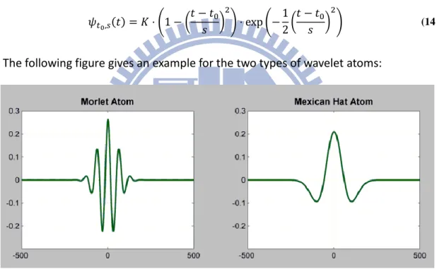
𝜓𝑡0 𝑠(𝑡) 𝐾 ⋅ (1 − ( 𝑡 − 𝑡₀ 𝑠 ) 2 ) ⋅ exp (−1 2( 𝑡 − 𝑡₀ 𝑠 ) 2 ) (14

The following figure gives an example for the two types of wavelet atoms:

Figure 5 Morlet and Mexican Hat Atoms

Both the Morlet and Mexican Hat wavelet families are both widely used in biomedical signal analysis [31,32] and other areas like image compression.

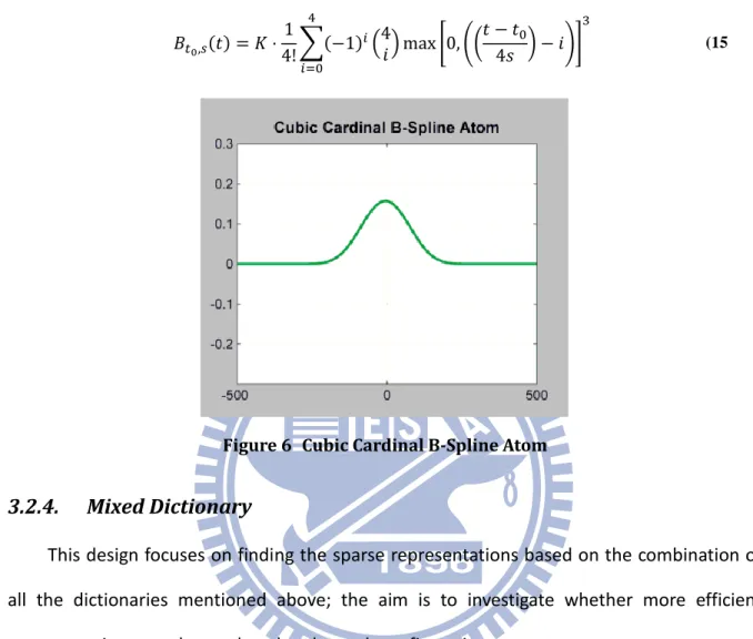
3.2.3. Cubic Cardinal B-Spline

The cubic cardinal B-spline functions are continuous piecewise-polynomial compact waveforms introduced recently [33,34] for sparse representations and biomedical signal processing; these waveforms are frequently employed to absorb pulse-shaped features of

20

the signals. Given the parameter set of time shift and scaling factor *𝑡0 𝑠+, the cubic cardinal

B-spline atom has the following mathematical form as in Equation (15 and shape in Figure 6:

𝐵_{𝑡0 𝑠}(𝑡) 𝐾 ⋅ 1 4!∑(−1)𝑖.4𝑖/ max *0 (( 𝑡 − 𝑡₀ 4𝑠 ) − 𝑖)+ 3 4 𝑖=0 (15

Figure 6 Cubic Cardinal B-Spline Atom

3.2.4. Mixed Dictionary

This design focuses on finding the sparse representations based on the combination of all the dictionaries mentioned above; the aim is to investigate whether more efficient representations may be produced under such configuration.

3.3. Signal Decomposition

3.3.1. Decomposition Problems

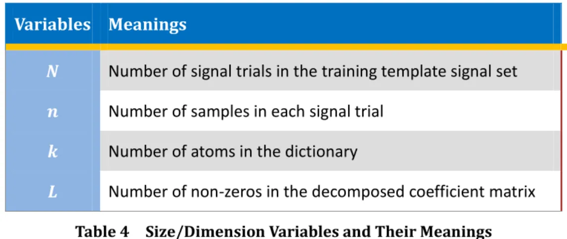
21

Variables Meanings

𝑵 Number of signal trials in the training template signal set

𝒏 Number of samples in each signal trial

𝒌 Number of atoms in the dictionary

𝑳 Number of non-zeros in the decomposed coefficient matrix

Table 4 Size/Dimension Variables and Their Meanings Their relation should be 𝐿 ≪ 𝑛 < 𝑘 ≪ 𝑁.

The sparse signal decomposition (factorization) problem is formally stated here: Let 𝑘 > 𝑛 𝑏 ∈ ℝ 𝐴 ∈ ℝ𝑛×𝑘 _{and Rank(𝐴) 𝑛, the noiseless single-trial signal decomposition}

problem 𝑃0 is defined as:

𝑃0≡ min_𝑥 ‖𝑥‖0 subject to 𝐴𝑥 𝑏 (16

The solution for the problem 𝑃0 is definitely the sparse most representation. However,

the case of the realistic world is not always in such an ideal situation; with the presence of noises, the bounded error version problem 𝑃𝑜 𝜖 with the error measured in terms of the 𝐋2

norm is therefore defined for practice. The 𝑃0 𝜖 problem is suitable for modeling single-trial

quasi-sparse standard waveform decomposition and recovery, which is presented in mathematical equation (17 and illustrated as Figure 7:

𝑃_{0 𝜖} ≡ min

𝑥 ‖𝑥‖0 subject to ‖𝐴𝑥 − 𝑏‖2< 𝜖 (17

Figure 7 Illustration of Noisy Sparse Single-Trial Signal Decomposition Problem

A

b' b

|| b – b' ||₂<ϵ

22

3.3.2. Decomposition Algorithm

For the standard waveform dictionaries, the proposed method is basically based on the iterative procedures of Matching Pursuit.

An improved iteration procedure can be separated into 3 stages:

1. Finding candidate atoms over loosely sampled parameter set

The candidates found in this stage are passed into the next stage as initial configuration of the optimization algorithm.

2. Optimizing the candidates using CMA-ES

The CMA-ES algorithm will search the vicinity of the initial point acquired from the previous stage and iteratively converged to a certain parameter set. The most prominent set maximizing the absolute inner product value of the derived atom will be recognized as the best matched.

3. Removing the best matched waveform from the signal space

This step is the same as the original Matching Pursuit.

To identify in which type of dictionaries can the signal be well and sparsely represented, the Matching Pursuit algorithm is applied on several types of standard dictionary including the generalized Gabor dictionary (consists of Fourier atoms, impulse functions and ordinary Gabor functions), Mexican Hat wavelet, Morlet wavelet and Cubic Cardinal B-Spline dictionaries for the comparison of the performance for each type of dictionary listed above.

23

3.4. Matching Pursuit Based on CMA-ES

Covariance matrix adaptation evolution strategy (CMA-ES) [35,36] is a stochastic numerical algorithm for solving non-linear non-convex optimization problems with search spaces of three to a hundred dimensions.

In essence, CMA-ES performs a principal components analysis in each mutation step so as to provide maximum likelihood estimation for subsequent parameter adaptation. Beside of computing the covariance matrix of its multivariate normal distribution of mutations, it also records the evolution paths of the mean of mutation distribution. The information is used to control the step size of mutations and determine the favorable directions for covariance adaptation. As a result, the algorithm is capable of handling problems with multimodal, discontinuous, even noisy fitness functions.

CMA-ES is a highly reliable and competitive algorithm for most local optimization and many global optimization problems. It is the de-factual benchmark for adaptive optimization.

3.5. Discovery of Inconsistency

Inconsistency described here means the decomposition sequences of the Gabor atom parameter sets may have significant differences in atom orders and values.

Given the same signal, the dominant atoms of one representation can be significantly different from those appear in another representation produced by a different run of the algorithm. Two causes of inconsistency have been identified:

1. The presence of redundant atoms in a dictionary

For example, multiple atoms in a Gabor dictionary can produce similar or identical waveform; if the oscillating frequency of the sinusoid is too low, the behavior of the atom is just similar to a single envelope without oscillating. For

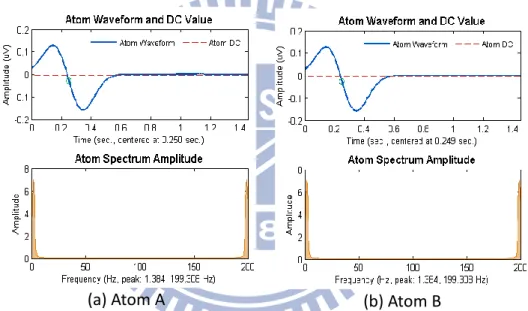
24

example, the two following unit-energy atoms 𝐴 and 𝐵 have almost identical waveform (both contain 290 sampling points at sampling rate of 200 Hz):

Atom Length ( ) Normalizer Shift ( ) Freq. (Hz) Scale( ) Phase (𝝅)

𝑨 1.45 36.486077 0.2491 0.0101 0.2533 0

𝑩 1.45 0.538988 0.25 0.6897 0.26 0.5172

Table 5 Atom A and B with Significant Different Parameters

The mean square error is ‖𝐴 − 𝐵‖2⁄290 2 7338 × 10−7, and the following Figure 8 shows the waveform and frequency spectrum of the two atoms.

(a) Atom A (b) Atom B

Figure 8 Example of Two Almost Identical Atoms with Different Parameters

2. The existence of degenerative cases in a sparse representation

For example, as a Gabor atom increases the standard deviation of its Gaussian envelope, it becomes more difficult to locate the time center of this atom.

In “Consistent Sparse Representations of EEG ERP and ICA Components Based on Chirplet and Wavelet Dictionaries” * 37 ], several constraints on value ranges of the parameters are proposed to ensure the consistency during the decomposition.

25

3.6. Consistency Conditions

For signal decomposition algorithms, there are several indexes for performance measurements – accuracy, efficiency and consistency [37]:

The accuracy of the decomposition is measured in the strength of the correlation between the found atom and the signal; the efficiency is ranked in terms of the number of atoms used to absorb a certain percentage of energy; the consistency is judged based on following two terms:

1. The organization of the decomposed atoms

The ensemble of dominant atoms should form distinct clusters in their parameter spaces; these clusters of atoms accumulated through repeated random searches may be used to classify different ERP types.

2. The reflections of ERP signal atoms in ICA components

The clusters of dominant atoms of ERP signals and their ICA components should manifest significant overlap with one another ― these overlap atom clusters confirm the agreement between the sparse representations of the two EEG signal forms.

To ensure consistency, the decomposition should first have uniqueness (for exact reconstruction of noiseless signals), or stability (for signals with noise) through the sparsity of signals, which will be covered in 3.6.1; and the rule enforcing parameter consistency will be discussed in 3.6.2.

3.6.1. Mathematical Uniqueness and Stability

In 2003, Donoho and Elad [38,39] identified the harsh conditions for the existence of a unique and stable representation in an over-complete dictionary. Elad et al. [40] then

26

proposed a method to find a unique dictionary that can produce stable representations for a given set of signals and devised the K-Singular Value Decomposition (K-SVD) algorithm [41] to design the dictionary consisting of non-parametric atoms with tailored waveforms only if the existence conditions of stable representations were satisfied at the first place; the part of the KSVD algorithm will be stated later in Chapter 6, here, the primary focus is the uniqueness and consistency condition on single-trial signal decomposition.

In [40] it describes that if the sought solution 𝑥 for 𝑃0 satisfies the sparsity condition,

‖𝑥‖0≤

1 2(1 +

1

𝜇(𝐴)) (18

the pursuit algorithms will recover the original signal exactly. This suggest that for representation less than 𝒪(√𝑛) non-zero terms (see equation (5 ), Matching Pursuit algorithm can successfully reconstruct the signal.

3.6.2. Parameter Consistency

The Gabor parameters of different atoms span the search space of the CMA-ES. In order to exclude the redundant and degenerative cases in CMA-ES mutations, the following pruning rules of the search space are devised to prevent such undesired occasions:

Rule Parameters Pruning Rules (Tolerance: ± %)

1

2

3

4

5

where 𝜔𝜓 central frequency of the wavelet mother function.

27

In rule 1 and 2, pruning of (𝑡0 𝜔0) is meant to ensure that the chosen atoms always

fall within the time and frequency spans of the target signal. Applying these rules will eliminate most of the redundant atoms.

In rule 3, replacing the Gabor atoms with 𝑠 > 100 by Fourier atoms of the same frequency is meant to remove degenerated Gabor waveforms. The replacement will only be carried out if the inner product 〈𝑟𝑚(𝑡) 𝑔𝛾𝑚(𝑡)〉 of the Fourier atoms is large than those of

the Gabor atoms.

In rule 4 and 5, discarding chirplet and wavelet atoms with large scale is meant to eliminate degenerated waveforms, whose spectra spread across the entire frequency band.

3.7. Experiments

Here, the type of dictionary that is the best choice for decomposing the EEG signal will be identified, and a simple method will be introduced to achieve consistent results.

3.7.1. EEG Signal Recording and Pre-processing

A 64-channel EEG signal recording session was conducted within an EM-insulated chamber in NCTU Brain Research Centre (BRC) in July 2009. During the recording session, the test subject was asked to listen to a randomized sequence of rising or falling tones and was instructed to press a button immediately after hearing the rising tone but do nothing otherwise. The entire session lasted 40 minutes and produced total 1600 auditory-motor ERP epochs.

The signals from all 62 scalp channels were sampled into single-precision (16 bit) data at 1 KHz sampling rate and passed through ideal 1 Hz – 75 Hz FFT filters. They were then down sampled to 200 samples per second and fed through the artefact removal procedures. Only 266 epochs of the no bottom pressing event and 108 epochs of the bottom pressing ones remained after the procedure. Each epoch contain 290 samples that cover a period from

28

40ms before to 1405ms after each Event On-Set (EOS) moment. Independent component analysis was then applied to all the epochs to produce their corresponding ICA components. Average ERP signals of the two events were generated by removing the DC components of individual epochs and then averaging their signal samples. Similar process was used to produce the average ICA components.

3.7.2. Experiment Configurations

The experiment goal in this early phase of the research period is to identify correctness and guarantee stability of the decomposition result, and select the most promising dictionary that can appropriately decompose the EEG signal with the smallest amount of atoms required for later use.

Let the signal elapses for 𝒯 and has the bandwidth of ℬ, the resolution in time, angular frequency and scale is respectively Δ𝑡 Δ𝜔 and Δ𝑠 (scaling factors 𝑠 and Δ𝑠 have the same unit as time shifts 𝑡0 and Δ𝑡, both are time units). The following algorithm is implemented to

decompose the signal in a trivial way (the restriction of scaling factor 𝒮min and 𝒮max is

29

Algorithm

E

M

P

(EMP)

(

G

)

Input: Signal 𝑓(𝑡)

Output: A list of coefficients and waveform parameters (𝑎𝑛 𝛾𝑛)

Initialization: 𝑅𝑓1 ← 𝑓(𝑡);

While 𝑛 1 to Iteration Limit and Stopping Condition not met

𝑎_max ← −∞; 𝛾_max ← 𝑁𝑢𝑙𝑙

For 𝑡0 0 to 𝒯 step Δ𝑡

For 𝜔0 0 to ℬ step Δ𝜔

For 𝑠 𝒮min to 𝒮max step Δ𝑠

𝛾 ← ,𝑡0 𝜔0 𝑠0-; 𝑎 ← 〈𝑅𝑓𝑛 𝑔𝛾〉

If |𝑎| > 𝑎_max then

(𝑎_max 𝛾_max) ← (𝑎 𝛾) # the most correlated atom

End If End For End For End For

𝛾_𝑚𝑎𝑥′ _{← 𝑪𝑴𝑨𝑬𝑺(𝛾}

max) # local optimization procedure with pruning rules

𝑎𝑚𝑎𝑥′ ← 〈𝑅𝑓𝑛 𝑔𝛾𝑚𝑎𝑥′ 〉 # use the updated correlation value

(𝑎n 𝛾n) ← (𝑎max′ 𝛾max′ )

𝑅𝑓𝑛+1 ← 𝑅𝑓𝑛− 𝑎𝑛𝑔𝛾𝑛 End While

Table 7 Exhaustive Matching Pursuit Algorithm (Gabor example)

The objective function is simple, given the parameter set 𝛾; the object function returns the value |〈𝑅𝑓𝑛 𝑔𝛾〉|. For the wavelets, simply remove the frequency scanning loop of 𝜔0.

3.7.3. Experiment Results

This experiment was suggested to use the event related potential of ICA component 20 and channel 17 as our input. (Signal elapse 𝒯 1 45, Bandwidth ℬ 75Hz).

30

Figure 9 Comparison of Convergence Rate of Different Dictionaries over ICA Component #20

Figure 10 Gabor Energy Map (ICA #20) Figure 11 Chirplet Energy Map (ICA #20)

# Time Shift Freq. Shift Scale Phase ( ) Wgh. (%) 1 0.52 1.70 0.71 1.37 30.04 2 0.32 6.24 0.15 1.35 15.70 3 0.50 10.69 0.08 1.09 11.95 4 1.45 6.21 0.60 0.73 7.07 5 0.32 14.63 0.15 0.06 4.56 6 1.32 12.74 0.71 1.71 4.79 7 0.16 25.89 1.51 0.07 4.02 8 0.83 4.00 0.32 0.71 3.51 9 1.25 2.04 0.32 0.89 1.99 10 0.10 15.17 0.19 0.54 1.35 # Time Shift Freq. Shift Scale Chirp Rate Phase ( ) Wgh. (%) 1 0.51 3.25 0.59 -17.91 1.31 33.63 2 0.25 0.01 0.25 0.00 0.50 13.07 3 0.48 12.03 0.15 -19.02 0.60 10.69 4 1.98 5.11 1.31 -1.36 0.53 7.70 5 1.32 12.95 0.71 1.11 1.74 4.87 6 0.28 12.36 0.10 383.21 0.73 4.51 7 0.75 3.96 0.32 -8.19 0.07 3.48 8 0.15 17.37 0.14 183.46 1.90 3.03 9 0.98 25.86 1.94 0.03 1.00 2.50 10 1.31 0.00 0.12 -0.05 1.50 1.50 Table 8 Gabor Atom List (ICA #20) Table 9 Chirplet Atom List (ICA #20)

0 10 20 30 40 50 60 70 80 1 2 3 4 5 6 7 8 9 10 R e si d u e E n e rg y (% )

Decomposition Sequence Order

Gabor Chirplet

Mex. Hat Morlet

B-Spline Mix 0 0.2 0.4 0.6 0.8 1 1.2 1.4 0 10 20 30 40 50 60 70 80 90 100

Energy Map in Decibels, Base -25.00dB

Time (s) Fr e q u e n c y ( H z ) -25 -20 -15 -10 -5 0 0 0.2 0.4 0.6 0.8 1 1.2 1.4 0 10 20 30 40 50 60 70 80 90 100 Time (s) Fr e q u e n c y ( H z )

31

Figure 12 Mex. Hat Energy Map (ICA #20) Figure 13 Morlet Energy Map (ICA #20)

# Time Shift Scale Weight (%)

1 0.41 0.16 25.16 2 0.29 0.03 14.71 3 0.49 0.02 11.31 4 0.89 0.09 6.16 5 1.3 0.04 5.5 6 0.38 0.02 4.47 7 1.4 0.02 2.54 8 1.14 0.24 2.2 9 0.94 0.02 1.73 10 0.33 0.07 1.69

Table 10 Mex. Hat Atom List (ICA #20)

# Time Shift Scale Weight (%)

1 0.41 0.46 27.12 2 0.38 0.15 15.18 3 0.46 0.06 10.01 4 1.39 0.14 6.68 5 0.29 0.07 6.54 6 0.88 0.27 4.51 7 1.33 0.06 3.12 8 1.34 0.83 2.75 9 0.19 0.03 1.68 10 0.31 0.04 1.42

Table 11 Morlet Atom List (ICA #20)

Figure 14 CB-Spline Energy Map (ICA #20)

Figure 15 Mixing Energy Map (ICA #20)

# Time Shift Scale Weight (%)

1 0.41 0.16 25.16 2 0.29 0.03 14.71 3 0.49 0.02 11.31 4 0.89 0.09 6.16 5 1.30 0.04 5.50 6 0.38 0.02 4.47 7 1.40 0.02 2.54 8 1.14 0.24 2.20 9 0.94 0.02 1.73 10 0.33 0.07 1.69 # Type Time Shift Freq. Shift Scale Chirp Rate Wgh. (%) 1 Chirplet 0.51 3.25 0.59 -17.91 33.63 2 Chirplet 0.34 0.50 0.30 -102.49 13.07 3 Gabor 1.90 31.04 1.19 45.60 10.69 4 Chirplet 0.09 0.69 0.71 42.30 7.70 5 Chirplet 1.11 12.48 1.79 -0.69 4.87 6 Chirplet 0.22 17.89 0.18 -97.71 4.51 7 Chirplet 0.70 4.42 0.50 -17.91 3.48 8 Chirplet 0.36 26.05 0.29 6.50 3.03 9 Chirplet 1.17 7.29 0.96 3.55 2.50 10 Chirplet 1.14 25.95 1.05 -0.64 1.50 Table 12 CB-Spline Atom List (ICA #20) Table 13 Mixing Atom List (ICA #20)

0 0.2 0.4 0.6 0.8 1 1.2 1.4 0 10 20 30 40 50 60 70 80 90 100

Energy Map in Decibels, Base -25.00dB

Time (s) Fr eq ue nc y (H z) -25 -20 -15 -10 -5 0 0 0.2 0.4 0.6 0.8 1 1.2 1.4 0 10 20 30 40 50 60 70 80 90 100

Energy Map in Decibels, Base -25.00dB

Time (s) Fr eq ue nc y (H z) -25 -20 -15 -10 -5 0 0 0.2 0.4 0.6 0.8 1 1.2 1.4 0 10 20 30 40 50 60 70 80 90 100

Energy Map in Decibels, Base -25.00dB

Time (s) Fr eq ue nc y (H z) -25 -20 -15 -10 -5 0 0 0.2 0.4 0.6 0.8 1 1.2 1.4 0 10 20 30 40 50 60 70 80 90 100 Time (s) Fr e q u e n c y ( H z )

32

Figure 16 Comparison of Convergence Rate of Different Dictionaries over Event Related Potential of Channel #17

Figure 17 Gabor Energy Map (Ch. #17) Figure 18 Chirplet Energy Map (Ch. #17)

# Time Shift Freq. Shift Scale Phase ( ) Wgh. (%) 1 0.27 0.02 0.06 0.50 47.85 2 0.75 3.43 0.30 1.98 13.36 3 0.45 59.97 20.55 0.24 9.20 4 0.88 10.76 0.99 1.06 6.83 5 0.38 7.95 0.05 1.78 2.86 6 0.06 2.14 0.27 1.60 2.19 7 1.02 6.48 0.14 0.07 2.19 8 0.27 28.94 0.19 0.76 2.05 9 1.36 1.68 0.16 1.45 1.56 10 0.60 7.31 0.28 0.65 1.49 # Time Shift Freq. Shift Scale Chirp Rate Phase ( ) Wgh. (%) 1 0.27 4.16 0.06 31.25 1.31 47.87 2 0.77 2.83 0.44 -24.45 0.50 14.97 3 0.63 60.00 1.45 0.00 0.60 8.32 4 0.97 10.57 0.88 -1.66 0.53 7.00 5 0.37 9.00 0.07 -276.65 1.74 2.98 6 0.03 5.34 0.58 -46.8 0.73 2.36 7 0.24 30.6 0.04 -138.59 0.07 2.10 8 1.47 9.44 1.57 35.64 1.90 2.68 9 0.83 4.34 0.98 -14.36 1.00 1.26 10 0.11 54.17 0.12 -241.44 1.50 0.87 Table 14 Gabor Atom List (Ch. #17) Table 15 Chirplet Atom List (Ch. #17)

0 10 20 30 40 50 60 70 80 1 2 3 4 5 6 7 8 9 10 Re si d u e En er gy (% )

Decomposition Sequence Order

Gabor Chirplet

Mex. Hat Morlet B-Spline Mix 0 0.2 0.4 0.6 0.8 1 1.2 1.4 0 10 20 30 40 50 60 70 80 90

100 Energy Map in Decibels, Base -20.00dB

Time (s) Fr e q u e n c y ( H z ) -20 -18 -16 -14 -12 -10 -8 -6 -4 -2 0 0 0.2 0.4 0.6 0.8 1 1.2 1.4 0 10 20 30 40 50 60 70 80 90 100 Time (s) Fr eq ue nc y (H z)

33

Figure 19 Mex. Hat Energy Map (Ch. #17) Figure 20 Morlet Energy Map (Ch. #17)

# Time Shift Scale Weight (%)

1 0.30 0.04 43.20 2 0.75 0.07 12.67 3 1.02 0.03 5.46 4 0.32 0.02 4.53 5 0.25 0.01 3.33 6 0.56 0.03 2.50 7 0.33 0.10 2.23 8 0.83 0.02 1.53 9 1.21 0.03 1.25 10 1.24 0.15 1.36

Table 16 Gabor Atom List (Ch. #17)

# Time Shift Scale Weight (%)

1 0.30 0.13 27.73 2 0.60 0.24 16.18 3 0.29 0.06 10.85 4 0.13 0.40 5.08 5 1.02 0.08 5.05 6 0.51 0.09 4.60 7 1.21 0.74 1.94 8 0.25 0.18 1.71 9 1.21 0.16 1.69 10 0.24 0.03 2.01

Table 17 Chirplet Atom List (Ch. #17)

Figure 21 CB-Spline Energy Map (ICA #20)

Figure 22 Mixing Energy Map (ICA #20)

# Time Shift Scale Weight (%)

1 0.24 0.10 39.88 2 0.64 0.20 9.43 3 0.18 0.12 7.24 4 0.98 0.08 4.38 5 0.55 0.12 3.4 6 0.34 0.09 3.28 7 0.82 0.12 1.94 8 -0.04 0.34 1.78 9 0.68 0.93 1.36 10 1.40 0.03 1.32 # Type Time Shift Freq. Shift Scale Chirp Rate Wgh. (%) 1 Chirplet 0.27 4.16 0.06 31.25 47.87 2 Chirplet 0.77 2.83 0.44 -24.45 14.97 3 Gabor 0.63 60.00 1.45 N/A 8.32 4 Chirplet 0.97 10.57 0.88 -1.66 7.00 5 Chirplet 0.37 9.14 0.07 -280.45 2.99 6 Chirplet 0.00 3.93 0.48 -13.17 2.23 7 Chirplet 0.24 31.23 0.04 -129.88 2.06 8 Chirplet 1.49 10.11 1.57 35.60 2.63 9 Chirplet 0.77 4.92 0.57 -22.11 1.22 10 Chirplet 0.11 53.83 0.12 -242.38 0.88 Table 18 Gabor Atom List (Ch. #17) Table 19 Chirplet Atom List (Ch. #17) 0 0.2 0.4 0.6 0.8 1 1.2 1.4 0 10 20 30 40 50 60 70 80 90 100 Time (s) Fr eq ue nc y (H z) 0 0.2 0.4 0.6 0.8 1 1.2 1.4 0 10 20 30 40 50 60 70 80 90 100 Time (s) Fr eq ue nc y (H z) 0 0.2 0.4 0.6 0.8 1 1.2 1.4 0 10 20 30 40 50 60 70 80 90 100 Time (s) Fr eq ue nc y (H z) 0 0.2 0.4 0.6 0.8 1 1.2 1.4 0 10 20 30 40 50 60 70 80 90 100 Time (s) Fr eq ue nc y (H z)