國
立
交
通
大
學
工業工程與管理學系
博
士
論
文
十二吋晶圓自動化搬運系統之高等產品優先服務與
搬運時間預估之研究
Preemptive Hot Lots Services and Modularized Simulation for Lot
Delivery Time Estimation in Automatic Material Handling Systems of
300mm Semiconductor Foundry
研 究 生:王嘉男 撰
指導教授:梁馨科 博士
十二吋晶圓自動化搬運系統之高等產品優先服務與搬運時間
預估之研究
Preemptive Hot Lots Services and Modularized Simulation for
Lot Delivery Time Estimation in Automatic Material Handling
Systems of 300mm Semiconductor Foundry
研 究 生:王嘉男 Student:Chia-Nan Wang
指導教授:梁馨科 Advisor:Shing-Ko Liang
國 立 交 通 大 學
工業工程與管理學系
博 士 論 文
A DissertationSubmitted to Department of Industrial Engineering and Management College of Management
National Chiao Tung University in partial Fulfillment of the Requirements
for the Degree of Doctor of Philosophy
in
Industrial Engineering and Management June 2004
Hsinchu, Taiwan, Republic of China
十二吋晶圓自動化搬運系統之高等產品優先服務與搬運時間
預估之研究
學生:王嘉男
指導教授:梁馨科 博士
國立交通大學工業工程與管理學系(研究所)博士班
摘
要
相較於八吋晶圓廠,十二吋晶圓(300mm)製造的產品種類較多樣化,新產品試 產亦較頻繁,同時,製程變更及機台微調的頻率亦增加,需要經常進行製程實驗 及產品、設備的監控作業。在生產過程中,此類試驗或工程用晶圓會被賦予較高 生產等級,以別於一般晶圓。十二吋晶圓廠必須能彈性地提供高等級產品(hot lot) 之作業管理功能,以因應多樣少量的生產型態,然而,目前在十二吋產品主要的 搬運系統是懸吊式自動搬運車(OHT),並無此種功能設計。 本文有兩個主要目標,一是發展出一套有效的 OHT 派車法則:Preemptive Priority Policy (PPP),使高等級產品能比一般產品優先處理,第二目標是提出一套 有系統的搬運時間預估方式:Modularized Simulation Method (MSM),來對不同等 級的產品進行準確的搬運時間預估。 本文收集台灣某十二吋晶圓廠實務資料並配合模擬來對本文提出的方法進行 驗證,結果顯示PPP 能有效的將高等級產搬運時間的浪費縮短 49%且對一般產品 的搬運時間沒有顯著影響。而MSM 對不同等級的產品推估出的平均搬運時間與模 擬結果相當接近,差異在0.1 到 0.2 秒之間,且大幅縮短系統運算時間。這些實驗 結果經由多位台灣十二吋廠的生產製造專家評估驗證後,都給予正面的肯定與評 價,這兩種方法對生產線的派工與縮短產品製造時間上有重大的幫助。 關鍵字:十二吋晶圓、半導體製造、自動搬運系統(AMHS)、懸吊式自動搬運車 (OHT)、高等產品(Hot lot)、優先權、模擬Preemptive Hot Lots Services and Modularized Simulation for
Lot Delivery Time Estimation in Automatic Material Handling
Systems of 300mm Semiconductor Foundry
Student: Chia-Nan Wang Advisors:Dr. Shing-Ko Liang
Department of Industrial Engineering and Management
National Chiao Tung University
ABSTRACT
Highly automated material handling is one of the most concerns to foundry practitioners because efficient manual operations and coordination have been the core competence in 300mm manufacturing. Especially, one of the critical problems is how to provide an almost no-wait transport for hot lots in an automatic material handling environment.
However, there is no effective method for hot lots handling in 300mm Overhead Hoist Transport (OHT) intrabay operation and no effective method to estimate delivery time in 300mm automatic material handling systems (AMHS) operation.
There are two objectives of this paper. The first is to develop an effective OHT dispatching method, Preemptive Priority Policy (PPP), to provide the transport services for hot lots against the normal lots transport requirements under 300mm frequently blocking transportation situation. The second objective is to propose an analytic methodology, Modularized Simulation Method (MSM), to estimate the loop-to-loop delivery time for differentiated lots.
Simulation experiments based on realistic data from a 300mm wafer foundry are conducted. The results demonstrate that the PPP method can effective expedite the movement of the hot lots for 49% shorter of delay time. The MSM is also credible in estimating lot delivery times with short computing time. The time differences between MSM and simulation for both priority lots and normal lots are 0.2 second and 0.1 second, respectively. The results of PPP and MSM have been verified by some 300mm fab managers and are both affirmative.
Keywords: 300mm, semiconductor manufacturing, AMHS, delivery time forecast,
ACKNOWLEDGMENT
It is a whole new world for me. Thanks Gods, parents, advisors (Da-Yin Liao and Sing-Ko Liang), wife (Mary), brother (King), friends, classmates and juniors in my laboratory. Because of their supports, I can grow smoothly and have the chance to acquire the degree of Ph.D.
The society gives me a lot. Now, it is my term to payback. I will do my best to give more contributions to the world for appreciating anyone who ever makes good for me.
Chia-Nan Wang
06/2004TABLE
OF
CONTENTS
摘 要...i
ABSTRACT ...ii
ACKNOWLEDGMENT ...iii
TABLE OF CONTENTS ...iv
LIST OF TABLES ...vi
LIST OF FIGURES ...vii
NOTATIONS ...viii
CHAPTER 1 INTRODUCTION ... 1
1.1 Background and Motivation ... 1
1.2 Research Objectives ... 3
1.3 Research Process and Organization ... 4
CHAPTER 2 LITURATURES REVIEW... 5
2.1 AMHS Introduction ... 5
2.2 AMHS Researches in 300mm Semiconductor Manufacturing... 6
2.2.1 System Selection ...6
2.2.2 Interbay Control ...6
2.2.3 Intrabay Control ...7
2.2.4 Controls combined with Interbay and Intrabay...7
2.2.5 Hot Lots Related ...7
2.3 AGV Related Researches... 8
2.3.1 Comparison between AGV and OHT ...8
2.3.2 Layout Configurations ...9
2.3.3 Guide Path Directions ... 11
2.3.4 Vehicle Amount... 11
2.3.5 Vehicle Scheduling... 11
2.3.6 Traffic Control... 11
2.3.7 Automated Storage / Retrieval System (ASRS)...12
2.3.8 Multiple-load Vehicle...12
2.3.9 Vehicle Dispatching ...12
2.3.10 Vehicle Delivery Time...13
CHAPTER 3 PREEMPTIVE PRIORITY POLICY (PPP) ...15
3.1 Problem Disclosure ...15
3.2 Preemptive Priority Policy (PPP) ...15
4.1 Problem Formulation ... 18
4.2 Modularized Simulation Method (MSM) ... 20
CHAPTER 5 EXPERIMENT DESIGN... 22
5.1 Simulation Environment ... 22
5.2 PPP Simulation Model... 23
5.3 MSM Simulation Model ... 24
CHAPTER 6 SIMULATION RESULTS AND ANALYSIS ... 27
6.1 PPP Simulation Results ... 27
6.2 MSM Simulation Results... 30
CHAPTER 7 CONCLUSIONS... 37
REFERENCES... 39
LIST
OF
TABLES
Table 1. Wafer Cost Comparison between 200mm vs. 300mm Wafer Fabs...1
Table 2. Comparison between AGV and OHT ...9
Table 3. Objects in the eM-Plant Simulation Model ...23
Table 4. Average Experiment Results in OHT Delivery Time (in seconds) ...27
Table 5. Method Comparison for Hot Lots...29
Table 6. Method Comparison for Normal Lots ...29
Table 7. Hot Lots Performance Improvement by PPP ...30
Table 8. Variables Correlation Table of Loops 1 and 2...30
Table 9. Variables Correlation Table of Loop 3...31
Table 10. Hot lots Regression Equation Models ...32
Table 11. Normal lots Regression Equation Models...33
Table 12. Non-Valuable Times Comparisons for Hot lots ...35
LIST
OF
FIGURES
Figure 1. Top View of An OHT Configuration ...5
Figure 2. Simple Top View of an OHT Intrabay Configuration ...6
Figure 3. Network Transportation Configuration ...9
Figure 4. Tandem Transportation Configuration...10
Figure 5. Single-loop Transportation Configuration ...10
Figure 6. The Relationship of Time Notations...19
Figure 7. eM-PlantTM Simulation Model of PPP ...24
Figure 8. A 3-OHT-Loops Model ...25
Figure 9. OHT Loop Simulation Model ...26
NOTATIONS
x : transport job index; i, j, l : OHT loop index;
xl
w : waiting time of job x at loop l;
l
W : average waiting time of loop l; bxl : blocking time of job x at loop l;
l
B : average blocking time in loop l;
xl
U : theoretical (without any delay) delivery time of job x at loop l;
x
D : total delivery time of job x;
l
s : estimated standard deviation of delivery time in loop l; MSEWl : mean square error of waiting times in loop l;
MSEBl : mean square error of blocking time in loop l;
τ : hoisting time;
η : loop switching time between any two loops;
l
d : average transport distance in loop l;
xl
d : transport distance of job x in loop l;
l
υ : number of vehicles in loop l;
l
Ω : percentage of prioritized transport jobs in loop l;
l
ρ : loading (transport job arrival rate) of loop l; α : risk level;
CHAPTER
1
INTRODUCTION
This content of chapter includes industrial background, motivation, research objectives and organization of this research for Automatic Material Handling Systems (AMHS) of 300mm Semiconductor Foundry.
1.1 Background and Motivation
The semiconductor technology is always continuously progressing forward larger wafer scale and smaller line width. The wafer scale has already moved from 200mm to 300mm since several years ago. The advance to 300mm semiconductor manufacturing is expected to reduce the manufacturing cost up to two-third, as depicted in Table 1 [1]. Comparing to the operations in 200mm semiconductor wafer manufacturing, a 300mm fab demands highly automated operations in both processing and material transfer for creating more cost effective affect. Seamless collaboration is crucially needed between automated processing and material transfer operations to optimize equipment utilization as well as product cycle time.
Table 1. Wafer Cost Comparison between 200mm vs. 300mm Wafer Fabs
200 mm 300mm
Processed Wafer Cost 1723.0 2247.7
Processed Wafer Cost / cm^2 1.4 0.8
1. Data from International SEMATECH Wafer Cost Comparison Calculator, Nov. 2003. 2. The process flow is an International SEMATECH 130nm logic Cu flow (7 metal
layers, STI, 23 masks with five 193nm levels) for both 200mm and 300mm fabs. 3. Unit: US dollars.
Wafer foundry services demand production of short cycle time and on-time delivery in order to satisfy customers’ requirements. Due to occasional process changes and pilot or risk production, semiconductor manufacturing suffers from frequent process experiments or inspections. A lot will be granted as high priority, named as Hot Lot or Super Hot Lot, for process characterization, or design validation before releasing a new product for production, or customers’ special request. Hot lots are very important to both fab operations and services to customers. Operations of hot lots can be either preemptive against regular operations, or resource-reserved for no-wait services. Such an effect is usually expected to deteriorate in 300mm
semiconductor manufacturing due to highly automated material handling (AMH) operations involved.
Among the proposed AMHS solutions, overhead hoist transport (OHT) is one of the promising technologies in realizing fab-wide automatic tool-to-tool transportation. We adopt OHT as our study vehicle to 300mm AMHS.
The increased size and weight of 300mm wafers, foundry manufacturing must face the following priority challenging problems when transiting to 300mm operations:
1. Pilot or risk productions are more frequent due to the increased variety of new products with small production volume. Pilot or risk production purposes are also usually given to higher priority than normal production wafers.
2. Process experiments or inspections are also more frequent needed due to occasional process changes. Wafers for process experiment or inspection purposes are usually given to higher priority for processing.
3. Manual operations are still needed for frequent process fine tunes and logistic support. Both automatic and manual operations would exist in a same time in 300mm foundry fabs.
4. Frequently lots blocking happens within the intraby. Since the OHT moving speed is fast, when OHT exercises a hoisting work, the other OHTs after the hoisting one will be blocked. This issue is a big impact for the delivery time of hot lots.
In addition to hardware limitation, OHT dispatching policy is also crucial to OHT delivery time, which is one of the important metrics for evaluation on intrabay transport efficiency as well as production delivery time. Otherwise, it is difficult to predict production cycle time and lot scheduling. Although many researchers and practitioners have paid lots of efforts to cycle time control and management [2], [3], [4], [5], it is still challenging in precisely determining the production cycle time. Due to the complicated dynamics of a wafer fab, the estimation of cycle times usually relies on empirical experiences, historical data analysis and statistical projection [4], or computer simulation [5]. Human experiences are straightforward but difficult to explain their induction process, and heavily depend on the decision makers. Statistical inferences based on historical data are more analytic but still questionable because of highly-coupled interactions among lots. Computer simulations are either too complex to model fab operations as well as the whole AMHS, or too much time-consuming to simulate with a full-scaled fab model.
systems (AMHS) have played an important role in both the interbay lot delivery as well as the management of in-process inventory. Lot transportation time in the interbay AMHS becomes a non-neglectful factor to the production cycle time. However, it is either unknown or difficult to predict the transport time in the complicated AMHS. In order to eliminate unnecessary transport delays in AMHS, hand-carrying is sometimes adopted to speed up the transportation of lots. In 300mm semiconductor manufacturing, the capability of automatic tool-to-tool delivery is considered as a must [6], [7]. Lot transport time between consecutive operations can be no longer neglected in such a fully automated operational environment. Seamless collaboration is expected between lot scheduling and material transfer to optimize equipment utilization and product cycle times. The less the OHT delivery time, the shorter the production cycle time. However, all of these researches focus on the wafer processing operations only and none on the wafer transport operations.
The 300mm automatic transport system should differentiate its services to different priorities of process requirements in order to cope with frequent process changes and fine tunes, and the small production volumes of products. The AMHS management should provide hot lots services to meet the operational requirements of lots of different priorities. Accurate forecast to production activities is crucial to streamline semiconductor fab operations. Moreover, an effective solution methodology is eager to determine lot transport time in 300mm AMHS. Operations for hot lots should be optimized by effectively integrating shop floor control functions, like lot scheduling and dispatching, with differentiated OHT services. However, the hot lots services and delivery time estimation of OHT are not realized in 300mm foundry fab, yet.
1.2 Research Objectives
There are two objectives of this paper. One purpose of this paper is to develop an effective OHT dispatching method, Preemptive Priority Policy (PPP), to provide the transport services for hot lots against the normal lots transport requirements under 300mm frequently blocking transportation situation. The objective of this rule is to minimize the transport delay of hot lots and to convey our idea for hot lots transport services; a simulation model is built based on realistic data from a Taiwan 300mm foundry fab.
The second objective of this paper is to propose a modular-like approach, Modularized Simulation Method (MSM), for OHT delivery time forecast to lots of various priorities in 300mm AMHS. Lot delivery time within an OHT loop is estimated by simulation and statistical techniques. A simulation model is built based
on realistic data from a Taiwan 300mm foundry fab to simulate the effects of MSM. We then estimate the lop-to-loop delivery time by adding all the forecast delivery times of each OHT loop, along the transport path.
1.3 Research Process and Organization
The remaining of this paper is organized as follows. Chapter 2 is the literatures review, which introduce the 300mm OHT and survey the related papers. Chapter 3 proposes the OHT dispatching method for differentiated priorities, PPP. Chapter 4 formulates the OHT delivery problem and details the MSM method. Experiment designs and simulation studies based on realistic data from a local 300mm production fab are described in Chapter 5. Chapter 6 analyzes the experiment results. Final, in Chapter 7, conclusions are made with some future research directions.
CHAPTER
2
LITURATURES
REVIEW
This chapter introduces the operation of AMHS and OHT, then review the related literatures of AMHS and AGV.
2.1 AMHS Introduction
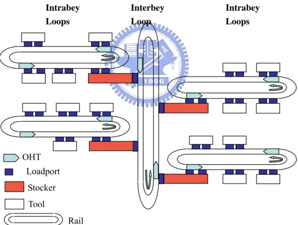
A typical AMHS system combines with one interbay loop and several intrabay loops [6], [8], [9]. Each loop has three major components, OHT, track and stocker. OHT is the lot carrier. It carries lot from bay to bay. The track is the path of OHT moving direction. The stocker is the storage buffer for lots to wait for next process. Figure 1 show the top view of an AMHS system configuration.
Figure 1. Top View of An OHT Configuration
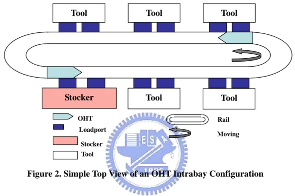
An OHT intrabay loop includes the collection of rails, OHTs, and load ports that are parts of process tools. The OHT is a kind of vehicle with grabber in the bottom. When a lot need to be moved, the OHT will go by the track to arrive right above the lot, lowing down the grabber, picking up the lot carrier, moving to the assigned
OHT Rail Intrabey Loops Interbey Loop Intrabey Loops Loadport Stocker Tool
destination, then depositing the lot carrier down. All OHT will be continuously moving following the same direction even they are empty, excluding they are doing hoisting works. The load ports are the interfaces where carries are picked up or delivered from and to production equipment as well as storage stockers. A load port can be uni-directional (either for input or output) or bi-directional (both for input and output). A typical OHT intrabay loop is, therefore, designated as a simple directed graph as depicted in Figure 2.
Figure 2. Simple Top View of an OHT Intrabay Configuration
2.2 AMHS Researches in 300mm Semiconductor Manufacturing
Many research efforts have been devoted to the automation of material handling systems in both 300mm interbay and intrabay [7], [10], [11], [12], [13], [14], [15]. Most of them focus on the design concept for effective integration of fab layout and AMHS in 300mm semiconductor manufacturing.
2.2.1 System Selection
Some of the researchers focus on layout of AMHS, and what kind of transport system should be suggested [16]. Lin et al. [17] explore wafer movements by using different types of vehicles between and within bays. Various combinations among four types of vehicles are discussed. They develop a mathematical model to determine the minimum number of vehicles for connecting transports.
2.2.2 Interbay Control
Cardarelli and Pelagagge [18] develop a simulation tool for design and management optimization of automatic interbay material handling and storage
Tool Tool Tool
Tool Tool Stocker OHT Rail Loadport Stocker Tool Moving
systems in wafer fabs. They use generalized probability density functions which are fitted with the observations from monthly historical data in a wafer fab as the scenarios to evaluate the dynamics of interbay material handling and storage systems. With respect to dispatching rules applied in a wafer fab, several heuristic dispatching rules, combined with direction selection, workcentre-initiated, and job-initiated dispatching, are simulated in the bi-directional interbay loop [19]. This paper concluded that the dispatching rule has a significant impact on average transport time, throughput, waiting time and vehicle utilization. The combination of SD-NV and FEFS (Shortest Distance, Nearest Vehicle, First Come First Serve) outperformed the other rules.
2.2.3 Intrabay Control
To achieve fab-wide transport optimization, Liao develops a management and control framework for prioritized automated material handling services [20]. Fu and Liao [21] propose an effective OHT dispatch policy, Modified Nearest Job First (MNJF), to achieve high throughputs while reducing the carrier delivery times in a single OHT loop. Kuo [22] develop a modular-based colored time Petri net (CTPN) to model the dynamic behavior of the OHT. An object-based simulation technique is used to determine the number of OHT vehicles in the planning stage and to control the dispatching in the operational stage.
2.2.4 Controls combined with Interbay and Intrabay
Liao and Fu propose an effective OHT dispatching polices to reduce the vehicle delivery time [23]. Lin et al [24] analyzes the performance of the connecting transport automated material handling system (AMHS) in a water fab. A two-phase experimental approach evaluates the connecting transport. The optimum combination of different methods can be obtained with a mixture of experiment.
2.2.5 Hot Lots Related
It is well known that lots of high priority has a significant impact on cycle time and throughput of regular production [25]. Ehteshami et al. [26] conduct object-oriented simulation experiments of a wafer fabrication model to investigate the impact of hot lots on cycle time of other lots in the system. Their simulation results show that as the proportion of hot lots in the wafer-in-process (WIP) increases, both the average cycle time and the corresponding standard deviation for all other lots increase. They conclude that hot lots induce either deterioration in the services for normal lots or an increase in inventory costs. Fronckowiak et al. [27] use a simulation tool, ManSim/X, to analyze the impact for different hot lot distributions for two different products. Narahari and Khan [28] model semiconductor manufacturing systems as re-entrant lines and study the effect of hot lots through an approximation
analysis of the re-entrant line model using mean value analysis (MVA). The results indicate that hot lots impose significant effects on mean and variance of cycle times, as well as throughput rate of normal lots. The MVA approximation is under the assumption of steady-state conditions. All of these researches focus on the wafer processing operations only, and none of them discuss the problems of hot lot effects on transport operations.
2.3 AGV Related Researches
The AGV (Automatic Guide Vehicle) system is very similar to OHT system. It plays an important role in tradition fabrication.
2.3.1 Comparison between AGV and OHT
Different from AGV, OHT is implemented on the overhead tracks. AGV system will occupy the floor space such that human operators cannot do operations in the same space. Instead, OHT system has the advantage of space utilization. Different from the popular 200mm AMHS solutions of OHS (Over Head Shuttle) and AGV (Automatic Guided Vehicle), it is very difficult to implement mechanisms of shortcut and bypass in an OHT intrabay loop because:
1. the length of an intrabay loop is shorter than that of an interbay.
2. at least four OHT service points (loadports) have to be replaced in order to add one pair of shortcuts.
3. at least two service points are needed for each bypass.
All of these may reduce the number of loadports, as well as that of processing equipment to be installed within a loop. This reduction of processing equipment will result in lower utilization in the expensive cleanroom space and is ineffective in fab layout design.
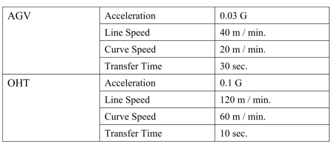
In addition to the space utilization, the speed of an OHT vehicle is faster than an AGV. The speed specifications of these two automation methods are tabulated in Table 2 [28]. According to the specification, the line speed of an OHT vehicle is more faster than that of AGV. OHT provides more high throughput, no vehicles congestion, and no any throughput impact by human working in fab, when executes the moving jobs. On the other hand, the fixed tracks provide fewer layout feasibility and more difficult maintenance.
Table 2. Comparison between AGV and OHT
Acceleration 0.03 G
Line Speed 40 m / min. Curve Speed 20 m / min. AGV
Transfer Time 30 sec.
Acceleration 0.1 G
Line Speed 120 m / min. Curve Speed 60 m / min. OHT
Transfer Time 10 sec.
2.3.2 Layout Configurations
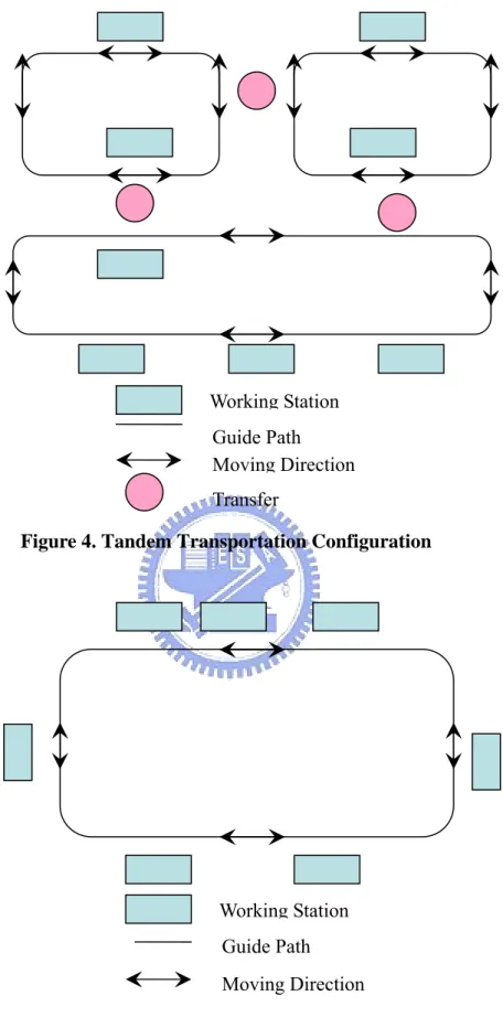
There are three major types of AGV layout configurations: single-loop [29], [30], tandem [31], [32], [33], and network. The single-loop system is the basic element of tandem. Several independent single loops construct the tandem system and connecting single loops compose the network system. The figure 3, 4 and 5 shows the concept configuration for network, tandem and single-loop, respective. Tachoco and Sinriech investigate the placing of single loop stations and let the vehicles traverse the loop in a fixed unidirectional sequence [29]. Tandem AGV structure was proposed in [32], which is routed with non-crossed circular loops. The throughput is more competitive in tandem AGV structure than the conventional structure [31].
Figure 3. Network Transportation Configuration
Working Station Guide Path Moving Direction
Figure 4. Tandem Transportation Configuration
Figure 5. Single-loop Transportation Configuration
For individual interbay and intrabay loop, they are both similar to uni-direction single-loop system with multiple vehicles, but the entire AMHS can be perceived as a
Working Station Guide Path Moving Direction Working Station Guide Path Moving Direction Transfer
tandem system.
2.3.3 Guide Path Directions
Kim and Tanchoco [34] define 4 major guide path directions for AGV system. There are:
1. Uni-directional. 2. Multiple-lane. 3. Bi-directional. 4. Mixed model.
The control logic of uni-direction is easier and cost is also cheaper [35]. Others types are complicated and difficult to control when number of vehicles increases. In semiconductor fab, a uni-directional guide with single lane is popular used for AMHS environment.
2.3.4 Vehicle Amount
Several researchers focus on number of required vehicles. Maxwell and Muckstadt [36] propose a time independent mathematical model to find out the minimum number of vehicles required in a given system. Their criterion is to minimize total traveling time for empty vehicles. Newton [37] determines vehicle number by simulating with two different dispatching rules: VLFW (Vehicle Looks For Work) and FIFO (First In First Out). Lin [38] proposes a FORTRAN computer program for vehicle number. He transforms the problem to minimum cost flow problem and using out-of-kilter algorithm to solve it.
2.3.5 Vehicle Scheduling
Time window concept is used for vehicle scheduling. Kim and Tanchoco [39] present an algorithm for finding conflict-free shortest-time routes for automated guided vehicles moving on a bi-directional flow network. A list of time occupied windows is reserved by scheduled vehicles and a list of free time windows is available for vehicles to be scheduled. Liu and Shen [40] solve several insertion-based savings heuristics for the fleet size and mix vehicle routing problem with time window constraints. The construction parameter yielded very good results.
2.3.6 Traffic Control
In order to prevent the blocking, collision, and deadlock, the traffic control is needed. The path segments are often subdivided into several non-overlapping zones and only one vehicle is permitted within a zone at the same time. Lee et al [41] propose a two-staged traffic control to ensure the collision free and reduced the transfer time. The Routing Table Generator (RTG) is used to find out the candidate
paths off-line, and then the On-line Traffic Controller (OTC) seeks the routing table to generate the transfer time motions. Hsieh and Lin [42] use Petri-Net to design a three stages system concept. The union of four basic path substructures (line, divide, merge, and intersection) can be used to construct a collision free zone. Bypass system [35] is another concept of traffic control. When a vehicle arrive its destination, it enters the bypass in front of the station. Meanwhile, the other vehicles can still run on the main path. Liu and Hung [30] control strategy to achieve the objectives: avoid shop deadlocks. A job shop manufacturing system with a single multi-load automated guided vehicle, which traverses around a single-loop guide path, is considered in this work. The efficiency of the proposed vehicle control strategy and the other two expanded strategies under various parameter designs are verified by computer simulation.
2.3.7 Automated Storage / Retrieval System (ASRS)
Five major topics are focused by pass researchers [43]:
1. operation control issues of S/RM (Storage / Retrieval Machine). 2. storage location issues.
3. retrieval location issues. 4. dwell-point location issues. 5. request sequencing issues.
The most popular rules for location assignment are RaNDoM assignment (RNDM), pattern search, Lowest Tier First (LFT), Shortest Processing Time (SPT) and turnover rate based ZONE assignment (ZONE) [44].
2.3.8 Multiple-load Vehicle
Multiple-load vehicle can reduce the total single-load vehicle number, but increase the control difficulty of system. Lee et al. [45] design several rules and use simulation to find that FP (Fixed-route-Part-priority rule) and VP (Variable-route-Part-priority rule) have good performances. Liu and Hung [30] propose a job shop manufacturing system with a single multi-load automated guided vehicle, which traverses around a single-loop guide path, is considered in this work.
2.3.9 Vehicle Dispatching
The vehicle dispatching rules take significant effects on system performance. The functionality of an AGV is very similar to OHT, thus, the AGV dispatching rules can be also applied to AMHS environment.
In previous AGV research, Egbelu and Tanchoco present two kinds of vehicle dispatching rules [46]. They design five work center initiated rules and seven vehicle initiated rules. The work center initiated rules are:
1. Random Vehicle (RV) rule. 2. Nearest Vehicle (NV) rule. 3. Farthest Vehicle (FV) rule. 4. Longest Idle Vehicle (LVI) rule. 5. Least Utilized Vehicle (LUV) rule.
On the other hand, the vehicle initiated rules includes: 1. Random Workcenter (RW) rule.
2. Shortest Travel Time / Distance (STT/D) rule. 3. Longest Travel Time / Distance (LTT/D) rule. 4. Maximum Outgoing Queue Size (MOQS) rule.
5. Minimum Remaining Outgoing Queue Space (MRQS) rule. 6. Modified First Come-first Serve (MFCFS).
7. Unit Load Shop Arrival Time (ULSAT) rule.
They claimed that the combination of the Nearest Vehicle (NV) rule and First Encounter First Serve (FEFS) rule is the best policy for AGV system to maximize throughput.
Egbelu [47] propose a demand driven rule (DEMD) for Just In Time (JIT) manufacturing system. Liu and Duh [48] present a heuristic rule by considering both distance and queuing length. Lin [49] applied the bidding concept to dispatching system. It provides a high flexibility and intelligence in control logic selection. Occena and Yokota [50] impalement a rule which focuses on inventory and transport control in JIT environment. Yim and Linn [51] use push based and pull based rule for vehicle initiated consideration. The results show that both rule performed well in term of average output rate. Lee [52] adds a tie-breaking idea into composite dispatching rule.
2.3.10 Vehicle Delivery Time
Most of researches use simulation method to calculate lot delivery time [23],[53],[54]. Simulation is always challenged, because it needs lots of running time and many model assumptions and simplifying realistic model. However, Shen and Lau [55] propose a two-phase model, which regards the AGV system network as a graph consisting of nodes connected by a set of arcs, and the AGV system as an M/G/N queueing system for free-ranging AGVs. Phase I, which is an integer programming-based approach, determines the minimum number of vehicles required to satisfy the system designer's specification on waiting time. Phase II, a heuristic rule-based approach, is to find a flow path which gives the least overall expected waiting time and service time. Liao et al. [56] present a neural-network-based
approach for prediction of average delivery times of lots that move in one intrabay loop in 300 mm AMHS.
CHAPTER
3
PREEMPTIVE
PRIORITY
POLICY
(PPP)
This chapter reveals the realistic issue of 300mm transportation of hot lots, then proposes the PPP method to solve this problem.
3.1 Problem Disclosure
In contemporary 200mm semiconductor foundry manufacturing, Operations of hot lots can be either preemptive against normal lots operations, or capacity-reserved for no-wait services. The hot lots are specially handled and carried by human operators to reduce the transport delay between distant processing equipment. However, it becomes very challenging to reduce the transport delay in 300mm automatic transport environments. In a 300mm foundry fab, frequently lots blocking happens within the intraby. Since the OHT moving speed is fast, when OHT exercises a hoisting work, the other OHTs after the hoisting one will be blocked. Let us find one example. From realistic data of one Taiwan fab, the OHT speed is around 2 meters per second. The hoisting time is 16 seconds. When the OHT doing the hoisting work, other OHT within 32 meters (16seconds * 2 meters per second) behind it will be block. Normally, one intrabay loop length is around 80 meter and will have 3 to 5 OHT in one intrabay. The regular loading of one intrabay moves is around 120 to 200. This means OHT system need to execute two or 3 moves per second. Obviously, frequently blocking can not be avoided. This issue is a big impact for the delivery time of hot lots.
3.2 Preemptive Priority Policy (PPP)
Intuitively, a lot with higher priority should enjoy its privilege of transportation against those with lower priority. Among a given set of transport lots, an empty OHT will serve first the lot with the highest priority. Observing the empirical human operations for carrying hot lots and considering the effect and limitation from OHT transportation, we propose a heuristic OHT dispatching method to expedite the movement of the hot lots in order to avoid any blocking due to normal lots.
Define a transport job as a macro of transfer commands. It was contained that:
1. A request for an empty OHT is initialized for carrier transfer from the departure to the destination.
2. An empty OHT arrives and picks up the carrier at the departure. 3. The OHT moves the carrier from the departure to the destination. 4. The OHT deposits the carrier down at the destination.
OHT delivery time is then defined as the time to complete a transport job. The OHT dispatching is an assignment of a transport job to an empty OHT. The dispatched OHT is reserved to the job once after it is dispatched and becomes empty again after completing this job. The objective of OHT dispatching is to minimize OHT delivery time.
Given a set of transport jobs ready for and waiting to be transferred by OHTs, an empty OHT is dispatched to the job of highest priority and the transportation of the OHT is preemptive. That is, once an empty OHT is dispatched to the highest priority job, any other ongoing transport operations which may block the transportation of this OHT will be pending until its job completes. Figure 7 shows the major concepts of PPP.
The heuristic algorithm is designed in detail as below. 1. Overall Rule
Step 1
The OHT always follows the “first meet, first serve” on transport jobs. An empty OHT is dispatched to the job, which’s nearest to the current location of the empty OHT.
Step 2
If a hot lot job is issued, follow the hot lot rule. 2. Hot Lot Rule
Step 1
The AMHS controller checks the location of all empty OHTs. Reserve the nearest empty OHT to execute this job.
Step 2
Even an empty OHT is reserved for a hot lot job, if another empty OHT happens and closer the lot than original reserved OHT, change the reservation to nearest OHT.
Step 3
If no any empty OHT, AMHS controller waits, until the first empty OHT happened. Then AMHS controller reserves the only one empty OHT to execute that job.
Step 4
loading, aborts the job, if there is a hot lot reserved OHT or OHTs with hot lot is coming in rear of the distance D. D is equal to the average moving speed * one lot hoisting time. By following the realistic data, the average speed is 2 meter/second and hoisting time is 16 seconds. So, D is 32 meters.
Step 5
When an OHT with normal lot job is ready for unloading, aborts the job, if there is a hot lot reserved OHT or OHTs with hot lot is coming in rear of the distance D.
Step 6
If more than one hot lot jobs happen, follow the first hot lot meet, first hot lot serve.
Step 7
CHAPTER
4
MODULARIZED
SIMULATON
METHOD
(MSM)
The problems of lot delivery are dressed and MSM are developed to estimate the lot delivery time in 300 AMHS environment.
4.1 Problem Formulation
In fab operations, scheduling is the major impact factor of tools capacity allocation, tools utilization control and bottleneck management. However, there is no any effective method to estimate delivery time in 300mm automatic material handling systems (AMHS) operation.
Define a transport job as a macro of transfer operations including:
1. A request for transport to an empty OHT for a lot from its departure (current location) to the destination (location for next process step). 2. An empty OHT arrives and picks up the lot at the departure.
3. The OHT moves the lot from the departure to the destination. 4. The OHT delivers the lot at the destination.
Define lot delivery time as the time to complete a transport job. Lot delivery time is composed of theoretical transport time, waiting time, OHT hoisting time, blocking time, and loop switching time.
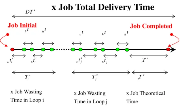
We define the some notations before formulating the delivery time forecast problems in 300mm OHT systems. Figure 6 shows the relationship of time notation.
Figure 6. The Relationship of Time Notations
Some assumptions are made as follows. Lots move from one loop to the other via a loop switch mechanism in a stocker. All vehicles in a loop reside in the same loop during the time horizon. Loop loading is assumed to be unchanged during the time horizon. Since the acceleration and deceleration of each OHT operation are relatively small, they are thus neglected. There are no failures and maintenance activities on all the entities during the simulation horizon. The inter-arrival time of transport jobs is assumed to be of exponential distribution. Furthermore, as the stocker serves as the only gateway between this loop and others, infinite capacity of each stocker is assumed.
Our objective is to estimate the total delivery time (D ) of lots. The total x
delivery time (D ) of job x includes waiting time, theoretical time, blocking time in x
all the loops it passes, twice hoisting time for loading and unloading (τ ), and loop switching time (η). Assume that transport operations are loop-independent. That is, transport operations in one loop are independent of those in the other loops. Based on this assumption on loop independence, we can add all the transport time in each individual loop to calculate D . That is, x
. ) ( 2 ) (w b U τ j iη D xl xl j i l xl x =
∑
+ + + + − = (1)where the departure of job x is in loop i and the destination in loop j.
Assume that delivery times in each loop are independent and normal distribution. For a job, the variance of its delivery time is equal to the sum of all the variances in each loop along its moving path. If we take the α risk level, the upper bond of
Job Initial
x DT x i wt t h t c x j wt x tT t h x Job Wasting Time in Loop i x Job Wasting Time in Loop jx Job Total Delivery Time
x i bt x j bt x i T Tjx t h t h x Job Theoretical Time x tT
Job Completed
confidence value can be calculated as following:
∑
= − + j i l l x z s D 1α 2 (2)where the probability Pr(Z ≥z1−α)=α,α∈R and s is the variance of l2 delivery time in loop l.
4.2 Modularized Simulation Method (MSM)
Due to the complicated fab dynamics, it is almost impossible to solve for the exact solution to Dx in equation (1). In practical applications, people are most
interested in determining the average and variances of delivery time of a job. Instead, we adopt computer simulation techniques to obtain these statistics. However, it is either too complex to model the sophisticated fab operations as well as the whole AMHS; or too much time-consuming to simulate with a full-scaled fab model. We, therefore, propose a heuristic approach to decompose the complicated problem into small ones. Ideas of our modularized simulation method (MSM) are described as follows:
Rather than building the sophisticated model of a 300mm fab, we utilize the features of loop configuration in 300mm OHT systems. We then decompose the whole 300mm AMHS into several independent loops, from which we develop simulation models for each loop. As the operations of each loop are independent, the average loop waiting times can be additive, so do the blocking times. The average delivery time of a job can be estimated by adding all the waiting and blocking times in each loop along its transport path, as described in equation (3).
, ) ( 2 ) ( ] [D W B U τ j iη E l xl j i l l x =
∑
+ + + + − = (3)where Wl and Bl are statistics calculated with simulation results.
Observing the dynamics of the OHT system, system loading is one of the factors to cause resource contention. The increased population of hot lots will impose long time delays on the normal lots. As the number of OHTs increase, system performance usually gets improved due to the increased resources. We, therefore, consider three dominating control variables for discrete simulation method for an OHT loop -- loading ratio (ρ), population of hot lots (Ω), and the number of OHTs (υ) in the loop. The models of each individual OHT loop are simulated for various combinations of OHT vehicles, loop loading, and percentage of hot lots.
variance of its lot waiting time and blocking time can be calculated. Nonlinear multiple regression technique is then used to estimate these variables.
The loop variance can be estimated by the sum of mean square errors due to waiting and blocking. That is, the standard deviation sl is equal
to
∑
− + j i l l l MSEB MSEW ) ( 2 2 .CHAPTER
5
EXPERIMENT
DESIGN
The chapter first describes the simulation environment and then detail dresses the experiment models for both PPP method and MSM method.
5.1 Simulation Environment
To convey our idea in estimating lot transport times in 300mm AMHS, simulation experiments are conducted based on realistic data from a local 300mm fab. Our simulation models are implemented with the discrete-event simulation package -- eM-PlantTM from Tecnomatix Technologies Ltd. All the experiments are executed
in a Pentium-III personal computer with Microsoft Windows XP. The eM-PlantTM is
an object-oriented simulation system with characteristics of hierarchy, inheritance, and concurrency. There are some built-in objects in there for easy development. Users can easily modify them into user-defined objects for their specific purposes. Some of the objects defined in our simulation models are depicted in Table 3.
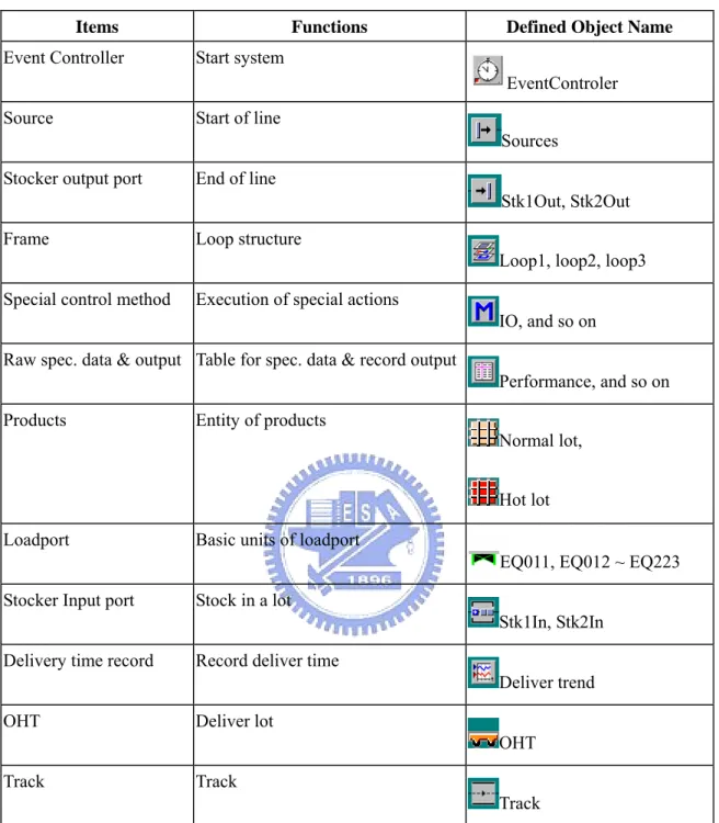
The Chapter 5.2 and 5.3 have some same assumptions. The running speed of an OHT is set to 2 meters per second. The time for each loading/unloading operation of a carrier is 16 seconds, respectively. Since the acceleration and deceleration of each OHT operation are relatively small, they are thus neglected. Because the reliability is not our focus on this study, we assume that there are no failures and maintenance activities on all the entities during the simulation horizon. Since we are interested in the effects on the performance of the OHT system, the from-to relationship between two processing tools is adopted, instead of considering the whole process flow of a semiconductor product. The inter-arrival time of transport events is probabilistic and is assumed to be of exponential distribution. For simplifying the simulation model, stockers of infinite capacity are assumed. No matter the capacity of stocks, the stocks perform an inter-medium of loops and the hot lots only pass through them.
Table 3. Objects in the eM-Plant Simulation Model
Items Functions Defined Object Name
Event Controller Start system
EventControler Source Start of line
Sources Stocker output port End of line
Stk1Out, Stk2Out
Frame Loop structure
Loop1, loop2, loop3 Special control method Execution of special actions
IO, and so on Raw spec. data & output Table for spec. data & record output
Performance, and so on Products Entity of products
Normal lot, Hot lot Loadport Basic units of loadport
EQ011, EQ012 ~ EQ223 Stocker Input port Stock in a lot
Stk1In, Stk2In Delivery time record Record deliver time
Deliver trend
OHT Deliver lot
OHT Track Track
Track
5.2 PPP Simulation Model
In the simulation models, we consider an OHT loop in 79.4 meters long, where there are two stockers and 23 pieces of equipment. In order to study the impact due to the hot lots rule, a non-differentiated rule, Nearest Job First (NJF) rule, is adopted for the comparison. The NJF rule utilizes the straightforward idea of first meet, first serve and it has been suggested as a good dispatching rule in many AGV applications [21], [47].
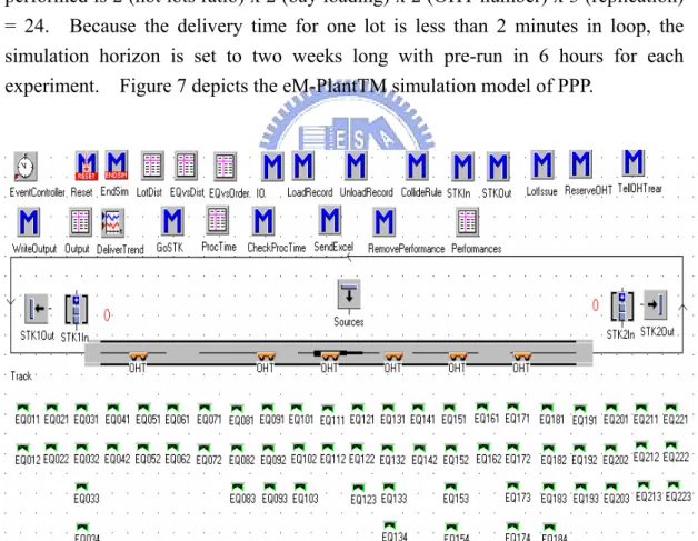
consider three dominating control variables -- loading ratio (ρ), population of hot lots (Ω), and the number of OHTs (υ) in the loop. Systems with heavy loadings are adopted to highlight the effect of the hot lot rule in resource contention. Two loading ratios, 100% and 90% of the design specification, are used in the simulation. As the increasing hot lots population will impose long time delays on the normal lots drastically, two distributions of hot lots, 2% and 8%, are designed for the tests. As the number of OHTs increase, system performance usually gets improved due to the increased resources. In the simulation study, we consider two configurations of the OHT numbers, 4 and 6 OHTs in the loop, respectively. Eight simulation experiments are then conducted based on the scenarios for these three control variables. The OHT delivery time, the time from the birth of a job to its completion, is considered as the performance measure. We design each experiment is simulated for three times. The total number of simulation experiments performed is 2 (hot lots ratio) x 2 (bay loading) x 2 (OHT number) x 3 (replication) = 24. Because the delivery time for one lot is less than 2 minutes in loop, the simulation horizon is set to two weeks long with pre-run in 6 hours for each experiment. Figure 7 depicts the eM-PlantTM simulation model of PPP.
Figure 7. eM-PlantTM Simulation Model of PPP
5.3 MSM Simulation Model
The only performance measure in our simulation model is the lot delivery time. Inputs to the simulation system include loop loading, percentage of hot lots and
number of vehicles in each loop. Without loss of generality, we build an OHT system with three loops as the control scenario, which represents the tool-to-tool transportation through several loops. Assume that all the lots in the simulation start from loop 1, and transit to loop 2, and then move to loop 3, and finally leave the system. Figure 8 shows the conceptual simulation model. The simulation horizon is set to two weeks long with time units in seconds after a warm-up of 6 hours.
Figure 8. A 3-OHT-Loops Model
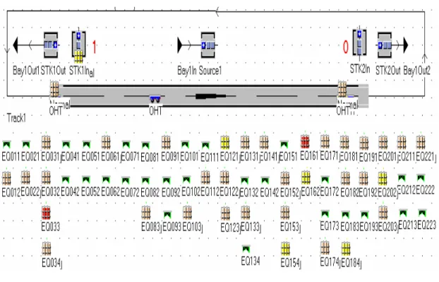
Figure 9 demonstrates the simulation model of loop 1. In our simulation, each subsystem has the similar structure, but with different parameter settings for process tools. Each OHT loop is in 79.4 meters long, where there are two stockers and 23 pieces of equipment. All loops are designated with the same tool configurations. Loops 1 and 2 have the same processing capacity of 97.2 lots per hours, and 94.2 lots for loop 3 per hours. The loop switching time is set to 16 seconds. Here, we adopt the PPP policy as the OHT dispatching rule for all loops in our simulation experiments. The PPP policy dispatched an empty OHT to a job with the highest priority. The dispatched OHT is reserved to the job once after it is dispatched and becomes empty again after completing this job. Our objective of OHT dispatching is to minimize the carrier delivery times. For each OHT loop, the OHT dispatching rule deployed for this loop remains unchanged.
Figure 9. OHT Loop Simulation Model
The models of each individual OHT loop are simulated for various combinations of OHT vehicles, loop loading, and percentage of hot lots to collect the statistics of waiting time and blocking time for each loop. Seven loop loading ratios (ρ), 90%, 92.5%, 95%, 97.5%, 100%, 102.5%, and 105% of the design specifications, are used in the simulation. Five configurations of hot lot percentage (Ω), 2%, 4%, 6%, 8% and 10%, are designed for the hot lot population tests. In the simulation study, we consider three configurations of the number of OHT vehicles (υ), 3, 4 and 5 OHTs in the loop. One hundred and five simulation experiments (ρ:7, Ω:5, υ:3, 7*5*3=105) are then conducted based on the scenarios for these three control factors.
CHAPTER
6
SIMULATION
RESULTS
AND
ANALYSIS
Detail experiment results of PPP and MSM are demonstrated in this chapter. Results analysis are proposed.
6.1 PPP Simulation Results
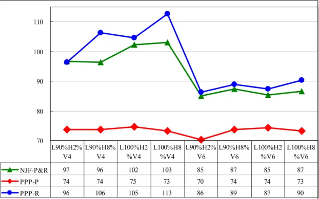
The results of experiment are demonstrated on table 4. Since NJF rule has no capability to distinguish the movement for lots with different priorities, the results of both hot lots and normal lots are all the same in different configurations. In the average results of each configuration, we find that the PPP performs well comparing with NJF in hot lots. Figure 10 demonstrates the comparison of average results in different configurations.
Table 4. Average Experiment Results in OHT Delivery Time (in seconds) PPP
System Configuration NJF
Hot Lots Normal Lots
Bay Loading Hot Ratio # of OHT Mean Standard Deviation Mean Standard Deviation Mean Standard Deviation 90% 2% 4 97 10 74 27 96 20 90% 8% 4 96 10 74 35 106 21 100% 2% 4 102 10 75 23 105 18 100% 8% 4 103 10 73 33 113 20 90% 2% 6 85 9 70 34 86 17 90% 8% 6 87 9 74 36 89 19 100% 2% 6 85 9 74 37 87 18 100% 8% 6 87 9 73 38 90 21 Average 93 10 73 33 97 19
Remarks: 1. R is the abbreviation of normal lots. 2. P is the abbreviation of hot lots. 3. M is the abbreviation of Mean.
70 80 90 100 110 NJF-P&R 97 96 102 103 85 87 85 87 PPP-P 74 74 75 73 70 74 74 73 PPP-R 96 106 105 113 86 89 87 90 L90%H2% V4 L90%H8% V4 L100%H2 %V4 L100%H8 %V4 L90%H2% V6 L90%H8% V6 L100%H2 %V6 L100%H8 %V6
Remarks: 1. NJF–P&R is the item of NJF hot lots and normal lots (same results). 2. PPP-P is the item of PPP hot lots.
3. PPP-R is the item of PPP normal lots. 4. L is the abbreviation of bay loading. 5. H is the abbreviation of hot lots percentage. 6. V is the abbreviation of OHT vehicle number.
Figure 10. Simulation Average Results in Different Configurations (in seconds)
Compare with NJF and PPP rules by statistics testing, the average transport time of hot lots has significant difference. The total number of simulation experiments performed is 2 (hot lots ratio) x 2 (bay loading) x 2 (OHT number) x 3 (replication) = 24. Therefore, n is equal to 24. The alpha value is set to 0.05. Table 5 depicts the results of testing. The t value is 12.78. Table 6 shows the comparison of normal lots, the t value is -1.54. This means the transport time of two methods has no significant difference.
Table 5. Method Comparison for Hot Lots T-Tests
Variable Method Variances DF t Value Pr > |t|
time Satterthwaite Unequal 24.6 12.78 <.0001
Equality of Variances
Variable Method Num DF Den DF F Value Pr > F
time Folded F 23 23 28.32 <.0001
Table 6. Method Comparison for Normal Lots T-Tests
Variable Method Variances DF t Value Pr > |t|
time Pooled Equal 46 -1.54 0.1316
Equality of Variances
Variable Method Num DF Den DF F Value Pr > F
time Folded F 23 23 1.73 0.1984
Obviously, The PPP do expedite the delivery time of hot lots but result in longer delivery time of normal lots in both mean and its standard deviation. The PPP rule is thus considered effective in reducing OHT delivery time of hot lots. In these scenarios, the average theoretical OHT delivery time (time without suffering any transport delay) is 52 seconds. The delay time (waiting time and blocking time) by NJF is 93 - 52 = 41 and 73 – 52 = 21 by PPP. In average, the delay time of hot lots can be reduced by 49% (from 41 sec. to 21 sec.) for PPP rules. These transport delays are caused by the waiting time before an empty OHT picks up the hot lots. Even longer average delivery time of normal lots is incurred in both mean and standard deviation.
The major orders of 300mm fab is 130nm logic Cu flow with 36 masks with five 193nm levels. We summary average lot cycle time data from one Taiwan 300mm fab. See table 7. Using PPP, the average cycle of 130mm can be efficiently reduced around 4.45 days. The results have been verified by some 300mm fab managers. The consequences are affirmative.
Table 7. Hot Lots Performance Improvement by PPP
Characteristics Value
130nm logic layer 36 layers
Average cycle time/per layer 0.83 day
Average cycle time 29.88 days
Average theatrical process time 12.43 days Average holding time (28% of cycle
time)
8.37 days
Average waiting time 9.08 days
PPP average improved time (49% waiting time)
4.45 days
PPP average cycle time 25.43 days
PPP average cycle time / per layer 0.71 days
6.2 MSM Simulation Results
We first check the correlation of variables in each loop, which are number of vehicles, percentage of hot lots, and loop loading of the loop. Since loops 1 and 2 have the same processing capacity, the correlation results of these two loops are listed in Table 8. For loop 3, its correlation results are showed in Table 9. Note that all correlation coefficients are less than 0.05, which implies that these variables are almost independent. Thus, the multicollinearity effect in regression modeling is not considered.
Table 8. Variables Correlation Table of Loops 1 and 2
Pearson Correlation Coefficients, N = 105
ρ Ω υ
ρ 1.00000 -0.03197 -0.02973
Ω -0.03197 1.00000 -0.00820
Table 9. Variables Correlation Table of Loop 3
Pearson Correlation Coefficients, N = 105
ρ Ω υ
ρ 1.00000 0.00084 -0.04079
Ω 0.00084 1.00000 0.01098
υ -0.04079 0.01098 1.00000
In order to satisfy the assumptions of normality and homoscedasticity of variables, all the data in the simulation model are first standardized before regression. The nonlinear multiple regression technique is then used to determine the characteristics among the variables.
As some of the values are fixed and mandatory for both normal lots and hot lots transports, only the non-value-added ones are considered in our numerical analysis to concentrate on the comparisons. Here, define job non-value-added time to be the sum of job waiting time and carrying blocking time along the loops.
The regression model of each loop is estimated. Tables 10 and 11 demonstrate the regression equation models of hot and normal lots transports, perspective. For hot lots, the r squares of estimated waiting time of loops 1, 2 and 3 are 0.9240, 0.9240 and 0.9359, respectively. The r squares of estimated blocking time of loops 1, 2 and 3 are 0.7085, 0.7085 and, 0.7664, respectively. Among the cases of normal lots, 19 scenarios are diverged and thus excluded. The r squares of estimated waiting time for loop 1, 2 and 3 are 0.9962, 0.9962 and 0.9464, respectively. The r squares of estimated blocking time for loops 1, 2 and 3 are 0.9926, 0.9926 and, 0.8952, respectively. From the above data, we find that the r squares of waiting time perform well. All of them are larger than 0.9. The r squares of blocking time are not as good as those for the waiting time. However, its minimum value is 0.7085. It is still good. We therefore conclude that the estimation results are sound for realistic data.
Table 10. Hot lots Regression Equation Models Loop 1 & 2 Waiting Time Loop 1 & 2 Blocking Time Loop 3 Waiting Time Loop 3 Blocking Time Intercept 21.50159 0.6337154 20.2206 0.3778069 ρ -1.48846 0.1269775 - -Ω 1.05056 - 1.58692 0.1023634 υ - - -3.76146 -ρ2 - - 0.47758 0.1164286 Ω2 - -0.066419 - -υ2 1.1691 0.2898994 1.45006 0.3488951 ρ3 1.07716 - - -υ3 -2.88357 -0.1551079 - -ρυ - - -0.28075 -ρΩ2 1.61559 - - -ρυ2 - 0.1386985 - 0.2285595 ρΩ3 - - -0.18441 -ρυ3 - -0.0793121 0.25466 -0.3313136 ρ2Ω - - -0.32692 -ρ2υ 0.3853 0.132838 - 0.0539166 ρ2Ω3 - 0.0480561 - -ρ3υ -0.20039 - - -ρ3Ω2 -0.73747 - - -ρ3υ3 - - 0.1105681 Ωυ - - -0.63611 -Ω2υ -0.28723 - - -Ω3υ -0.18302 - - 0.026031169 ρΩυ2 - -0.0543073 - -ρΩυ3 - - - 0.037815072 ρΩυ - 0.1043169 -
-Table 11. Normal lots Regression Equation Models Loop 1 & 2 Waiting Time Loop 1 & 2 Blocking Time Loop 3 Waiting Time Loop 3 Blocking Time Intercept 81.32562 5.8673664 51.67604 5.724393 Ω - 0.8280088 -39.83946 0.7978134 υ2 145.62597 -0.6955856 57.11975 -0.6210066 υ3 -153.42675 1.0888534 -61.0485 0.8614784 ρυ -357.54335 - - 0.5169598 ρυ2 294.37959 - 75.74651 -0.1971796 ρΩ3 - - - 0.0771256 ρυ3 - 0.1808086 -79.46953 -ρ2Ω - - 41.34817 -ρ2Ω2 -21.34325 - - -ρ2υ2 132.74628 - 86.29826 -ρ2υ3 -96.62153 -0.09095 -66.96296 -ρ3υ2 - - 38.70043 -ρ3υ3 - - -27.07322 -0.1015002 Ωυ2 147.91911 - 99.83647 -Ωυ3 -119.36141 0.1575254 -75.86935 0.212823 Ω2υ2 45.00707 - 25.43009 -Ω2υ3 -26.90771 - -16.64411 -ρΩυ2 111.16575 - 92.69853 -ρΩυ3 -90.88981 - -66.18869 -ρΩ2υ2 - - 15.72335 -ρΩ3υ - -0.09095 -
-Tables 12and 13 demonstrate the simulation results for 105 scenarios for hot and normal lots, respectively. We find that the dominating factor is the number of OHT vehicles. The effects from different combinations of loading and hot lot ratio are not significant. Even though loop loading is higher than 100%, it seems not to reach the maximum capacity of the OHT system for hot lots. Its OHT non-value-added time is still acceptable. However, for normal lots, when the loop loading is high and the vehicles are scarce (e.g., number of vehicles is 3), the results become diverged. This is caused by the PPP, from which the transport of hot lots are preemptive. When the numbers of OHT is not sufficient, normal lots will not receive enough resources to serve for them. Their delivery times then become diverged. It also trends to have longer delivery time if the loading is high. That is,
the more hot lot ratio is, the longer delivery time incurs. In average, the means of non-value-added time of priority jobs are 69.9 seconds for MSM and 70.1 seconds for simulation results, respectively. The average difference is just 0.2 second. The standard deviations of prioritized delivery time are 13.9 seconds and 13.4 seconds, respectively. After removing diverged outliers, the means of non-value-added time of normal lots are 239.5 seconds for MSM and 239.4 seconds for simulation results, respectively. The standard deviations of regular delivery time are 189.8 seconds and 190.3 seconds, respectively. Complying with our conjecture on the effect of forecasting methods in all of the scenarios tested, the MSM and system simulation results are very close. These results are coincided with our expectation. The results show that the MSM is a good method to estimate the delivery time in 300mm OHT environment. Moreover, the system run time for MSM in 1st time needs 2days, but we can acquire the equations of each loop. Therefore, we only need less than 1 min. to acquire lot delivery time for other times. But, the simulation method costs 7 days for the results every time. The results also have been verified by some 300mm fab managers. The consequences are affirmative, too.
Table 12. Non-Valuable Times Comparisons for Hot lots Non-Value-Added Time
Number of Vehicles Configuration
Modularized Simulation Method Simulation Results
Loading Priority Ratio 3 4 5 3 4 5
2% 70.0 57.1 53.8 74.0 57.7 53.1 4% 73.5 60.7 55.8 76.0 62.0 53.9 6% 77.7 62.7 57.3 72.0 62.0 57.8 8% 81.5 65.4 58.9 83.0 66.0 58.1 90% 10% 83.3 68.0 60.4 80.0 64.0 59.8 2% 74.7 57.3 49.4 71.0 57.1 50.2 4% 81.2 63.7 56.1 80.0 63.0 55.5 6% 85.2 66.4 59.4 83.0 64.0 57.9 8% 88.8 68.6 59.2 85.0 66.0 81.0 92.5% 10% 91.2 67.8 57.9 95.0 69.0 62.0 2% 77.0 59.1 50.8 77.0 59.3 50.2 4% 81.6 63.4 56.0 77.0 64.0 55.2 6% 87.7 65.7 58.4 87.0 64.0 59.2 8% 89.3 67.4 58.9 97.0 69.0 58.3 95% 10% 93.4 67.4 56.7 94.0 66.0 57.3 2% 80.9 59.8 51.2 77.0 59.7 53.0 4% 85.0 61.6 53.9 84.0 62.0 53.1 6% 86.9 64.6 56.6 86.0 70.0 56.9 8% 90.7 66.9 57.6 93.0 64.0 62.0 97.5% 10% 97.6 68.8 58.7 97.0 67.0 62.0 2% 85.0 61.5 53.7 86.2 64.0 52.4 4% 85.3 61.9 53.8 87.0 60.0 57.9 6% 87.6 64.1 55.2 92.0 67.0 59.2 8% 90.2 68.4 57.4 88.0 73.0 59.1 100% 10% 98.5 70.6 61.0 92.0 72.0 65.0 2% 88.1 63.8 56.9 91.0 59.5 53.9 4% 88.3 63.4 56.5 86.0 66.0 58.1 6% 89.0 64.7 56.3 89.0 70.0 56.3 8% 93.0 67.2 59.4 92.0 71.0 62.0 102.5% 10% 101.3 73.1 61.2 99.0 74.0 61.0 2% 90.5 64.2 56.5 85.0 63.0 55.8 4% 93.7 68.2 55.9 93.0 61.0 57.0 6% 94.2 70.5 58.0 90.0 70.0 59.8 8% 98.3 70.9 60.6 94.0 72.0 64.0 105% 10% 100.1 73.3 62.2 94.0 75.0 63.0 Mean 69.9 70.1 Summary Std. Deviation 13.9 13.4
Table 13. Non-Valuable Times Comparisons for Normal lots Non-Value-Added Time
Number of Vehicles Configuration
Modularized Simulation Method Simulation Results
Loading Priority Ratio 3 4 5 3 4 5
2% 314.5 146.0 123.0 334.0 140.0 117.0 4% 380.9 144.0 118.3 373.0 149.0 116.0 6% 391.4 152.3 122.9 404.0 159.0 124.0 8% 480.2 161.1 127.9 471.0 164.0 127.0 90% 10% 497.1 165.5 128.7 484.0 173.0 134.0 2% 395.9 143.9 111.1 397.0 147.0 113.0 4% 482.7 154.5 118.5 493.0 160.0 119.0 6% 554.0 166.6 126.9 549.0 165.0 130.0 8% 667.9 179.3 134.1 675.0 177.0 137.0 92.5% 10% 949.8 184.1 140.5 976.0 182.0 138.0 2% 498.7 153.5 112.8 485.0 157.0 117.0 4% 595.2 165.1 123.2 551.0 167.0 124.0 6% 772.9 173.5 131.2 801.0 178.0 133.0 8% 872.8 186.7 135.1 830.0 184.0 132.0 95% 10% X 200.1 144.2 X 190.0 139.0 2% 677.4 163.5 115.5 700.0 164.0 119.0 4% 881.4 170.5 123.4 890.0 168.0 127.0 6% X 186.0 135.0 X 187.0 134.0 8% X 197.1 140.1 X 190.0 134.0 97.5% 10% X 206.2 145.5 X 197.0 146.0 2% X 177.1 121.6 X 169.0 119.0 4% X 182.4 127.1 X 174.0 128.0 6% X 198.1 133.2 X 201.0 138.0 8% X 216.1 141.6 X 215.0 139.0 100% 10% X 221.6 152.8 X 220.0 158.0 2% X 177.2 124.9 X 177.0 123.0 4% X 192.9 130.3 X 187.0 130.0 6% X 207.5 134.1 X 204.0 133.0 8% X 221.2 145.6 X 211.0 143.0 102.5% 10% X 247.2 153.6 X 263.0 155.0 2% X 179.0 123.0 X 185.0 124.0 4% X 201.1 130.4 X 202.0 127.0 6% X 220.2 138.9 X 226.0 141.0 8% X 239.7 150.0 X 244.0 148.0 105% 10% X 275.4 159.0 X 280.0 159.0 Mean 239.5 239.4 Summary Std. Deviation 189.8 190.3