分類技術與貝氏網路之應用---法學文件之語意標記與人機互動之使用者建模

行政院國家科學委員會專題研究計畫 成果報告

分類技術與貝氏網路之應用：法學文件之語意標記與人機互

動之使用者建模

計畫類別： 個別型計畫

計畫編號： NSC94-2213-E-004-008-

執行期間： 94 年 08 月 01 日至 95 年 10 月 31 日

執行單位： 國立政治大學資訊科學系

計畫主持人： 劉昭麟

計畫參與人員： 黃珮雯、鄭人豪、陳禹勳及林仁祥

報告類型： 精簡報告

報告附件： 出席國際會議研究心得報告及發表論文

處理方式： 本計畫可公開查詢

中 華 民 國 95 年 10 月 4 日

行政院國家科學委員會補助專題研究計畫 出國報告

分類技術與貝氏網路之應用：

法學文件之語意標記與人機互動之使用

計畫類別：■ 個別型計畫 □ 整合型計畫

計畫編號：NSC 98－2213－E-004－008

執行期間： 94 年 8 月 1 日至 95 年 10 月 31 日

計畫主持人：劉昭麟

共同主持人：

計畫參與人員： 黃珮雯、鄭人豪、陳禹勳及林仁祥

成果報告類型(依經費核定清單規定繳交)：■精簡報告 □完整報告

本成果報告包括以下應繳交之附件：

□赴國外出差或研習心得報告一份

□赴大陸地區出差或研習心得報告一份

■出席國際學術會議心得報告及發表之論文各一份

□國際合作研究計畫國外研究報告書一份

處理方式：除產學合作研究計畫、提升產業技術及人才培育研究計畫、

列管計畫及下列情形者外，得立即公開查詢

□涉及專利或其他智慧財產權，□一年□二年後可公開查詢

執行單位：國立政治大學 資訊科學系

中 華 民 國 95 年 10 月 4 日

Abstract

We report the research work for investigating the annotation of judicial documents in

Chinese and applying Bayesian networks for student modeling. This piece of work embarked in

the year 2005 and will continue toward 2008. We have achieved reasonable results in the first

year.

Overview

In the past many years, we have studied classification techniques for categorizing judicial

documents in Chinese. The categorization of judicial documents can be useful in practice if we

can achieve satisfactory accuracy. Although we hope, the actual application of our system may

not take place in the courts. With our current achievements, we see that we can build a

Google-like server for judicial consultation. The main difference between our system and Google

will be that we do not require users to choose and type in key words for search. In a normal

prosecution procedure, the defendant will receive a prosecution document from the courts. To

know that the prosecution documents are about, the users just feed the whole file to our system to

search similar prior documents. Our system can provide prior documents that are similar to the

current document based on prosecution reasons or legal articles that might be cited for the current

case.

In addition to the categorization of judicial documents, we have also attempted to apply

machine learning-based methods for learning student models. The input data to our learners are

simulated students’ records for taking tests. We implemented the simulator in the past year, and

are continuing to improve it. Given students’ test records, our classifier try to tell how students

learning composite concepts. We have identified some key issues in this research direction, and

expect to work on them in the continued projects. At this moment, we see that there are chances

that computers can help educational experts to select detailed models about students’ learning

patterns. However, this is not a simple work, particularly when students’ test records do not

deterministically reflect students’ competence.

Technical skeletons

Since we have applied very different approaches for the document classification and student

modeling problems in our research, we have to provide the skeletons separately.

Classification of judicial documents

As in the work that we did in the past many years, we applied k nearest neighbor (kNN)

methods for the classification task. With a preprocessing procedure, we extracted key information

from the documents and converted them into a set of features. In applying kNNs, we calculated

the similarity between two documents with the similarity measure defined based on the feature

sets.

In the past, we have been using word-based features in our work. A Chinese word is a

sequence of characters that we segmented from a normal Chinese text. In our research that took

place between 2004 and 2005, we have applied the introspective learning method to adjust the

weights for the keywords, hoping to improve the accuracy of our classifiers.

This year, we switched to phrase-based features. The hunch is that using phrases, consisting

of two words, should make the phrase more specific in their semantics, and hopefully can

improve the effectiveness of our classifiers. The creation and weighting of the phrases and the

evaluation of our methods had been reported in an international conference. Please be referred to

the appended paper for more details.

Student modeling with Bayesian networks

We believe that what reported in this summary is a brand new issue that one can find in the

literature. We will make a great contribution to the world, if this research direction eventually

leads to real world applications.

How do we know how students learn composite concepts? When a composite concept

consists of multiple basic concepts, there can be many different ways to learn it. For instance,

there are at least 14 different ways to learn a composite concept that contains four basic concepts.

(Please see the appended papers for reasons.) A human teacher may believe that s/he knows how

her/his students learn. However, such beliefs are generally not critically verified. We do not

intend to disregard human intuition, but we believe that machines can be useful in searching for

the real learning process.

We organize our work into several components. Since this is the first step of our study, we

do not have data for real students yet. Instead, we implemented a student simulator that is

structurally similar to a computer-assisted student assessment system. The simulator can generate

students’ test records, which will be used in the place of test records of real students.

Given the student records, we employed several classification techniques to guess the

learning patterns. In running the simulator, we had to provide key information about students’

learning patterns so that the simulator can create test records accordingly. Such key information

was known to us but was not provided to our classifiers. Hence, our classifiers had to guess these

hidden learning patterns.

The details of how we conducted the experiments are provided in the appended papers. It is

found that our classifiers can hit the current answer, if the experimental settings are favorable.

However, the problem is not as easy as it may appear, and our classifiers performed not clearly

better than a random guesser when the settings are really unfavorable.

Published papers

Since we have conducted quite a lot of work in a year, we thought it might be more direct to

provide the papers that we published and presented in international conferences for both the NSC

reviewers and the ordinary public to know more about our achievements.

We have published our papers in AI and IEEE conferences. We provided the list, and the

papers follow.

„ C.-L. Liu. Learning students' learning patterns with support vector machines, Lecture

Notes in Computer Science 4203: Proceedings of the Sixteenth International

Symposium on Methodologies for Intelligent Systems (ISMIS’06), 601-611. Bari, Bari,

Italy, 27-29 September 2006. (SCIE)

„ C.-L. Liu and C.-D. Hsieh. Exploring phrase-based classification of judicial documents

for criminal charges in Chinese, Lecture Notes in Computer Science 4203: Proceedings

of the Sixteenth International Symposium on Methodologies for Intelligent Systems

(ISMIS’06), 681-690. Bari, Bari, Italy, 27-29 September 2006. (SCIE)

Proceedings of the Sixth IEEE International Conference on Advanced Learning

Technologies (ICALT’06), 187-189. Kerkrade, Limburg, Netherlands, 5-7 July 2006.

(EI?)

„ C.-L. Liu. Learning how students learn with Bayes nets, Lecture Notes in Computer

Science 4053: Proceedings of the Eighth International Conference on Intelligent

Tutoring Systems (ITS’06), 772-774. Jhongli, Taiwan, 26-30 June 2006. (SCIE)

Learning Students’ Learning Patterns with Support

Vector Machines

Chao-Lin Liu

Department of Computer Science, National Chengchi University, Taiwan [email protected]

Abstract. Using Bayesian networks as the representation language for student

modeling has become a common practice. Many computer-assisted learning systems rely exclusively on human experts to provide information for con-structing the network structures, however. We explore the possibility of apply-ing mutual information-based heuristics and support vector machines to learn how students learn composite concepts, based on students’ item responses to test items. The problem is challenging because it is well known that students’ performances in taking tests do not reflect their competences faithfully. Ex-perimental results indicate that the difficulty of identifying the true learning patterns varies with the degree of uncertainty in the relationship between stu-dents’ performances in tests and their abilities in concepts. When the degree of uncertainty is moderate, it is possible to infer the unobservable learning pat-terns from students’ external performances with computational techniques.

1 Introduction

Providing satisfactory interaction between human and machines requires good com-putational models of human behaviors. Take computer-adaptive testing (CAT) for example. Researchers build models based on the Item-Response Theory (IRT) [1,2] and Concept Maps [3] for predicting students’ performances and selecting appropri-ate test items for assessment. With good student models, a computational system can evaluate students’ competence with less test items than traditional paper-and-pencil tests will need, and can achieve better accuracy in its evaluation. In addition, test takers can access a CAT system almost any time at any location, and can obtain their scores on the spot. Hence, CAT has been adopted in many official evaluation activi-ties, including TOFEL and GRE, although there are sporadic criticisms [4].

Typically, domain experts provide information about student models, which are then implemented with computational techniques. CAT systems that adopt IRT as-sume that a student’s responses to test items are mutually independent given the stu-dent’s competence, so IRT-based systems generally take the so-called naïve Bayes models [5, 6]. Based on this assumption, the problem of building student models boils down to learning the model parameters from observed data [7, 8]. Similarly, Liu et al. assume the availability of concept maps of students and teachers, and design algo-rithms for comparing the concept maps for assessment [3].

Although human experts can choose good models from candidate models, they may not agree on their choices. For instance, Millán and Pérez-de-la-Cruz discussed a hierarchical structure of Bayesian networks [9] that included nodes for subjects,

top-ics, concepts, and questions [10]. Vomlel employed nodes for skills and misconcep-tions, and used relevant nodes as direct parents of nodes for tasks [11].

In this paper, we explore computational techniques for comparing the candidate models for students. Although we do not expect computational techniques will give better model structures than human experts will do in the short term, we hope that computational techniques can assist human experts to identify more precise models. More specifically, we would like to guess how students learn composite concepts. A

composite concept results from students’ integration of multiple basic concepts. Let dABC denote the composite concept that involves three basic concepts cA, cB, and cC.

How do we know how students learn the composite concept? Do they learn dABC by directly integrating the three basic concepts, or do they first integrate cA and cB into an intermediate product, say dAB, and then integrate dAB with cC?

We compare candidate models that are represented with Bayesian networks, based on students’ responses to test items. Students’ responses to test items reflect their competences in the tested concepts in an indirect and uncertain manner. The relation-ship is uncertain because students may make inadvertent errors and luckily hit the correct answers. We refer to these situations as slip and guess, respectively, hence-forth. Slip and guess are frequently cited in the literature, and many researchers adopted Bayesian networks to capture the uncertainty in their CAT system, e.g., [6, 8, 10-12].

As a result, our target problem is an instance of learning Bayesian networks. This is not a new research problem, and a good tutorial is already available [13]. However, learning Bayesian networks for student modeling is relatively rare, based on our knowledge, particularly when we would try to induce a network directly from stu-dents’ item responses. Vomlel created network structures from stustu-dents’ data and applied principles provided by experts to refine the structures [11]. Besides those difficulties for learning structures from data, learning a Bayesian network from stu-dents’ data is more difficult because most of the variables of interests are not directly observable. Hence, the problem involves not just missing values and not just one or two hidden variables.

In our experiments, we have 15 basic and composite concepts. We cannot observe whether students are competent in these concepts directly, though we assume that we can collect students’ responses to test items that are related to these concepts. The problem of determining how students learn composite concepts is equivalent to learn-ing the structure of the hidden variables given students’ item responses.

We propose mutual information (MI) [14] based heuristics, and apply the heuris-tics for predicting the hidden structures in two ways: a direct application and training support vector machines (SVMs) [15] for the prediction task. Experimental results indicate that it is possible to figure out the hidden structures under moderate uncer-tainty between students’ item responses and students’ competence.

We provide more background information in Section 2, introduce the MI-based heuristics in Section 3, present the SVM-based method in Section 4, and wrap up this paper with a discussion in Section 5.

2 Preliminaries

We provide more formal definitions, explain the source of the simulated students’ item responses, and analyze the difficulties of the target task in this section.

The goal of our work is to find the hidden structure of the unobservable nodes that represent students’ competence in concepts, based on observed students’ item re-sponses. We assume that students learn composite concepts from parent concepts that do not have overlapping basic concepts. For the problem of investigating how stu-dents learn dABC that we mentioned in Section 1, we assume that there are four pos-sible answers: AB_C, AC_B, BC_A, and A_B_C, where the underscores separate the parent concepts. Although there is no good reason to exclude a learning pattern like

AB_BC, including such overlapping parent concepts will dramatically make the

prob-lem more complex. We obtained students’ item responses from a simulation program that was reported in a previous work [6]. In this paper, we will try to learn how stu-dents learn dABCD, and there are 14 possible ways to learn this target concept.

2.1 Creating Simulated Students

Although not using real students’ data subjects our work to criticisms, we believe that, if we can employ computational models to predict students’ behaviors in CAT sys-tems, we should believe that the same computational model is trustworthy for simu-lating students’ behaviors. The use of simulated students is not our invention, previ-ous and well-known work has taken the same approach for studying computational methods, e.g., [10, 12].

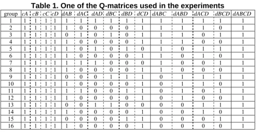
Using Liu’s simulator that is described in [6], we can control the structure of the Bayesian network and the generation of the conditional probability tables (CPTs). The generation of the CPTs relies on a random number generator that uniformly sam-ples numbers from a given range. In order to specify competence patterns of the stu-dent population, we also have to provide a matrix that is similar to the Q-matrix [16], and Table 1 shows the matrix that we used in many of our experiments. The columns are concepts, and the rows are student groups. When the column is a basic concept, cells are 1 if a typical student in the student group is competent in the concept, and cells are 0 otherwise. When the column is a composite concept, cells are 1 if a typical student in the student group is able to integrate the parent concepts to form the com-posite concept if s/he is competent in the parent concepts. Although the cells are ei-ther 0 or 1, Liu employed random numbers to give an uncertain relationship between

Table 1. One of the Q-matrices used in the experiments

group cA cB cC cD dAB dAC dAD dBC dBD dCD dABC dABD dACD dBCD dABCD 1 1 1 1 1 1 1 1 1 1 1 1 1 1 1 1 2 1 1 1 1 1 0 0 0 0 1 1 1 1 0 1 3 1 1 1 1 0 1 0 1 0 1 1 1 0 1 1 4 1 1 1 1 1 0 0 0 0 1 1 1 0 0 1 5 1 1 1 1 1 0 1 0 1 0 1 0 1 1 1 6 1 1 1 1 1 0 0 0 0 1 1 0 1 0 1 7 1 1 1 1 1 1 1 0 0 0 1 0 0 1 1 8 1 1 1 1 1 0 0 0 0 1 1 0 0 0 1 9 1 1 1 1 0 0 0 1 1 1 0 1 1 1 1 10 1 1 1 1 1 0 0 0 0 1 0 1 1 0 1 11 1 1 1 1 1 1 0 0 1 1 0 1 0 1 1 12 1 1 1 1 1 0 0 0 0 1 0 1 0 0 1 13 1 1 1 1 0 0 1 1 0 0 0 0 1 1 1 14 1 1 1 1 1 0 0 0 0 1 0 0 1 0 1 15 1 1 1 1 0 0 0 0 1 1 0 0 0 1 1 16 1 1 1 1 1 0 0 0 0 1 0 0 0 0 1

student groups and compe-tence in concepts through a simulation parameter:

groupInfluence. A student’s

behavior may deviate from his/her typical group compe-tence pattern with a probabil-ity that is uniformly sampled from the range [0, groupInfluence].

We assumed that every concept had three test items in the experiments, and the network shown in Figure 1 shows a possible network when we consider the problem in which there are only three basic concepts. Note that in this network, we assume that students learn dABC by directly integrating the three basic concepts, which is indicated by the direct links from the basic concepts to the node labeled dABC. We cannot show the network for the case in which there are four basic concepts in this paper, due to the size of the network. (There will be 15 nodes for concepts, 3×15 nodes for test items, and a lot more links between these 60 nodes.)

The probabilities of slip and guess are also controlled by a simulation parameter:

fuzziness. Students of a student group may deviate from the typical behavior with a

probability that is uniformly sampled from [0, fuzziness].

Given the network structure, the Q-matrix, and the simulation parameters, we can create simulated students. In our experiments, we assumed that a student can belong to any of the 16 student groups with equal probabilities. Following Liu’s strategy, we used a random number, ρ that was sampled from [0, 1] to determine whether a stu-dent would respond to a test item correctly or incorrectly. The conditional probability of correctly responding to a test item given a student belonged to a particular group can be calculated easily with Bayesian networks. Consider the instance for iA1, a test item for cA. If ρ is smaller than Pr(iA1=correct|group=g₁) when we simulated a student who belonged to the first group, we assumed that this student responded to

iA1 correctly. Since there were 15 concepts, a record for a simulated student would

contain the correctness for each of 45 (=3×15) test items.

After using the networks to create simulated students, we hid the networks from our programs that took as input the item responses and guessed the structures of the hidden networks.

2.2 Contents of the Q-Matrix and Problem Complexity

The contents of the Q-matrix influence the prior distributions of students’ competence patterns and the performance of simulated students [12]. Clearly, there can be many different ways to set the contents of the matrix.

We set the Q-matrix in Table 1, partially based on our experience. Notice that all columns for the basic concepts and the target concept, dABCD, are 1. This should be considered a normal choice. If we do want to learn how students learn dABCD, we should try to recruit students who appear to be competent in dABCD to participate in our experiments. In addition, there is no good reason to recruit anyone who is not competent in any of the basic concepts in the experiments. We set the values for

dABC, dABD, dACD, and dBCD to 16 possible combinations, and this is why we

group

cA cB cC

dAB dBC dAC dABC

iA1 iA3 iA2 iC2 iC3 iC1 iB2 iB3 iB1

iAB1 iAB2 iAB3

iABC1 iABC2 iABC3

iAC3 iAC2 iAC1 iBC3 iBC2 iBC1

include 16 student groups in Table 1. We randomly choose the values of dXY, where

X and Y are symbols for basic concepts, and will report experimental results for other

possible settings.

When we consider β basic concepts in the problem, the number of possible ways to learn how students learn a composite concept that is comprised of all these β con-cepts is related to the Stirling number of the second kind [17]. It is easy to verify that this number grows rapidly with β, and we will have 14 alternatives if we set β to 4.

∑

∑

3 MI-Based Heuristics

Consider the situation when we generate students’ data from the network shown in Figure 1. If we have the true states of all the concept nodes, it is not difficult to learn the network structure with a variant of the PC algorithm [18] implemented in Hugin [19]. However, we cannot observe the true competence levels of students in reality, and can only indirectly measure the competence through the results of examinations. Moreover, the item responses do not perfectly reflect students’ competence, due to many reasons including guess and slip. Hence, we need to find indirect evidence that may help us to predict the hidden structure.

3.1 Estimating the MI Measures

Recall that we have assumed that every simulated student will respond to three test items for each concept. Out of three test items, a student may correctly respond to 0%, 33%, 67%, and 100% of the test items. Hence, it is possible to estimate the state of the concept nodes with the percentage of correct responses. We can also use the per-centages to estimate the state of a set of variables. For instance, Pr(cA=33%, cB=66%) can be the percentage of students who correctly respond to exactly one item for cA

and two items for cB. Given such estimates, we will be able to compute the mutual

information between any two sets of variables, and apply the estimated mutual infor-mation in guessing the hidden structure.

Intuitively, the variables that are more closely re-lated to each other will exhibit higher mutual in-formation. Partial networks shown in Figure 2 include five possible ways to learn

dABCD, i.e., A_B_CD,

AB_C_D, ACD_B, ABD_C, and A_B_C_D. Let MI(X;Y) denote the mutual

informa-tion between two sets of variables, X and Y. If A_B_CD is the true structure, we ex-pect that it is more likely for the estimated MI(cA, cB, dCD; dABCD) to be larger than the estimated MI(dAB, cC, cD; dABCD) and other estimated MI measures. Hence, we can employ the following heuristics.

Heuristics: The structure that has the largest estimated MI measure is the hidden

structure. dABCD dCD cD cA cB cC dABCD dACD cD cA cB cC dABCD dAB cD cA cB cC dABCD cD cA cB cC dABCD dABD cD cA cB cC

Before we estimate the MI measures, we add 0.001 to the number of occur-rences of every possible combination of variables. This will avoid the zero probability problems, and is a typical smoothing procedure for estimating probability values [20].

3.2 Experimental Evaluation

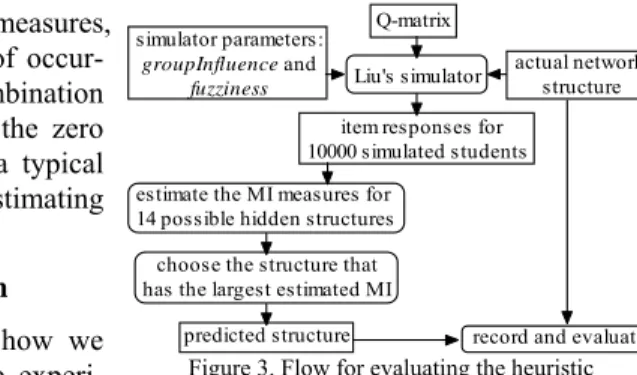
Figure 3 shows the flow of how we evaluated the heuristic. In the

experi-ments, we used five different network structures to create simulated students, and their main differences are shown in Figure 2. The parent concepts of other composite concepts that do not appear in the sub-networks in Figure 2 are the basic concepts. For instance, the parent concepts of dABD in the network that used the leftmost sub-network in the top row of Figure 2 are cA, cB, and cD. As we mentioned in Section 2, we mainly used the Q-matrix in Table 1 in our experiments. We set groupInfluence and fuzziness to different values in {0.05, 0.1, 0.15, 0.2, 0.25, 0.3}, so there were 36 combinations. We did not try values larger than 0.3 because they were beyond con-sideration normally discussed in the literature. For each of the five network structures and a combination of groupInfluence and fuzziness, we sampled 600 network in-stances with the Q-matrix shown in Table 1, and created a different population of 10000 simulated students for each of these instances. The choice of “10000” was arbitrary, and the goal was to make each of the 16 groups include many students.

An experiment corresponded to a different combination of groupInfluence and

fuzziness, so there were 36 experiments. We used accuracy to measure the quality of

our prediction of the hidden structures. It was defined as the percentage of correct prediction of 3000 (=5×600) randomly sampled network instances that were used to create the simulated students. According to Equation (1), there were 14 possible an-swers when β is 4. Hence, to guess the hidden structure of each of these 3000 net-work instances, we calculated the estimated MI measures for 14 possible answers from the item responses of the 10000 simulated students.

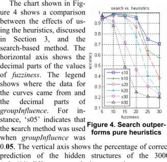
Figure 4 summarizes the ex-perimental results. The vertical axis shows the accuracy, the hori-zontal axis shows the decimal part of fuzziness, and the legends mark the values of groupInfluence used in the experiments. Curves in these charts show a general trend that we expected. Increasing the values of

groupInfluence and fuzziness made

the relationship between students’ item responses and their compe-tence patterns more uncertain and our prediction less accurate. When

Figure 4. Accuracy achieved by the MI-based heuristics

Q-matrix Liu's simulator

estimate the MI measures for 14 possible hidden structures

item responses for 10000 simulated students

predicted structure record and evaluate actual network

structure

choose the structure that has the largest estimated MI simulator parameters:

groupInfluence and fuzziness

both groupInfluence and fuzziness were both close to 0.3, the accuracy was about 0.2. It is easy to interpret 0.2 as a result of random guesses from five possible answers, but this is not correct. Although we used only five network structures that are shown in Figure 2 to create simulated students, our prediction program did not take this into account, and could consider network structures that were not included in Figure 2. The fact is that our heuristics favored particular structures, which we learned by look-ing into the internal data collected in experiments. When both groupInfluence and

fuzziness were large, the heuristics tended to favor A_B_C_D, which happened to be

one of the true answers. As a result, we had the accuracy of 0.2. Had we excluded

A_B_C_D from the true networks, the accuracy would become smaller than 0.2.

Although we expected that the accuracy should improve as we reduced the values of groupInfluence and fuzziness, the experimental results did not fully support this intuition. (When we conducted experiments for the cases in which there were only three basic concepts, experimental results did support this intuitive expectation.) When both groupInfluence and fuzziness were close to 0.05, the heuristics tended to favor AB_CD against other competing structures, making the accuracy worse than we expected. More specifically, we created a 14×14 confusion matrix [20] and found that our heuristics chose AB_CD relatively frequently when the true structures were

A_B_CD and AB_C_D. The accuracy could hit as low as 0.85 when both groupInflu-ence and fuzziness were both 0.05 for other Q-matrices that were different from the

Q-matrix shown in Table 1. These Q-matrices were different in the settings in the

dXY columns, where both X and Y represents a basic concept. This phenomenon is

certainly not desirable, though understandable, because of the similarity between and

A_B_CD, AB_C_D, and AB_CD.

When the heuristics led us to choose a wrong structure, the estimated MI measures for the chosen structures were not larger than the MI measures for the correct struc-tures by a big margin. In fact, we found that, when the heuristics failed to choose the correct answers, most of the estimated MI measures were very close to each other. Hence, we expect that if we consider the ratios between the estimated MI measures, we may design more effective heuristics. We included ratios between estimated meas-ures as featmeas-ures for building the SVM-based classifiers that we report below.

4 SVM-based Methods

Support vector machines [15] are a relatively new formalism that can be applied to the task of classifications. We can train SVMs with training patterns that are associated with known class labels, and the trained

SVMs can be used to predict the classes of test patterns. In this work, we employed the LIBSVM packages provided by Chang and Lin [21].

4.1 Preparing for Experiments

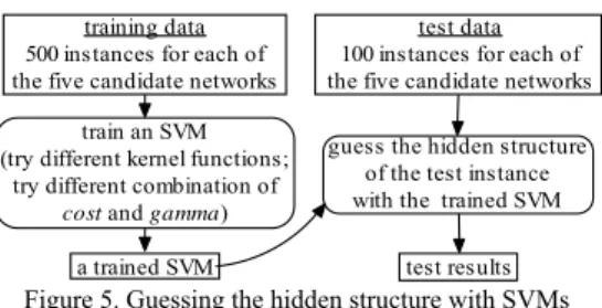
Figure 5 summarizes the main steps that we took to apply SVMs in our work. As explained in Section 3.2, we obtained students’ data in 36 different experiments. In

guess the hidden structure of the test instance with the trained SVM

test results a trained SVM

test data 100 instances for each of the five candidate networks training data

500 instances for each of the five candidate networks

train an SVM (try different kernel functions;

try different combination of

cost and gamma)

each of these experiments, there were 600 network instances for each of the candidate networks shown in Figure 2. Therefore, we used students’ data obtained from 500 network instances for each of the candidate network as the training data, and used the students’ data obtained from the remaining 100 network instances as the test data.

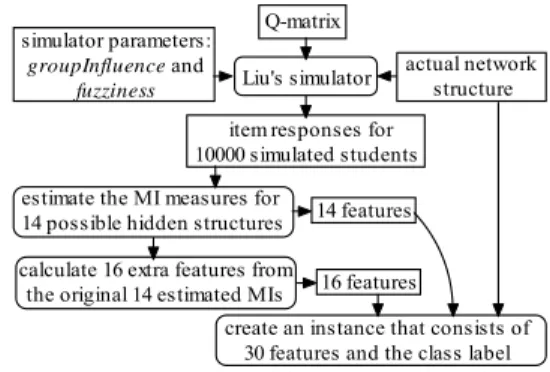
Figure 6 summarizes how we pre-pared the training and test instances. In addition to the original 14 esti-mated MI measures, we also com-puted ratios between the estimated MI measures as features. The introduction of ratios was inspired by analyses that we discussed at the end of Section 3.2. We divided the original 14 estimated MI measures by the largest estimated MI measure in each training instance. This gave us 14 new features. We also

divided the largest estimated MI measure by the second largest estimated MI measure, and divided the largest estimated MI measure by the average of all estimated MI measures. This gave us 2 more features, so we used 30 features for each of the 500 training instances for each of the five candidate networks. The true answers (also called class labels) were attached to the instances for both training and testing. In summary, we created a training instance from 10000 simulated students, and there were 2500 (=5×500) training instances, each with 30 attributes and a class label. When testing the trained SVMs, we produced the 16 extra features from the original 14 estimated MI measures for each of the test instances as well. The true answer was attached to the test instance so that we could compare the true and predicted answers, but the SVMs did not peek at the true answers.

4.2 Results

Charts shown in Figure 7 show the experimental results. The vertical axis, the hori-zontal axis, and the legend carry the same meanings as those for charts in Figure 4. The titles of the charts indicate what types of SVMs we used in the experiments. We used the c-SVC type of SVMs in all experiments, and tried three different kernel functions, including polynomial

(c-svm-poly), radial basis (c-svm-rb), and sigmoid (c-svm-sm) kernels. Among these tests, using polyno-mial and radial basis kernels gave almost the same accuracy, and both performed better than the sigmoid kernel. However, it took a longer time for us to train an SVM when we used the polynomial kernel.

Comparing the curves for the same experiments in Figures 3 and 4 show the significant

improve-Figure 7. Accuracy achieved by the SVM-based methods

Q-matrix Liu's simulator

estimate the MI measures for 14 possible hidden structures

item responses for 10000 simulated students actual network structure simulator parameters: groupInfluence and fuzziness

calculate 16 extra features from the original 14 estimated MIs

14 features 16 features

create an instance that consists of 30 features and the class label

ments achieved by using the SVMs. In the middle chart in Figure 7, the accuracy stays above 0.75 even when groupInfluence and fuzziness were 0.3. The heuristics-based method got only 0.2 in accuracy under the same situation. In addition, the trends of all curves support our intuitive expectation—larger groupInfluence and

fuzziness would lead to worse accuracy. The problem that occurred in the upper left

corners of the charts in Figure 4 was also gone. Even when we tried different Q-matrices, smaller groupInfluence and fuzziness also made the prediction of the hidden structure easier than when we used larger groupInfluence and fuzziness.

We have to explain that we had to search for the best parameters for SVMs when we trained SVMs. In particular, we ran experiments that used different values for cost and gamma in LIBSVM, using default values for other parameters. Different combi-nations of cost and gamma led to different accuracy in guessing the hidden structures for the test data. In our experiments we tried combinations of cost and gamma from values in {0.1, 0.2, …, 1.9}, and used the best accuracy for the test data in 381 (=19×19) cases when we prepared charts in Figure 7.

5 Concluding Remarks

We tackle a student modeling problem that requires us to infer the hidden model for learning composite concepts, based on observations of variables that have only indi-rect and uncertain relationships with variables in the hidden model. Experimental results indicate that this task is not impossible, and we can actually achieve good results when the situations are favorable.

We report results of two different approach—A heuristics-based and an SVM-based approach. Charts shown in Figures 3 and 7 clearly show that the SVM-SVM-based approach is more effective. However, the advantages of our SVM-based approach come at some costs. We will need experts to enumerate the candidate networks and guess the contents of the Q-matrix. Only after obtaining these information, can we create simulated students and train the SVMs, which will then be used to guess the hidden structure with students’ item responses. (Although we did not use item re-sponses of real students in our experiments, we will have to do so in reality.)

Though we cannot discuss all experimental results in this paper, our experience in-dicates that the contents of the Q-matrix affect the final accuracy. The contents of the Q-matrix show what types of students that we should recruit for investigating how the students learn the composite concepts. Results reported in this paper were acquired with the Q-matrices that assumed students were competent in dABCD and all basic concepts. If we allow cells in these columns to be zero, then the final accuracy will be affected. However, we do not think this should happen in reality. If we do want to learn how students learn dABCD, we should have tried as hard as possible to collect item responses from students who appear to be competent in dABCD and all basic concepts. Given the intentionally introduced uncertainties, i.e., groupInfluence and

fuzziness, our algorithm does allow errors in recruiting students, and experts do not

have to provide very exact information about the Q-matrices. The SVM-based ap-proach is reasonably robust in this aspect.

We hope the reported results can be useful for student modeling in reality. Our ex-perience underscores the importance of experts’ opinion for the success of the model-ing task. Experimental results also show the potential applicability of the

heuristics-based methods for selecting the correct hidden sub-structure even when experts’ opinions were not available.

Acknowledgements

This research was partially supported by contract NSC-94-2213-E-004-008 of the National Science Council of Taiwan. We gratefully thank the reviewers for their invaluable comments, and will answer their questions that we cannot do so in this page-limited paper during the oral presentation.

References

1. 1. W. J. van der Linden and C. A. W. Glas, Computerized Adaptive Testing : Theory and Practice, Kluwer, Dordrecht, Netherlands, 2000.

2. H. Wainer et al., Computer Adaptive Testing : A Primer, Lawrence Erlbaum Associates, NJ, USA, 2000.

3. C.-C. Liu, P.-H. Don, and C.-M. Tsai, “Assessment based on linkage patterns in concept maps,” J. of Information Science and Engineering, vol. 21, pp. 873–890, 2005.

4. G. Smith, “Does Computer-Adaptive Testing Make the Grade?” ABCNEWS.com, 17 March 2003. 5. R. J. Mislevy and R. G. Almond, “Graphical models and computerized adaptive testing,” CSE

Technical Report 434, CRESST/Educational Testing Services, NJ, USA, 1997.

6. C.-L. Liu, “Using mutual information for adaptive item comparison and student assessment,” J. of Educational Technology & Society, vol. 8, no. 4, pp. 100−119, 2005.

7. F. B. Baker, Item Response Theory : Paraemter Estimation Techniques, Marcel Dekker, NY, USA, 1992.

8. R. J. Mislevy, R. G. Almond, D. Yan, and L. S. Steinberg, “Bayes nets in educational assessment: Where do the numbers come from?” in Proc. of the Fifteenth Conf. on Uncertainty in Artificial Intelligence, pp. 437−446, 1999.

9. J. Pearl, Probabilistic Rasoning in Intelligent Systems : Networks of Plausible Inference, Morgan Kaufmann, CA, USA, 1988.

10. E. Millán and J. L. Pérez-de-la-Cruz, “A Bayesian diagnostic algorithm for student modeling and its evaluation,” User Modeling and User-Adapted Interaction, vol. 12, no. 2-3, pp. 281−330, 2002. 11. J. Vomlel, “Bayesian networks in educational testing,” Int. J. of Uncertainty, Fuzziness and

Knowledge-Based Systems, vol. 12, no. Supplement 1, pp. 83−100, 2004.

12. K. VanLehn, Z. Niu, S. Siler, and A. Gertner, “Student modeling from conventional test data : A Bayesian approach without priors,” Lecture Notes in Computer Science, vol. 1452, pp. 434−443, 1998. 13. D. Heckerman, “A tutorial on learning with Bayesin networks,” in M. I. Jordan (ed.), Learning in

Graphical Models, pp. 301−355, MIT Press, MA, USA, 1999.

14. T. M. Cover and J. A. Thomas, Elements of Information Theory, John Wiley & Sons, NY, USA, 1991. 15. C. Cortes and V. Vapnik, “Support-vector network,” Machine Learning, vol. 20, pp. 273−297, 1995. 16. K. K. Tatsuoka, “Toward an integration of item-response theory and cognitive error diagnoses,” in N.

Fredericksen et al. (eds.), Diagnostic Monitoring of Skill and Knowledge Acquisition, Erlbaum, NJ, USA, 1990.

17. D. E. Knuth, The Art of Computer Programming: Fundamental Algorithms, Addison-Wesley, MA, USA, 1973.

18. P. Spirtes, C. Glymour, and R. Scheines, Causation, Prediction, and Search, second edition, MIT Press, MA, USA, 2000.

19. Hugin: http://www.hugin.com

20. I. H. Witten and E. Frank, Data Mining: Practical Machine Learning Tools and Techniques, second edition, Morgan Kaufamnn, CA, USA, 2005.

21. C.-C. Chang and C.-J. Lin, LIBSVM: A library for support vector machines, 2001. http://www.csie.ntu.edu.tw/~cjlin/libsvm

Exploring Phrase-Based Classification of Judicial

Documents for Criminal Charges in Chinese

Chao-Lin Liu and Chwen-Dar Hsieh

Department of Computer Science, National Chengchi University, Taiwan [email protected]

Abstract. Phrases provide a better foundation for indexing and retrieving

documents than individual words. Constituents of phrases make other compo-nent words in the phrase less ambiguous than when the words appear separately. Intuitively, classifiers that employ phrases for indexing should perform better than those that use words. Although pioneers have explored the possibility of indexing English documents decades ago, there are relatively fewer similar at-tempts for Chinese documents, partially because segmenting Chinese text into words correctly is not easy already. We build a domain dependent word list with the help of Chien’s PAT tree-based method and HowNet, and use the re-sulting word list for defining relevant phrases for classifying Chinese judicial documents. Experimental results indicate that using phrases for indexing indeed allows us to classify judicial documents that are closely similar to each other. With a relatively more efficient algorithm, our classifier offers better perform-ances than those reported in related works.

1 Introduction

We investigate the effectiveness of applying phrases for indexing judicial docu-ments in Chinese. Conventional wisdom and experimental results suggest that phrases provide better indications of contents of the indexed documents than keywords, thereby offering better chances of higher quality of information retrieval. Indeed, many natural languages contain homonyms and polysemes, so using isolated key-words for indexing takes the risk of interpreting key-words as unintended senses, and using phrases helps to alleviate the ambiguity problems with the contextual informa-tion provided by the surrounding words. Due to this intuiinforma-tion, Salton, Yang and Yu have pioneered the applications of phrases for indexing English documents as early as 30 years ago [1], and many researchers have followed this line of work [2, 3].

Chinese text consists of Chinese characters, and a number of consecutive charac-ters form a word in the sense of English words. For instance, XUN ( ) and QI ( ) are two Chinese characters, and XUN-QI ( ) is a Chinese word approximately corresponding to weapons in English. SH-YONG-XUN-QI ( ) is a Chinese phrase that contains two words, where SH-YONG ( ) means use in English, and SH-YONG-XUN-QI means use weapons in English.

Partially due to our ignorance, we have not been able to identify sufficient work that is directly related to indexing Chinese documents with phrases. More commonly, people segment Chinese text with the help of a machine readable lexicon, and then index the documents with Chinese words. With special techniques for obtaining in-formation about Chinese words such as Chien’s PAT tree-based approach [4], one may segment Chinese text without using lexicons. Instead of going through Chinese word segmentation first, some have used character level bigrams for indexing Chi-nese documents [5, 6]. This approach offers a much improved performance than character-level indexing for Chinese text, while requiring a much larger space of index terms [7]. To further improve the quality of search results, some consider short Chinese words for indexing [7].

As an exploration toward phrase-based indexing of Chinese text, we consider word-level bigrams for indexing indictment documents in Chinese. To this end, we rely on both HowNet [8] and Chien’s PAT tree-based methods for identifying useful Chinese words. After obtaining definitions of Chinese words, we segment each document for obtaining pairs of words, and use them as the signatures of the docu-ments. We define the similarity between indictment documents based on the number of common term pairs. Having built this infrastructure, we classify indictment docu-ments based on their prosecution categories as Liu did in [9], and classify indictment documents based on their cited articles as Liu did in [10]. Current experimental re-sults indicate that using term pairs leads to classification of higher quality for the former task. However, the new method provides only comparable performance on the latter task. Our methods differ from Liu’s methods for the second task in two impor-tant ways. In addition to using different indexing units, i.e., single terms vs. term pairs, we use different ways to obtain weights for these indexing units. We are still looking into the second task for further improvements.

Section 2 provides more background information regarding our work. Section 3 discusses our methods of obtaining Chinese words for the legal domain from our corpus. Section 4 extends the discussion for how we obtain phrases, how we assign weights to the phrases, and how we use the phrases for comparing the similarity be-tween indictment documents. Section 5 contains the experimental results, and Section 6 wraps up this paper with some discussions.

2 Background

We provide more background information on details of our classification tasks. We exclude information how we segment Chinese character strings into word strings [9] for page limits. We follow a standard procedure for segmenting Chinese, i.e., prefer-ring the longer matches while using a lexicon to determine the word boundaries, that has been adopted in the literature.

We can classify indictment documents in two different levels of grain sizes. The coarser lever is based on the prosecution categories, and the more detailed level is based on the cited articles. We consider six different prosecution categories: larceny ( ), robbery ( ), robbery by threatening or disabling the victims ( ),

re-ceiving stolen property ( ), causing bodily harm ( ), and intimidation ( ). We use X1, X2, ..., X6, respectively, to denote these categories henceforth. The crimi-nal law in Taiwan dedicates one chapter to each of these prosecution reasons, except that the two types of robberies X2 and X3 occupy the same category.

Once judges determine the prosecution categories of the defendant, they have to decide what articles are applicable to the defendants. Each chapter for a prosecution category contains a few articles that describe applicability and corresponding sen-tence of the article. Not all prosecution categories require detailed articles that sub-categorize cases belonging to the prosecution category, but some prosecution catego-ries require more detailed specifications of the prosecutable behaviors than others. In this paper, we concern ourselves with articles 266, 267, and 268 for gambling ( ). Article 266 describes ordinary gambling cases, article 267 describes cases that in-volve people who make a living by gambling, and article 268 describes cases that involve people who provide locations or gather gamblers for making profits.

Applicability of these articles to a particular case depends on details of the facts cited in the indictment documents. Very simple cases violate only one of these arti-cles, while more complex ones call for the applications of more articles. In addition, some combined applications of these articles are more normal than others in practice. Let A, B, and C denote types of cases that articles 266, 267, and 268 are applied, re-spectively, and a group of concatenated letters denotes a type of cases that articles denoted by each letter are applied. Based on our gathering of the published judicial documents, we observe some common types: A, C, AB, and AC. The cases of other combinations are so rare that we cannot reasonably apply and test our learning meth-ods at this moment. Hence we will ignore those rare combinations in this paper.

Classifying indictment documents based on the cited articles is more useful than classifying documents based on the prosecution reasons, because both legal practitio-ners and ordinary people benefit from more exact classification. However, classifying documents based on cited articles is distinctly more difficult than classifying docu-ments based on prosecution reasons. Docudocu-ments of lawsuits that belong to the same prosecution category contain similar descriptions of the criminal actions, and sub-categorizing them requires professional training even for human experts.

3 Lexical acquisition

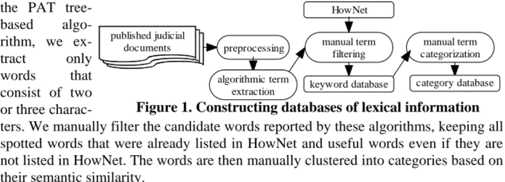
Although employing a machine-readable lexicon is essential for our work, relying completely on HowNet will not provide satisfactory results. HowNet was developed by excellent researchers in China, and it is not deniable that HowNet provides invalu-able information about Chinese words. Nevertheless, it is also true that the Chinese languages used in Taiwan and in China have become a bit different due to the separa-tion in the past half century. In addisepara-tion, HowNet may not include all legal terms that we need. For these reasons, we employ HowNet to find useful words for the legal applications, and Figure 1 shows the flow of how we acquire the lexical information.

We apply Chien’s PAT tree-based algorithm [4] and our own algorithm, TermSpotter, for spotting possible Chinese words from a training corpus. When using

the PAT tree-based algo-rithm, we ex-tract only words that consist of two or three

charac-ters. We manually filter the candidate words reported by these algorithms, keeping all spotted words that were already listed in HowNet and useful words even if they are not listed in HowNet. The words are then manually clustered into categories based on their semantic similarity.

Procedure: TermSpotter (input: a training corpus; output: a list of candidate words)

1. Scan the corpus, and obtain frequencies of all bigrams

2. Concatenate bigrams that have similar occurrence frequencies into longer words, preferring those have higher frequencies

3. Save all n-grams that exceed the threshold for occurrence frequency into a word-list

4. Remove selected words from the wordlist, and return the resulting wordlist Our method for spotting terms in our training data is actually very simple. The TermSpotter aggregates consecutive n-grams that have similar and high occurrence frequencies into a longer word. At step 2, two neighbor n-grams will be aggregated if their frequencies did not differ more than 50% of their individual frequencies. At step 3, n-grams are considered frequent if they occurred more than 30 times. The choices of 50% and 30 were arbitrary, which make TermSpotter perform satisfactorily so far. Step 4 removes words that meet specific conditions, and we subjectively set up the conditions.

We employed both TermSpotter and Chien’s algorithm to look for useful terms from 10372 real world indictment documents. The very first step in processing the legal documents that were published as HTML files was to extract the relevant sec-tions at the preprocessing step. We then ran TermSpotter and Chien’s algorithm over the corpus to get the candidate words, and manually filtered the list to obtain the keyword database. At the manual filtering step, all extracted words that were also included in HowNet would be saved in the keyword database. We subjectively de-cided whether to save the extracted words that were not included in HowNet. After checking each of the algorithmically extracted words, we found 1847 useful words that were already included in HowNet. We also found 832useful words for the legal application, but they were not included in the original HowNet. In total, we have 2679 words in the keyword database.

To enhance the information encoded by the words, we manually categorized words which have similar meanings in legal applications. For instance, we have a category for location which includesChinese words for banks, post offices, night markets, etc., and we also have a category for vehicle which includes such Chinese words as

pas-senger cars, busses, taxes, and trucks. We have 143 categories that include more than two Chinese words, and we treat a word as a single-word category if that word carries a unique meaning. In categorizing the words, we ignored the problem of ambiguous words, so a word was assumed to belong to only one category. Although making such

category database preprocessing manual term

categorization keyword database manual term filtering HowNet published judicial documents algorithmic term extraction

a strong assumption is subject to criticism, we consider it worthy of exploration be-cause words might carry specific meanings in phrases in legal documents.

4 Phrase-based kNN classification

Instance-based learning [11] is a technique that relies on past recorded experience to classify future problem instances, and kNN methods are very common among differ-ent incarnations of the concept of instance-based learning. By defining a distance measure between the past experience and the future problem instance, a system se-lects k past experiences that are most similar to the future problem instance, and clas-sifies the future instance based on the classes of the selected k past experiences.

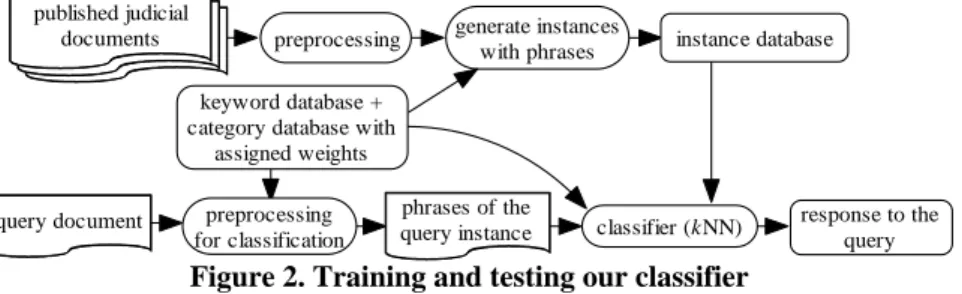
The appropriateness of the similarity measure is crucial to the success of a kNN-based system. Given a segmented Chinese text as we explained in Section 2, we can treat each past experience as a vector or a bag of Chinese words. The distance meas-ure can be defined in appropriate ways [12]. In this paper, we report our experience in using phrases as units of indexing for legal documents in Chinese, and in learning the weights for phrases in classifying documents. Figure 2 shows the flow for training and testing our classifiers, and major components are explained in this section.

4.1 Identifying phrases and learning their weights

Although it is intuitive that using phrases will lead to more precise indexing of the past documents, it is far less clear about how we choose phrases from sentences [1, 2, 3]. Moreover, it is not even clear that how we define “sentences” in Chinese. Although modern Chinese writing adopts punctuations such as commas and periods, a sequence of words ended with periods do not necessarily correspond to just one sentence as they normally do in English. It is very common that a sequence of Chi-nese words ended with a period can be translated into multiple English sentences. In this work, we choose to use commas and periods as terminators for Chinese sentences.

Given a Chinese sentence, we can segment the sequence of characters into a se-quence of words. Now, with this sese-quence of words, can we determine a phrase that actually stands for the main idea of the original sentence? It seems that this is a tough question that we cannot solve without resorting to semantic analysis of the original text. If we may solve this problem now, we might have found a solution to the prob-lem of exact indexing of documents which is an essential challenge for information retrieval. To circumvent this difficulty, we record all possible word pairs formed by

instance database generate instances

with phrases preprocessing

query document phrases of the _{classifier (kNN)}

query instance response to the_query preprocessing

for classification keyword database + category database with

assigned weights published judicial

documents

words in the sentence, and disregard those pairs which do not occur more than 10 times in the training documents. We then take the union of word pairs for all sen-tences in a preprocessed document as the feature list of the document. We employ this procedure in ovals labeled with generate instances with phrases and

preprocess-ing for classification in Figure 2.

Before we explain ways of assigning weights to phrases, we elaborate on how we define phrases in more details. Assume that, after being segmented, a sentence in-cludes three words, α, β, γ. We will preserve the original ordering of these words, and come up with three combinations, i.e., α−β, α−γ, and β−γ, as the phrases for the sen-tence. As a result, if we have a document that includes this sentence, these word pairs will all be included in the instance that represents the original document. We recog-nize that this might not be a good design decision, but doing so relieves us of the task of determining which phrase is the “most representative” of the original sentence for the current exploration.

It is expected that with appropriate weights, weighted kNN methods provide better performance than plain kNN methods [11]. Hence we would also like to assign weights to phrases. The weights for phrases should reflect their potential for helping us to correctly classify documents, so defining weights based on the concept similar to the inverse document frequency [12] is desirable. As we mentioned in Section 3, we actually have converted some words to their semantic categories. Hence, we will assign weights to phrases at the level of semantic category, rather than to the phrases at the word level.

We explore two methods for assigning weights to phrases. Let S={s1, …, si, …, sn}

be the set of different types of documents in an application. Assume that a phrase κ appears fi times in documents of type si. Let pi be the conditional probability of the

current document belonging to si, given the occurrence of κ. We may assign the

quan-tity defined in (1) as the weight of κ. Notice that the denominator in (1) assimilates the formula of entropy. Hence a phrase with larger w1 will collocate with fewer types

of documents. We also explore the applicability of (2). Qualitatively, w2 is similar to w1 in that a phrase with larger w2 will collocate with fewer types of documents.

∑ ∑ ₌ = ₌ − = n r r i i n t t t f f p where p p w 1 1 1 , log 1 ) (κ (1)

(

)

Now that we have converted the original documents into instances that are repre-sented by sets of phrases and that we have assigned weights to phrases, we are ready to define the similarity measure between instances for our classifier that adopts the

kNN approach. Assume that we have two instances i1 and i2, each representing a set

of key phrases. Let u1,2 denote the intersection of i1 and i2. We explore two methods,

shown in (3) and (4), for computing the similarity between i1 and i2. The basic

in-stances being compared. Two inin-stances are relatively more similar if they share more common phrases. Formulas (3) and (4) differ only in how we combine the two ratios.

2 ) of weights total of weights total of weights total of weights total ( ) , ( 2 1,2 1 1,2 2 1 1 i u i u i i s = + (3) ) of weights total ( ) of weights (total of weights total ) , ( 2 1 1,2 2 1 2 i i u i i s × = (4)

4.3 More design factors

In addition to how we obtain basic words, how we define weights, and how we define similarity measure between instances, there are other design decisions that we can manipulate. It is interesting to consider whether we should take into account the part of speech (POS) of the words when we construct phrases. Since our phrases consist of only two words, it is natural for us to consider only verbs and nouns in forming the phrases. Under this constraint, we could have phrases of the form verb, verb-noun, noun-verb, and noun-noun. If we interpret our phrases as basic events in the descriptions of the criminal violations, we might prefer to employ phrases led only by verbs in computing similarity between instances. Hence, we can compare the per-formance of classification when we consider any word pairs and when we consider only phrases with leading verbs.

The other design factor that we have considered is to limit the source of phrases. Recall the way we construct phrases in Section 4.1. If a sentence contains many basic words, we would create many combinations of these basic words, potentially intro-ducing noisy phrases into our databases. Though the noise thus resulted may not interfere the classification very much, it may degrade the computational efficiency of the classifier. This observation leads us to screen sentences from where we would obtain phrases. For the experiment results reported in the following section, we con-sider sentences that contain no more than 16 Chinese characters which can be seg-mented into no more than 3 words. Experimental results under other settings are in-cluded in a longer version of this paper.

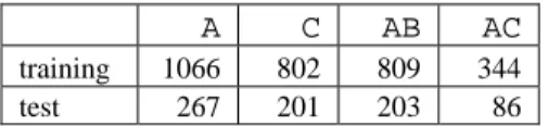
5 Experimental evaluations

We evaluated our classi-fier with real world judi-cial documents. Table 1 shows the quantities of the documents used for

the task of classifying documents based on the prosecution categories. Table 2 shows quantities of docu-ments for the task of classifying documents based on the cited

arti-Table 2. Number of cases in different combina-tions of cited articles for gambling cases

A C AB AC

training 1066 802 809 344 test 267 201 203 86

Table 1. Number of cases in different prosecution categories X1 X2 X3 X4 X5 X6

training 1600 1600 1600 1600 710 241 test 400 400 400 400 179 60

cles. We acquired the documents from the web site of the Judicial Yuan, Taiwan (www.judicial.gov.tw). We continue to use the notation for representing different types of documents, which are discussed in Section 2.

Since our work is not different from traditional research in text classification, we embraced such standard measures as precision, recall, the F measure, and accuracy for evaluation [12]. Let pi and ri be the precision and recall of an experiment, F is

defined as (2×pi×ri)/(pi+ri). Due to page limits, we must summarize the classification

quality for all different types of documents, and we took the arithmetic average of the

precision, recall, F, and accuracy of all experiments under consideration.

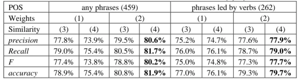
Tables 3 and 4 show statistics about the performance of our classifier. These tables employ the same format. The top row indicates whether we considered all types of word pairs or only phrases that were led by verbs, as we discussed in Section 4.3. The second row indiecates whether we employed formula (1) or (2) for defining weights of phrases, and the third row indicates whether we computed similarity between instances by formula (3) or (4). The numbers in the top row indicate the quantities of phrases that were obtained from the training documents.

Table 3 shows the statistics for the experiments for prosecution category-based classifiction, when we extracted phases from sentences which contained no more then 16 Chinese characters which were segmented into no more than three words. Using this setup, we obtained 1504 phrases when we considered all types of phrases, and, if we ignored pharses that were not led by verbs, we obtained 989 phrases from the training documents. We observed that no matter whether we consider POS of constituents of the phrases, the combination of formulas (2) and (4) would offer the best performance. This proposition held when we repeated the same experiment procedure for setups where we obtained phrases from sentences of different number of characters and words. Results for classifying cases based on cited articles, i.e., statistics in Table 4, furuther support that (2) and (4) together outperform for the task of cited article-based classification than other combinations of the formulas. Assuming that we use (1) for defining weights, (3) seems to be a better choice for

Table 3. Classification based on prosecution categories (3,16)

POS any phrases (1504) phrases led by verbs (989)

Weights (1) (2) (1) (2) Similarity (3) (4) (3) (4) (3) (4) (3) (4) precision 74.7% 81.9% 79.7% 85.7% 72.2% 77.1% 77.9% 85.5% Recall 74.3% 67.3% 79.1% 81.5% 70.3% 63.4% 76.2% 81.5% F 70.0% 68.8% 77.7% 82.1% 66.1% 63.9% 74.9% 82.2% accuracy 74.9% 73.2% 81.6% 86.2% 70.7% 69.0% 78.6% 85.4%

Table 4. Classification based on cited articles (3,16)

POS any phrases (459) phrases led by verbs (262)

Weights (1) (2) (1) (2) Similarity (3) (4) (3) (4) (3) (4) (3) (4) precision 77.8% 73.9% 79.5% 80.6% 75.2% 74.7% 77.6% 77.9% Recall 79.0% 75.4% 80.5% 81.7% 76.0% 76.1% 78.7% 79.0% F 77.4% 73.8% 78.8% 80.2% 75.0% 74.8% 77.3% 77.7% accuracy 78.9% 75.4% 80.8% 81.9% 77.0% 76.1% 79.3% 79.7%

computing similarity between instances.

Statistics, particularly those for the combination of (2) and (4), in both Tables 3 and 4 do not show any relative superiority in classification quality for whether we should consider POS of the constituents of the phrases. We do not consider the differences in the statistics significant although the averages for not considing POSs seem a bit better. However, we would have used more than 40% of number of phrases in the classification for considering all types of phrases. Using phrases that were led by verbs clearly had an edge on computational efficiency.

Corresponding numbers for the combination of (2) and (4) in Tables 3 and 4 support the intiution that classification based on prosecution categories is relateively easier than classification based on cited articles. The same observation had been reported by Liu and Liao [10]. However, we have to interpret this indication of our statistics carefully, because all cases that were used for obtaining Table 4 committed the crime of gambling in different details, while cases for obtaining Table 3 belonged to a range of different prosecution categories not including gambling, as we reported in Section 2. In addition, corresponding numbers for other columns in Tables 3 and 4 do not fully support the intuition. Cases that belong to prosecution categories in our experiments may contain related criminal violations that disoriented our classifier. For instance, it should not be surprising that one would describe something that related to larceny (X1) before one could describe how one received stolen property (X4). Therefore differentiating X1 and X4 may not be easier than telling A and AC apart for gamling cases.

6 Concluding remarks

We reported an exploration among a myriad of possible ways of applying phrases to classifying judicial documents. The preliminary results are encouraging. Compared with the results reported in [9], we are able to achieve better quality of classification when our target prosecution categories are much closer than those used in previous studies. For the task of classifying cases based on cited articles, our method provides comparable quality with those reported by Liu and Liao [10]. However, our training method is more succinct and easy to understand and implement than the introspective learning method used in [10]. Our current system employs only relative frequencies of phrases among different types of documents, but Liu and Liao had to learn and adjust weights for each keyword in each training instance. Nevertheless, our advantage may have come from that we have to manually filter the Chinese words, and Liu and Liao’s approach does not need human intervention at all. Similar to Liu’s results, our results are better than those reported by Thompson [11]. Our results are also better than those achieved by pioneers of the phrase-based approach [2, 3], partially because the legal domains employ more specific terms in the judicial documents.

Besides the inspiring results, the exploration left us more questions to study. Indeed, pioneers had reported many challenges for the phrase-based approach [2, 3]. It should be clear that coming up with an effective method for weighting the phrases is not easy. It is also difficult to determine how we obtain important phrases for