利用賽局理論之多網路系統最佳化入侵防護策略

國

立

交

通

大

學

電信工程研究所碩士班

碩

士

論

文

利用賽局理論之多網路系統最佳化入侵防護策略

Optimal Intrusion Protection Strategy for Multiple Network

Systems using Game Theory

研 究 生：李 彥 良

指導教授：李程輝 教授

利用賽局理論之多網路系統最佳化入侵防護策略

Optimal Intrusion Protection Strategy for Multiple

Network Systems using Game Theory

研 究 生：李彥良 Student：Yen-Liang Lee

指導教授：李程輝 Advisor：Tsern-Huei Lee

國 立 交 通 大 學

電信工程研究所

碩 士 論 文

Submitted to Institute of Communications Engineering College of Electrical Engineering and Computer Engineering

National Chiao Tung University in partial Fulfillment of the Requirements

for the Degree of Master

in

Computer and Information Science

July 2013

Hsinchu, Taiwan, Republic of China

I

利用賽局理論之多網路系統最佳化入侵防護策略

學生：李彥良 指導教授：李程輝

國立交通大學電信工程研究所碩士班

摘

要

II

Optimal Intrusion Protection Strategy for

Multiple Network Systems using Game

Theory

Student:

Advisor: Prof.

Institute of Communication Engineering

Electrical and Computer Engineering College

National Chiao Tung University

ABSTRACT

In this paper, we present a game-theory based strategy for protecting multiple network systems. We consider the interactions between the attacker and the defender as a two-player, and non-cooperative game in both sequential and simultaneous mode. Optimal strategies for both the attacker and the defender are derived.

III

誌

謝

能夠完成這篇論文，我必須感謝我的指導教授－李程輝教授。

他總是不辭辛勞地教導我作研究的態度，在這兩年的研究所生活

中，我不只學習到專業知識還有獨立思考的能力，更重要的是我從

老師身上學到了研究以及做事的正確態度。這些處理事情的態度對

我將來工作上會有很大的幫助。

感謝我的朋友，在我最焦慮徬徨無助時，給我建議和鼓勵，陪

我紓解壓力，讓我不致於被壓力吞沒。

最後謹將此論文獻給身邊所有愛我的人及我愛的人。

2012/07 李彥良

IV

目

錄

中文摘要

I

英文摘要

II

誌謝

III

目錄

IV

圖目錄

V

表目錄

VI

Chapter 1. Introduction

1

Chapter 2. Background and Problem Formulation

3

2.1 An Overview of Game Theory 3

2.2 Prisoner’s Dilemma 5

Chapter 3. System Model

7

Chapter 4. Analysis

9

Chapter 5. Simulation

13

Chapter 6. Conclusion

27

V

圖 目 錄

Figure 1. An overview of game theory 5

Figure 2. System model 7

Figure 3. Results of the attacker 8

Figure 4. For k=n-1, defender chooses systems with randomly determined

probabilities 14

Figure 5. For k=n-1, defender applies optimal strategy 15

Figure 6. For k=n-1, attacker chooses systems with randomly determined

probabilities 16

Figure 7. For k=n-1, attacker applies optimal strategy 17

Figure 8. For k=n+1, defender chooses systems with randomly determined

probabilities 18

Figure 9. Defender applies optimal strategy 19

Figure 10. Attacker chooses systems with randomly determined probabilities 20

Figure 11. Attacker spplies optimal strategy 21

Figure 12. Defender chooses systems with randomly determined probabilities 22

Figure 13. Defender applies optimal strategies 23

Figure 14. Attacker chooses system with randomly determined probabilities 24

VI

表 目 錄

Table 1. Payoffs of prisoner’s dilemma 6

Table 2. Parameters of the simulations 13

Table 3. Average scores when of k=n-1 25

Table 4. Average scores when of k=n+1 26

1

Chapter 1. Introduction

1.1 Introduction

Today we live in a world that is highly dependent on the Internet. Smart phones, personal computers, traffic lights, etc., all rely on the network to provide their services. With these services, our lives become much more convenient than ever. However, network suffers from security problems. Network security has become a challenging issue because many new network attacks have appeared increasingly sophisticated and caused vast loss to network resources. How to protect multiple network systems with limited resources is one of the critical issues we must face.

In this paper, we assume that there is an intruder who wants to intrude a set of systems that are guarded by a defender. The defender can only protect one of the systems while the

intruder launches his attack. We discuss how game theory can be applied to this problem. We have derived an optimal strategy for the intruder to maximize his benefits, and an optimal strategy for the defender to minimize the intruder’s benefits.

1.2 Related works

Several papers concerning about network security using game theory have been proposed.

In[1], Kong-wei Lye and Jeannette Wing model the network security problem as a general-sum stochastic game between the intruder and the defender. They also compute the Nash equilibrium strategies for the players.

In[2], Sankardas Roy, Charles Ellis, Sajjan Shiva, Dipankar Dasgupta, Vivek Shandilya, and Qishi Wu categorize game theory into many different groups, discuss the relationship

2

between network security and game theory. Our system model in this paper belongs to one of the games mentioned in this paper.

In[4], Xiannuan Liang, and Yang Xiao provide a survey and classifications of existing game theoretic approaches to network security. They show the short comings of traditional solutions to network security, and that game theoretic approachs are powerful tools for solving network security problems.

3

Chapter 2. Background and Problem

Formulation

2.1 An Overview of Game Theory

Game theory describes the multi-person decision scenario as games where each person chooses the actions that results in the best rewards for himself. Here we introduce some of the terminologies of game theory.

Game

The interaction among rational, mutually aware players, where the decisions of some players impacts the payoffs of others. A game is described by its players, each

player's strategies, and the resulting payoffs from each outcome. Additionally, in sequential games, the game stipulates the timing of moves.

Action

An action constitutes a move within a game.

Player

Any participant in a game who has more than one set of strategies and selects among the strategies based on payoffs. If a player is non-strategic, selecting strategies randomly, the player is termed a nature player.

Payoff

4

of each player. Payoffs may represent profit, quantity, or rank the desirability of outcomes. In all cases, the payoffs must reflect the motivations of the particular player.

Strategy

A strategy defines a set of moves or actions a player will follow in a game. A strategy must be complete, defining an action in every contingency, including those that may not be attainable in equilibrium. For example, a strategy for the game of checkers would define a player's move at every possible position attainable during a game.

Sequential Game

A sequential game is one in which players make decisions following a certain predefined order, and in which at least some players can observe the moves of players who preceded them.

Simultaneous Game

A simultaneous game is one in which all players make decisions without knowledge of the strategies that are being chosen by other players. Even though the decisions may be made at different points in time, the game is simultaneous because each player has no information about the decisions of others; thus, it is as if the decisions are made simultaneously.

Static Game

This is the type of game that we discuss through out this paper. Static game is a one-shot game where all players make decisions at the same time. Even though the decisions may be made at different points in time, the game is simultaneous because each player has no information about the decisions of others; thus, it is as if the decisions are made simultaneously.

5

Figure 1. An overview of game theory

In game theory, usually we have the following basic elements and assumptions:

1. Every decision player has two or more well-specified actions or sequences of actions. 2. Each possible combination of actions leads to a well-defined end-state (win, loss, or draw)

that terminates the game.

3. Each player’s end-state has its corresponding payoff.

4. All players are rational, which means that given two choices, each player would choose the one that results in higher payoff.

2.2 Prisoner’s Dilemma

We exemplify the above descriptions by introducing a well-known game: the Prisoner’s Dilemma. The prisoner's dilemma describes the story of two criminals (player I, and player II) who have been arrested for a crime being interrogated separately. They are told that if both of them keep silence, the case against them is weak and they will be convicted and punished for lesser charges. If this happens, each will be sent to jail for two years. If both of them confess, each will be sent to jail for five years. If only one player confesses and testifies against the other, the one who does not cooperate with the police would get a ten-year sentence and the one who cooperate will go free. Table 1 illustrates the structure of payoffs.

6

Table 1. Payoffs of prisoner’s dilemma

Meanings of the payoffs 0: sent to jail for 10 years 2: sent to jail for 5 years 3: sent to jail for 2 years 4: go free

In table 1, each cell of the matrix shows the payoffs for the two players. Player I’s payoff is shown as the first number in each pair, Player II’s as the second. As the upper-left cell shows, if both players confess, they get a payoff of 2 (sent to jail for 5 years). If both of them keep silence, they each gets a of 3 (sent to jail for 2 years), which is shown in the lower-right cell. If player I confesses and player II remains silent, then player I gets a payoff of 4 (going free) and player II gets a payoff of 0 (sent to jail for 10 years). This appears in the upper-right cell. The lower-left cell illustrates the reverse situation.

Nash equilibrium describes the steady state where no player, given all other players’ choice, would prefer to change his strategy because that would decrease his payoff. In the case of prisoner’s dilemma, the Nash equilibrium is reached when both players confess.

Player II

Confess Silence

Player I Confess 2, 2 4, 0

7

Chapter 3. System Model

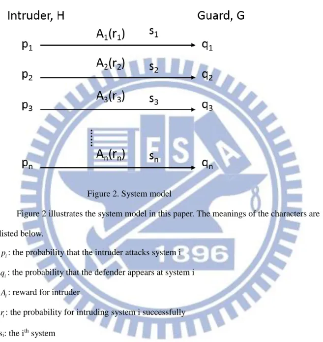
Figure 2. System model

Figure 2 illustrates the system model in this paper. The meanings of the characters are listed below.

i

p: the probability that the intruder attacks system i

i

q : the probability that the defender appears at system i

i

A: reward for intruder

i

r: the probability for intruding system i successfully si: the ith system

In this paper, we assume there is an intruder, H, who wants intrude n systems, S = {s1,

s2, …, sn}, that are guarded by a defender, G, who can only protect one system while H is

intruding. H can only intrude one system at a time. The probabilities for H to intrude systems s1, s2, …, sn are P = {p1, p2, …, pn}, respectively. The probability that H successfully enters

system i is ri. The reward for intruding these systems are A={A1, A2, …, An}, respectively,

8

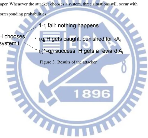
chooses to protect s1, s2, s3…, sn with probabilities Q={q1, q2, …, qn}, respectively. If H

chooses to intrude sj, and G chooses to protect sj, then H would be caught and punished for

k*Aj, where k is a constant k > 0, 1 j n. Two questions then arise, “How does the

intruder, H, decide his strategy, P, so that his expected reward can be maximized?” and “How does the defender, G, decide his strategy, Q, so that H’s expected reward can be minimized?” We will discuss the above two questions under two scenarios throughout this paper. Whenever the attacker chooses a system, three situations will occur with

corresponding probabilities.

9

Chapter 4. Analysis

The two questions, “How does the intruder, H, decide his strategy, P, so that his expected reward can be maximized?” and “How does the defender, G, decide his strategy, Q, so that H’s expected reward can be minimized?” will be analyzed in the following analyses. Analysis 1

First we consider the question about how G can minimize H’s expected reward by deciding the probabilitiy distribution of Q. In order to do this, we first list some important parameters. E[X] = 1 n i i i i p A r 



E[R] = 1 1 (1 ) n n i i i i i i i i i i p A r q k p A r q    









Assume intruder’s strategy, P, is given, our goal is to minimize E[R] by setting defender’s strategy, Q. We can have the following derivation.

1,2,..., min { [ ]} n q q q E R = 1,2,..., ₁ min { [ ] ( 1) } n n i i i i q q q i E X k p A r q   



Define V_j  p A r_{j j j}. From the above derivation, we know that G can minimize E[R] by picking up the maximum Vj, and set it to 1, no matter how H set P. This means that the

defender will always defend the system that has the maximum reward for the attacker. Next we consider how H can maximize his reward by selecting P if he knows G’s strategy.

1 2 1, 2,..., , ,..., max { min { [ ]}} n n q q q p p p E R = 1, 2,..., ₁ 1 max { ( 1) max{ }} n n i i i i i i p p p i n i p A r k p A r     



Suppose p A r_{x x x} is the maximum term, which means p A r_{x x x}  p A r_{y y y} for

,1 ,1 xy  x n  y n. We can increase 1,2,..., min { [ ]} n q q q E R by an amount of

10 1 , (A ) (1 ) n y y y x x y n y x r k A r      







this process until every p A r_{i i i} becomes the same, which means p Ar_{i i i} C for 1 i n, where C is a constant. The optimal strategy for the attacker is then derived as

1 1 1 1 i n i i j j j p A r A r   



P can be solved by using the fact that

1 1 n i i p  



We now consider the situation where H knows G’s strategy, Q. The problem to be solved is how H can maximize his reward by selecting P? The process of the maximization,

1, 2,...,max { [ ]}

p p pn E R can be derived as follows.

1, 2,..., 1, 2,..., 1 1 max { [ ]} max { ( 1) } n n i i i i i i i p p pn p p pn i i E R p A r k p A r q   







According to the above equations, we know that H can maximize his reward by setting p =1 _j

forA r_{j j}(1 ( k 1) )q_j Ar_{i i}(1 ( k 1) )q_i , 1 i n, and i j. This means that no matter what the defender’s strategy is, the intruder would always intrude the system whose expected reward, Ar_{i i}(1 ( k 1) )q_i , is the maximal.

Next, we consider how G can minimize H’s reward by selecting Q if G knows H’s strategy. Suppose there exists an optimal solution, Q*, for G, which can minimize H’s reward. We will prove that that the following statements are satisfied if G applies Q*.

I. For any two of the systems, if G guards them with a probability > 0, then their expected rewards are equal and would be

1

max{ }_i

i n V

  .

11

reward of the systems that are guarded with probability > 0.

For the convenience of analysis and reading, we define the following parameters.

(1 ( 1) )

i i i i

W Ar  k q : expected reward of system i (4.7)

F: the set of systems such that jF if and only if

1 , max{ } j f f i i n W W W W     . |F|: number of elements in F Proof of statement I:

We want to prove that if q_h* 0 , and qi*>0, then W_hW_j. This can be proved by

contradiction. Suppose that if qh* 0 , and qi*>0, then Wj Wh. Let qj'qj* , and

' *+

h h

q q  such that W_j'A r_{j j}(1 ( k 1)q_j')A r_{h h}(1 ( k 1)q_h')W '_h . In this way, we find that

1

max{ }_i

i n W

  can be further reduced, meaning that the intruder’s reward can be

reduced, which implies that Q is not an optimal solution for G to minimize H’s reward. Therefore a contradiction occurs. Statement I is proved.

Proof of statement II:

We want to prove that if qh* 0 , then WhA rh h A rj j(1 ( k 1) *)qj Wj, where

qj*>0. This can also be proved by contradiction. First we suppose that if q_h*0, then

h j

W W . Let q_h'q_h*



(1 ( 1) ')>A (1 ( 1) '),

h h h j j j

A r  k q r  k q  j F. In this way we find that

1

max{ }_i

i n W

  can be

further reduced, meaing the intruder’s reward can be reduced, which implies that Q is not an optimal solution for G to minimize H’s reward. Therefore a contradiction occurs. Statement II is proved.

After proving the above two facts, we can calculate Q* as follows.

Let V =A (1 (_{i i i}r  k 1) )q_i C i, where C is a constant (4.8) We can derive

12 1 1 1 (1 ) 1 1 i n i i j j j n k q k A r A r      

_

by using the fact that

1 =1 n i i q 



Note that in order to satisfy equation (), some of the qi may be smaller than 0, which is

undefined. This situation can be avoided by setting k n 1. Thus we have proved that Q* is the optimal solution by proving statement I and II to be true.

13

Chapter 5. Simulation

From previous discussions, we know that when k=n-1, then the expected reward of the intruder would be 1 1 ( 1) n n i i i i i i i i i p A r k p A r q    









This is a fair scenario for both the attacker and the intruder. Because no one can get reward in this game. In this paper, we present our simulation results to verify that our strategies are optimal.

Table 2. Parameters of the simulations

Number of systems 4

Number of rounds 10000

Reward for each system {23, 24, 3, 14}

Success probability of each system {50%, 50%, 50%, 50%}

Table 2 shows the parameters used in our simulation. Assume there are a total of four systems. The rewards for each of them are 23, 24, 3, and 14 respectively. Every system has a intruding success probability of 50%. We simulate the attacker’s reward in a 10000 round sequential game.

Firstly, we show the simulation results where k=n-1, and the defender chooses the intruding system first in each round of the game. In the first simulation, the defender chooses systems with randomly determined probabilities, and the attacker chooses the system that has the maximum expected reward.

14

Figure 4. For k=n-1, defender chooses systems with randomly determined probabilities In figure 4, the defender chooses systems 1, 2, 3, and 4 with probabilities 41.09%, 34.73%, 15.83%, and 8.35%. The average reward for the attacker during the 10,000 round game is 4.63. Apparently, the attacker’s strategy worksfor him, meaning that he can get a positive reward by using this strategy. Next, let us see what happens if the defender applies our optimal strategy.

15

Figure 5. For k=n-1, defender applies optimal strategy

The average reward in figure 5 is 0.17. Because the defender applies the optimal strategy, the expected rewards of all systems become the same, making the atttacker impossible to pick up the system that has the maximum expeced reward. As a result, the attacker will always get an average reward that is less than that of figure 4. This shows that our strategy for the defender is effective for the defender for reducing the attacker’s reward.

Next, we consider the scenario where the attacker makes his decision first in each round of the game. In this simulation, the attacker chooses systems with randomly determined probabilities, the defender will always choose the system that has the maximum pjAjrj term,

where 1 j n.

16

Figure 6. For k=n-1, attacker chooses systems with randomly determined probabilities In figure 6, the attacker chooses systems 1, 2, 3, and 4 with probabilities of 13.48%, 2.90%, 41.80%, and 41.82% respectively. The average reward in figure 6 is -2.84. Next, we see how the results change if the attacker applies the optimal strategy we derived in this paper.

17

Figure 7. For k=n-1, attacker applies optimal strategy

In the above figure, the average reward for the attacker is 0.01. Compare figure 7 with figure 6, we can see clearly that the average reward has increased. This is because when the attacker applies the optimal strategy, the defender has no informatin about which system the attacker may intrude.

We next show the simulation scenario where k>n-1 (here we set k=n+1). This is the case that is beneficial for the defender. Again, in the first simulation, the defender chooses systems with randomly determined probability, while the attacker chooses the system that has the maximum expected reward.

18

Figure 8. For k=n+1, defender chooses systems with randomly determined probabilities In figure 8, the defender protects systems 1, 2, 3, and 4 with probabilities 1.65%,

40.03%, 19.29%, 39.03%. The average reward in the 10,000 round game in figure 8 is 10.42. Compare figure 8 with figure 4, we can clearly see that the average score is decreased. This is because the penalty multiplier is set to a value that is beneficial for the defender. Next we see how the average score changes when the defender applies the optimal strategy we derived previously.

19

Figure 9. Defender applies optimal strategy

The average score in figure 9 is -2.54. Compare figure 9 with figure 5, we see that the average score is decreased. We next show the simulation results where k=n+1 and attacker makes decision first in each round of the game. Attacker chooses systems with randomly determined probabilites in this scenario.

20

Figure 10. Attacker chooses systems with randomly determined probabilities

The average reward in figure 10 is -9.85. Compare this result with that of figure 6, we find that the average reward is decreased. This is due to the change of value in penalty multiplier, k. Next we see what happens if the attacker uses the optimal strategy.

21

Figure 11. Attacker spplies optimal strategy

The average score in the 1000 round game in figure Figure 11. Attacker spplies optimal strategy is -1.62. Compare this result with figure 10, we find that the average score is

increased. This shows that the optimal strategy is effective for increasing the attacker’s average reward.

Next, we analyze the scenario where k=n-3. This is the scenario that is beneficial for the attacker. We first show the simulation results where the defender chooses systems with randomly determined probability and the attacker always chooses the system that has the maximum reward.

22

Figure 12. Defender chooses systems with randomly determined probabilities In figure 12, the defender guards systems 1, 2, 3, and 4 with probabilities 24.45%, 39.53%, 5.78%, and 30.24% respectively. The average score of this 1000 round game is 6.39. Compare figure 11 with figure 4, we find that the average reward is increased. This is because the penalty multiplier has decreased, making the scenario beneficial to the attacker. Next, we see what happens if the defender applies the optimal strategy.

23

Figure 13. Defender applies optimal strategies

The average reward in figure 12 is 2.16. Obviously, the average reward is decreased when comparing figure 13 with figure 12. This means that the optimal strategy is effective for the defender to protect himself.

24

Figure 14. Attacker chooses system with randomly determined probabilities In figure 14, the attacker intrudes systems with probabilities 5.73%, 37.37%, 46.17%, and 10.74% respectively. The average reward of figure 14 is -1.67. Compare the above figure with figure 6, we find that the average reward is increased from -8.48 to -4.40. This is caused by the decrease in the penalty multiplier, k.

25

Figure 15. Attacker applies optimal strategy

The average reward of figure 15 is 1.93. Compare this figure with figure 14, we can clearly see that the average reward is increased, which is beneficial for the attacker. This means that the optimal strategy is effective for the attacker.

For the convenience of reading, we list the above average rewards in the following tables.

Table 3. Average scores when of k=n-1

k=n-1 defender chooses systems with randomly determined probability defender applies optimal strategy attacker chooses systems with randomly determined probability attacker applies optimal strategy Average Score 4.63 0.17 -2.84 0.01 Theoretical Score 4.66 0 -2.91 0

26

Table 4. Average scores when of k=n+1 k=n+1 defender chooses systems with randomly determined probability defender applies optimal strategy attacker chooses systems with randomly determined probability attacker applies optimal strategy Average Score 10.42 -2.54 -9.85 -1.62 Theoretical Score 10.36 -2.04 -9.61 -2.04

Table 5. Average scores when of k=n-3 k=n-3 defender chooses systems with randomly determined probability defender applies optimal strategy attacker chooses systems with randomly determined probability attacker applies optimal strategy Average Score 6.39 2.16 -1.67 1.93 Theoretical Score 6.13 2.04 -1.67 2.04

27

Chapter 6. Conclusion

In this paper, we derived the optimal strategiesfor the attacker and the defender in both simultaneous game and sequential game. From our previous analysis, we conclude that the best strategy for the attacker is

1 1 1 1 i n i i j j j p A r A r   



and the best strategy for the defender is

1 1 1 (1 ) 1 1 i n i i j j j n k q k A r A r      

_

28

References

[1] Kong-wei Lye, and Jeannette Wing, “Game Strategies in Network Security”, In Proceedings of the 2002 IEEE Computer Security Foundations Workshop, 2002.

[2] S. Roy, C. Ellis, S. Shiva, D. Dasgupta, V. Shandilya, and Q. Wu. “A survey of game theory as applied to network security”, The 43rd Hawaii International Conference on System Sciences, 2010.

[3] An Introduction to game theory 2nd _edition,

http://www.n8fan.net/fopen/a2V5d29yZD1zdHJhdGVneSthbitpbnRyb2R1Y3Rpb24rdG8rZ 2FtZSt0aGVvcnkrMm5kK2VkaXRpb24rdG9ycmVudCZsaW5rPWh0dHAlM0ElMkYlMkZ wbGF0by5zdGFuZm9yZC5lZHUlMkZlbnRyaWVzJTJGZ2FtZS10aGVvcnklMkY=

[4] Xiannuan Liang, and Yang Xiao “Game Theory for Network Security”, IEEE

COMMUNICATIONS SURVEYS & TUTORIALS, VOL. 15, NO. 1, FIRST QUARTER 2013

[5] Game Theory.net http://www.gametheory.net/dictionary/

[6] John von Neumann, and Oskar Morgenstern. “Theory of Games and Economic Behavior”, 2007

29 102 碩 士 論 文 利 用 賽 局 理 論 之 多 網 路 系 統 最 佳 化 入 侵 防 護 策 略 交 通 大 學 電 信 工 程 研 究 所 李 彥 良