國
立
交
通
大
學
機械工程學系
碩
士
論
文
質子交換膜燃料電池中流道幾何形狀對其性能影響
之數值探討
The Numerical Study of Geometric Influence of Flow Channel
Patterns on Performance of PEMFC
研 究 生:陳長新
指導教授:陳俊勳 教授
質子交換膜燃料電池中流道幾何形狀對其性能影響之數值探討
The Numerical Study of Geometric Influence of Flow Channel
Patterns on Performance of PEMFC
研 究 生:陳長新 Student:Chang-Hsin Chen 指導教授:陳俊勳 Advisor:Chiun-Hsun Chen 國 立 交 通 大 學 機 械 工 程 學 系 碩 士 論 文 A Thesis
Submitted to Department of Mechanical Engineering College of Engineering
National Chiao Tung University in partial Fulfillment of the Requirements
for the Degree of Master Science
in
Mechanical Engineering June 2009
Hsinchu, Taiwan, Republic of China
質子交換膜燃料電池
中流道幾何形狀對其性能影響之數值探討 學生:陳長新 指導教授:陳俊勳國立交通大學機械工程研究所碩士班
摘要
本論文係以數值模擬方法來探討不同幾何形狀的蛇形流場板對質子交 換膜燃料電池的性能影響,並分析此項研究參數所得出的不同變數之分佈 變化。本模擬使用商用套裝軟體 CFD-ACE+來建構一個穩態、三維、雙相流、 多物種並包含電化學反應的數值模型。論文內容可分為三部分。第一部分 主要是分析流場、溫度場及其他電化學變數在質子交換膜燃料電池內的基 本現象。從模擬結果得知,電流密度、溫度以及水含量彼此的分佈情形呈 現緊密的正相關性。而其中存在於邊緣勒條的些許差異來自於等溫的邊界 條例。另外,這三項變數從陽極流道入口逐漸向陽極流道出口遞減,說明 其分佈情形主要受制於氫氣濃度的影響。除此之外,當操作溫度超過 348K 時,液態水的生成變得相當微弱並未在電池內產生水氾濫的情形。第二部 分主要是研究在兩個不同操作溫度(323K、353K)下不同彎道角度(45°、60°、90°、120°與 135°)的流場板對質子交換膜燃料電池的性能影響。數值計 算結果顯示,因著質傳擴散速率的提升,結合 60°與 120°的流場板可以得 到最好的性能尤其在低操作電壓下(0.4–0.6 V)。然而,不同角度的流場 板的性能差異隨著操作溫度的降低而增加,說明彎道角度對性能的影響跟 操作溫度呈負相關。另一方面,從薄膜溫度分佈圖中得知不同角度流場板 的溫度分佈是相似的,說明改變流道角度並未能降低薄膜裡的溫度變化。 第三部分接著探討不同彎道寬度的流場板在相同於第二部分的操作條件下 對質子交換膜燃料電池的性能影響。從模擬結果得知,因著物質擴散能力 的提升,擁有較寬彎道的流場板可以得到最好的性能。然而,從電流密度 及溫度的分佈圖中得知,該兩項變數在較寬彎道流場的薄膜中分佈地相當 不平均並且伴隨著熱點存在於彎道裡,而此現象對薄膜的使用壽命有相當 程度的傷害。
The Numerical Study of Geometric Influence of Flow Channel Patterns on Performance of PEMFC
Student: Chang-Hsin Chen Advisor: Prof. Chiun-Hsun Chen
Department of Mechanical Engineering National Chiao Tung University
ABSTRACT
This study numerically investigated how the geometry of serpentine flow pattern influences performance of proton exchange membrane fuel cell (PEMFC), and analyzed how these parameters lead to different distributions of model variables. Three-dimensional simulations were carried out with a steady, two-phase, multi-component and electrochemical model, using CFD-ACE+, the commercial CFD code. This thesis consists of three parts. In first part, the fundamental behaviors of the flow field, temperature and the electrochemical variables inside a PEMFC are analyzed. From the numerical results, it shows a close and positive correlation between the distributions of current density, temperature and water content with only a slight discrepancy existing at the marginal rib due to isothermal conditions. Also, these three variables decrease gradually from anodic inlet toward anodic outlet, indicating that their distributions are principally dictated by the hydrogen concentration. Additionally, with the cell temperature increased beyond 348K, liquid water
formation doesn’t appear to be considerable nor result in flooding effect inside the cell. In the second part, the effects of bend angle on the PEMFC performance is studied with various angles (45°, 60°, 90°, 120° and 135°) with cell temperature of 323K and 353K. The numerical results indicate that the combination of 60° and 120° enables flow pattern to achieve the highest performance, especially at low operating voltages, due to the increase mass diffusion rate. Also, the differences in performance for different angles become more noticeable with decreasing cell temperature, implying that the influence of bend angle on the performance is inversely proportional to the operating temperature. On the other hand, the temperature distributions of flow patterns in the membrane with different angles are more or less similar indicating the variation of temperature in the membrane is not reduced from the change of bend angles. In the third part, the effects of bend width on the PEMFC performance are subsequently studied under the same operating conditions applied in the second part. Simulation results show that flow pattern with wider bend width achieves the highest performance compared to patterns with narrower width results from the enhanced mass diffusion. However, the distributions of current density and temperature in the membrane with wider bend show a high non-uniformity with the existence of hot spot at bending areas that is fatal to membrane lifetime.
誌 謝
回首兩年在實驗室的時光,雖不算長,但卻是刻骨銘心。從一開始模型的建立、測 試到最後的收殮,有太多滾燙的淚水與無盡的感謝。能進入燃燒防火實驗室,心裡是感 恩的,其中無數的試煉與挑戰,使我得以成長,也因此使我不斷的進步。 感謝我的恩師-陳教授。因著老師的教導、賞賜與肯定,使我能在大三時開始做專 題研究,並在大四時進入實驗室學習並且申請到國科會大專生研究計畫,以及一年完成 碩士學位的表現,對此我永遠感激在心。 謝謝好朋友暨學長的瑭圓,對於在研究及課業上給予許多的幫助,並且一起分享了 生活中許多的快樂。謝謝俊翔學長在研究的事上給予了我許多的教導。謝謝育誠學長對 於課業及事業給予了我許多的教導,並且在硬體上提供了相當大的幫助,使得模擬得以 順利完成。謝謝耀文學長在課業上有許多的分享。謝謝遠達、彥成及榮貴三位學長對於 論文上的教導與幫助。謝謝義嘉從大學時所分享的友情。謝謝家維、金輝、智欽及育祈 學長們及信錡的關照。 最後的感謝歸於我的家人及親人,因著您們的關心及付出,使我渡過許多的難關, 是您們的支持,使我不畏艱難。兩年在實驗室的生活,謝謝您們所給予我的幫助,這是 耶穌基督的恩典,因著信靠使這工作得以完成。CONTENTS
摘要 ... i
ABSTRACT ... iii
誌謝 ... v
CONTENTS ... vi
List of Tables ... viii
List of Figures ... ix Nomenclature ... xiii Chapter 1 Introduction ... 1 1.1 Background ... 1 1.2 Literature Review ... 4 1.2.1 Modeling Development ... 4
1.2.2 Investigation of PEMFC Design and Operation ... 6
1.3 Scope of Present Study ... 10
Chapter 2 Simulation Model ... 15
2.1 Model Descriptions ... 15
2.2 Model Assumptions ... 17
2.3 Governing Equations ... 18
2.3.1 Continuity and Momentum Equations ... 18
2.3.2 Energy Equation ... 20
2.3.3 Species Equation ... 21
2.3.4 Electrochemical Reaction ... 23
2.3.5 Current Equation ... 24
2.3.7 Concentration Loss ... 28
2.4 Boundary Conditions ... 29
Chapter 3 Numerical Methods ... 35
3.1 Introduction to CFD-ACE+ software ... 35
3.2 Numerical Method for CFD-ACE+ ... 35
3.2.1 Finite-volume method ... 35
3.2.2 SIMPLEC scheme ... 37
3.3 Computational procedure of PEMFC simulation ... 40
Chapter 4 Results and Discussion ... 45
4.1 Fundamental Behaviors of Reference Case ... 46
4.2 Effects of Bend Angle ... 53
4.3 Effects of Bend Width ... 59
Chapter 5 Conclusions and Future Works ... 102
5.1 Conclusions ... 102
5.2 Future works ... 103
List of Tables
Table 2.1 Geometries of Model ... 16
Table 2.2 Electrochemical parameters and transport properties ... 16
Table 3.1 Grid independence test ... 41
Table 3.2 Grid for different components... 41
Table 4.1 Operating conditions of the reference case. ... 45
Table 4.2 Operating conditions ... 53
List of Figures
Fig. 1.1 Cross section of a PEMFC illustrating steps of electrochemical reaction
and major structure. ... 12
Fig. 1.2 Schematic of fuel cell I-V curve with three losses that influence the curve. ... 13
Fig. 1.3 Pictorial illustration of the effect of a leakage current loss on overall fuel cell performance. ... 14
Fig. 2.1 Flow field pattern in PEMFC (a) 45-135; (b) 60-120; (c) 90-90, respectively. ... 31
Fig. 2.2 Flow field pattern in PEMFC (a) 1007; (b) 1010; (c) 1020, respectively. ... 32
Fig. 2.3 Schematic of electrochemical reaction and the transfer current within a porous catalyst-containing conductor [33]. ... 33
Fig. 2.4 Schematic of the PEMFC mass transport model [3]. ... 34
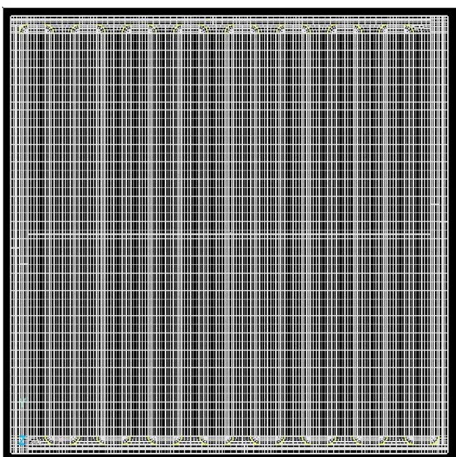
Fig. 3.1 Grid structure of current model. ... 42
Fig. 3.2 Numerical flow chart of current study [33]. ... 43
Fig. 4.1 Polarization curve of reference case. ... 64
Fig. 4.2 The specified number for each bend entrance along anodic flow channel where the corresponding values of Pe number are obtained. ... 65
Fig. 4.3 The inverse of local Peclet number at each bend entrance (0.4V). ... 66
Fig. 4.4 Distribution of current density in the membrane at 0.4V. ... 67
Fig. 4.5 Distributions of flow velocity in PEMFC at 0.4V: (a) anodic channel; (b) cathodic channel. ... 68
Fig. 4.6 Distributions of temperature: (a) at anodic channel; (b) in the membrane; (c) at cathodic channel. ... 69
Fig. 4.7 Distribution of hydrogen concentration on the interface between anodic GDL and catalyst layer at operating voltage of 0.4V. ... 70 Fig. 4.8 Distribution of oxygen concentration on the interface between cathodic GDL and catalyst layer at operating voltage of 0.4V. ... 71 Fig. 4.9 Distribution of water gas on the interface between cathodic GDL and catalyst layer and water flux in the membrane at operating voltage of 0.4V. .... 72 Fig. 4.10 Distribution of liquid water on the interface between cathodic GDL and catalyst layer at operating voltage of 0.4V. ... 73 Fig. 4.11 Distribution of water content in the membrane at 0.4V. ... 74 Fig. 4.12 Average values of temperature and water content for each current density. ... 75 Fig. 4.13 Polarization curves of flow patterns with three different bend angles at 323K and 353K. ... 76 Fig. 4.14 The inverse of Peclet number at each bend entrance ... 77 Fig. 4.15 Distributions of current density in the membrane at 323K (0.4V): (a) 45-135 flow pattern; (b) 60-120 flow pattern; (c) 90-90 flow pattern. ... 78 Fig. 4.16 Distributions of current density in the membrane at 353K (0.4V): (a) 45-135 flow pattern; (b) 60-120 flow pattern; (c) 90-90 flow pattern. ... 79 Fig. 4.17 Distributions of temperature in the membrane at 323K (0.4V): (a) 45-135 flow pattern; (b) 60-120 flow pattern; (c) 90-90 flow pattern. ... 80 Fig. 4.18 Distributions of temperature in the membrane at 353K (0.4V): (a) 45-135 flow pattern; (b) 60-120 flow pattern; (c) 90-90 flow pattern. ... 81 Fig. 4.19 Average value of temperature in the membrane at 323K and 353K. .. 82 Fig. 4.20 Distributions of water content in membrane at 323K (0.4V): (a) 45-135 flow pattern; (b) 60-120 flow pattern; (c) 90-90 flow pattern. ... 83 Fig. 4.21 Distributions of water content in membrane at 353K (0.4V): (a) 45-135
flow pattern; (b) 60-120 flow pattern; (c) 90-90 flow pattern. ... 84 Fig. 4.22 Average value of membrane water content at 323K. ... 85 Fig. 4.23 Average value of membrane water content at 353K. ... 86 Fig. 4.24 Distributions of saturation on the interface between cathodic GDL and catalyst layer at 323K. ... 87 Fig. 4.25 Distributions of saturation on the interface between cathodic GDL and catalyst layer at 353K. ... 88 Fig. 4.26 Polarization curves of flow patterns with three different bend widths at 323K and 353K. ... 89 Fig. 4.27 The inverse of Peclet number at each bend entrance... 90 Fig. 4.28 Distributions of current density in membrane at 323K (0.4V): (a) 1007 flow pattern; (b) 90-90 flow pattern; (c) 1020 flow pattern. ... 91 Fig. 4.29 Distributions of current density in membrane at 353K (0.4V): (a) 1007 flow pattern; (b) 90-90 flow pattern; (c) 1020 flow pattern. ... 92 Fig. 4.30 Distributions of temperature in membrane at 323K (0.4V): (a) 1007 flow pattern; (b) 90-90 flow pattern; (c) 1020 flow pattern. ... 93 Fig. 4.31 Distributions of temperature in membrane at 353K (0.4V): (a) 1007 flow pattern; (b) 90-90 flow pattern; (c) 1020 flow pattern. ... 94 Fig. 4.32 Average value of temperature in membrane at 323K and 353K. ... 95 Fig. 4.33 Distributions of water content in membrane at 323K (0.4V): (a) 1007 flow pattern; (b) 90-90 flow pattern; (c) 1020 flow pattern. ... 96 Fig. 4.34 Distributions of water content in membrane at 353K (0.4V): (a) 1007 flow pattern; (b) 90-90 flow pattern; (c) 1020 flow pattern. ... 97 Fig. 4.35 Average value of membrane water content at 323K. ... 98 Fig. 4.36 Average value of membrane water content at 353K. ... 99 Fig. 4.37 Distributions of saturation on the interface between cathodic GDL and
catalyst layer at 323K. ... 100 Fig. 4.38 Distributions of saturation on the interface between cathodic GDL and catalyst layer at 353K. ... 101
Nomenclature
a Water activity
ai Stoichiometric coefficient
A The y-dir. position in channel, m
B Body force, N
cref Reference molar concentration, kmol/m3
R C
c Molar concentration of hydrogen in channels, kmol/m3
R L
c Molar concentration of hydrogen in catalyst layer, kmol/m3
Cp Specific heat, J/kg K
Deff Gas effective diffusivity, m2/s
D Gas diffusivity, m2/s E Characteristic energy, K F Faraday constant, C/kmol HC Flow channel height, m
HG GDL height, m
h Mixture enthalpy, J/kg conv
C
J The mass flow rate from channels to GDL, kg/s
diff G
J The mass flow rate from GDL to catalyst layer, kg/s
i Current, A
J Mass flux, kg/m2 s
j Net current density, A/m2
j0 Reference current density, A/m2
k Boltzmann constant, eV/K keff Thermal conductivity, W/m K
p Absolute pressure, Pa q Heat flux, J/m2
R Universal gas constant, kJ/kmo K
S Surface area, m2
Sh Sherwood number
T Temperature, K
U Fluid velocity, m/s
V Volume, m3
Y Fluid mass fraction
Greek Symbols
α Mass transfer coefficient
β Kinetic constant
δ Diffusion scale length, m ε porosity ζ Relative mobility ρ Fluid density, kg/m3 η Overpotential, V κ Permeability λ Water content μ Dynamic viscosity, kg/m s σ Electrical conductivity 1/Ω m τ Shear stress tensor, N m2
τ Tortuosity
ω Production rate of water, kg/m3 s1 Φ Electrical potential, V Ω Collision integral Superscripts conv Convection diff Diffusion K Reaction kinetcs N Nerst R Molar tot Total * Dimensionless Subscripts an Anode atm Atmosphere C Flow direction ca Cathode
con Concentration losses
d Dry state
eff Effective value
F Fluid G GDL h Enthalpy in Inlet
L Catalyst layer mix Mixture
re Reversible S Solid sat Saturation
Chapter 1
Introduction
1.1 Background
Carbon dioxide generated during combustion of fossil fuels is inextricably linked to the greenhouse effect. Carbon dioxide, as other greenhouse gases, is essential to maintain the temperature of the earth. However, an excess of carbon dioxide can raise the temperature of our planet to lethal levels by absorbing and emitting infrared radiation. During the pre-industrial Holocene, the concentration of carbon dioxide was roughly 280ppm. Since then, the current concentration has grown to 384ppm, and the current global temperature has increased by 0.75°C since 1860, revealing a close bond between the growth of carbon dioxide concentration and global warming [1]. Besides, the efficiency of traditional engine is limited by Carnot cycle, according to thermodynamics. Therefore, research investigating new and clean energies has attracted considerable attention since the last decades of 20th century.
Proton exchange membrane fuel cell (PEMFC), as one of the most effective and clean technologies, may replace crude oil for generating power, and can be employed in cell phones, automobiles and power plants. The advantages of PEMFC are high efficiency, simplicity, low emissions and silence. Therefore, PEMFC, directly converting chemical energy to electricity, has received people’s attention and comprehensive study, and furthermore, it may become the dominant new power source in the future.
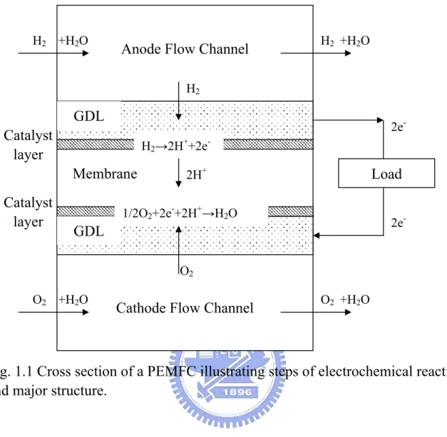
reaction happens at the anode because electrons are being liberated from hydrogen by the reaction, and electrons are being combined with oxygen at the cathode by the reduction reaction. The anode, cathode and overall reaction are:
Anode: H2(g)→Pt 2H+ +2e− (1-1) Cathode: 1/2O 2H 2e H2O Pt ) g ( 2 + + → − + (1-2) Overall: H2(g) +1/2O2(g)→Pt H2O (1-3) It should be noticed that the state of water could be either liquid or gas. The conditions that the final state of water depends on are complex, including saturation pressure, relative humidity, water content and temperature.
As shown in Fig. 1.1, the humidified hydrogen is supplied into the anode flow pattern and then it passes through the channel, meanwhile, some of the hydrogen molecules enter into gas diffusion layer (GDL). GDL made of carbon cloth provides gases an access to catalyst layer, enhances electrical conductivity and alleviates flooding effect. After that, hydrogen diffuses to anode catalyst layer, an extremely thin layer of platinum-based catalyst. Oxidation reaction happens at the anode catalyst layer, therefore, hydrogen molecules are oxidized to electrons and hydrogen ions also known as protons. Subsequently, electrons are conducted back to GDL or anode flow pattern and travel to cathode via external circuit. In the meanwhile, hydrogen ions proceed through polymer electrolyte membrane to cathode side.
As both electrons and hydrogen ions keep arriving at cathode catalyst layer, oxygen also reaches cathode catalyst layer by flowing through channel and passing through GDL. Reduction reaction happens as these three elements combine to form water, and heat is generated from this reaction. Some of the water produced from reduction reaction is drained off to flow channel and then
exits a PEMFC. Others would diffuse from cathode side to anode via the membrane. This back-diffusion phenomenon of water depends on the thickness of the electrolyte membrane and the relative humidity of each side.
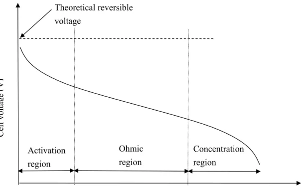
At STP, thermodynamics dictates that the reversible voltage attainable from a PEMFC is 1.23V [2, 3]. However, the output voltage of a real cell decreases as current load is applying. The decrease based on three imperative losses provides a characteristic shape in the fuel cell current–voltage (I–V) curve for a PEMFC. The three losses are:
1 Activation losses. A proportion of voltage generated is lost in driving the chemical reaction that transfers the electrons to or from electrode.
2 Ohmic losses. This voltage drop is the straightforward resistance to the flow of electrons through the material of the electrodes and the various interactions, as well as the resistance to the flow of ions through electrolyte. 3 Concentration losses. These results from the change in concentration of the
reactants at the reaction surfaces as gases are supplied. Accordingly, voltage drops due to the insufficiency of concentration.
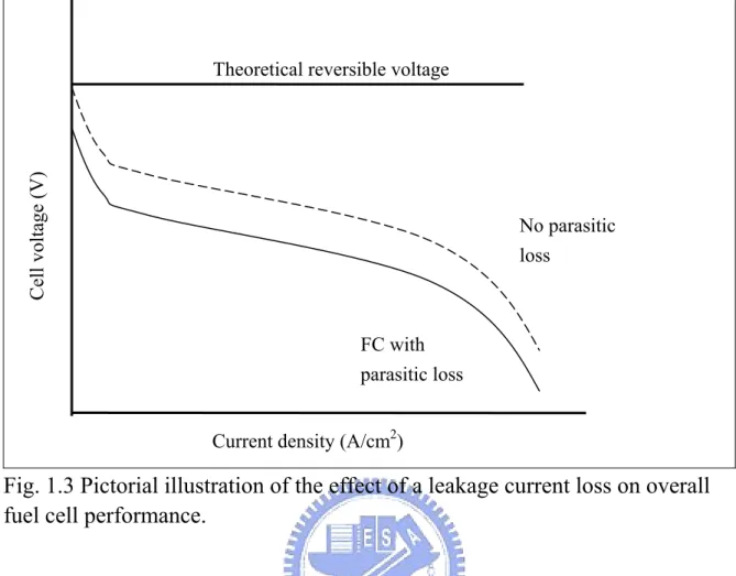
The three losses each dominates at different parts of I–V curve are shown in Fig. 1.2. The activation losses mostly affect the initial part of the curve; the ohmic losses are most apparent in the middle section of the curve, and the concentration losses are dominant in the tale of the I–V curve. Additionally, there exists an additional term associated with the parasitical loss due to current leakage and gas crossover which has a significant impact on the reversible voltage and is the reason why the actual reversible voltage is lower compared with theoretical value. Pictorially, this loss is illustrated in Fig. 1.3.
1.2 Literature Review
1.2.1 Modeling Development
Because of the high cost of PEMFC manufacturing, modeling and simulation has been developed extensively in research across the world to acquire better understanding of the fundamental processes. With deeper insight for the processes, the design cycle can be shortened substantially and the performance can be improved.
Bernardi and Verbrugge [4] proposed a one-dimensional, half-cell mathematical model for a single cell. The transport of charge and species were based on Nerst-Plank equation. And the motion of liquid water was modified by Schlogl’s velocity equation, the current transfer between membrane and solid conductor of catalyst layer were dominated by Butler-Volmer equation and the diffusivity of multi-species gas mixture was based on Stefan-Maxwell equations. Springer et al. [5] proposed an isothermal, one-dimensional, steady model for a full cell with 117 Nafion membranes. It showed that an increase in membrane resistance with increased current density and demonstrates the great advantage of a thinner membrane in alleviating this resistance problem. After a year, Bernardi and Verbrugge [6] developed the original half-cell model into a full-cell one. To get deeper insight for the gas concentration distribution and current transfer in PEMFC, a two-dimensional model was developed subsequently. Wang and Cheng’s team [7] proposed a two-dimensional model for the transport of multi-phase and multi-component gases mixture in porous medium. The results revealed that the uneven oxygen concentration profile can cause the uneven distribution of current on the chemical reaction surfaces, and the decrease of current density is due to the formation of liquid water that
decreases the oxygen concentration near the reaction surfaces. The threshold current density for single-phase and two-phase models can be obtained from this model, therefore to investigate the water transport phenomenon and the gas distribution on the cathode side. He et al. [8] proposed a PEMFC model which was two-dimensional and steady. The thermal diffusivity and evaporation speed were assumed to be constant, and therefore, the phase-change speed was limited during the reaction. The results revealed that the transport of liquid water in the porous electrodes is dominated by the shear stress and capillarity which are generated from gas and liquid water motion. In the two-dimensional model proposed by Um et al. [9] where the presence of hydrogen dilution is considered, ohmic losses is neglected in GDL and catalyst layer, hence, electronic phase is uniform across them. And oxygen is assumed to dissolve in electrolyte in catalyst layer and membrane regions. The results revealed that hydrogen was depleted at the reaction surface, resulting in substantial anode mass transport polarization, and hence, a lower current density that is limited by hydrogen transport from fuel stream to reaction site. Wang et al. [10] studied the transport phenomena of air in the cathode with two-phase model. The model was able to handle the situation where a single-phase region co-exists with a two-phase zone in the air cathode. And the results showed that capillary action is the dominant mechanism for water transport inside the two-phase zone of the hydrophilic structure. Mazumder and Cole [11, 12] proposed an accurately three-dimensional, mathematical model. This full-cell model was included in the package CFD-ACE+ produced by ESI-CFD. The model was mainly based on the multi-phase gas model from Wang et al. [7] and He et al. [8]. Thus, this model can simulate the two-phase phenomenon and the transportation of liquid water in the porous media. Also, it was constructed energy equation to solve
the problem of temperature field. Results were compared against experimental data under various operating conditions, and showed that three-dimensional modeling is the key to predicting performance of PEMFC at high current densities instead of two-dimensional one. And it also revealed that inclusion of liquid water transport greatly enhances the predictive capability of the model and is necessary to match experimental data at high current densities.
1.2.2 Investigation of PEMFC Design and Operation
PEMFC performance is strongly dominated by operating temperature, inlet relative humidity (RH) and flow pattern etc. Proper operating temperature leads to high reaction rate and low activation and ohmic losses. Appropriate RH prevents water clogging effect, moisturizes the membrane and increase the electrical conductivity of membrane. Besides, the performance of PEMFC is also depended on the distributions of reactant species, and therefore, the primary goal of flow pattern design is to increase reactant species uniformity, which can lead to uniform distributions of current density and temperature. Thus, performance would be improved, the lifetime of PEMFC would be extended, and the water flooding effect would be alleviated.
Hontañón et al. [13] tested various widths of flow channels and ribs to determine the effect of reactant species’ consumption. According to this study, optimal rib width is 1mm, and optimal channel widths are 3 and 4 mm, instead of not 1 mm. In addition, the optimal consumption rate is 45.7%. Scholta et al. [14] investigated the mass transport and electrical conductivity of a flow pattern by varying the width of channels and ribs. Their analytical results showed that an optimum value of 0.7-1 mm applies to channel and rib widths. For wide dimensions of width, the influence on mass transport or lateral electrical conductivity is significant. For very small dimensions of widths, the
manufacturing effort becomes excessively high and the probability of channel clogging via the formation of water droplets increases. The influence of aspect ratio (AR) channel height to width—was tested by Chiang and Chu [15]. According to their simulation results, membrane electrical conductivity increases when AR decreases. Shimpalee and Van Zee [16] investigated how serpentine flow fields with different channel/rib cross-sectional areas affect performance and species distributions for both automotive and stationary conditions. Their simulation results revealed that for a stationary condition, a narrow channel with wide rib spacing improves performance; however, the opposite occurs when the automotive condition is applied.
In order to study the effect of humidity on the performance, Fell et al. [17] assessed the performance of experimental flow-field designs under different levels of humidity by utilizing a single-phase isothermal model of PEMFC segments. Shimpalee [18] studied the humidification effect numerically and experimentally. The results indicated that dry steams on either anode or cathode cause a low membrane electrical conductivity and performance. On the other hand, super-saturation streams results in a higher current density such that improves the performance. A few years later, Matamoros and Brüggemann [19] adopted steady and three-dimensional models to investigate the influence of geometrical parameters on the performance under different hydrating conditions. According to their results, anode and cathode liquid water saturation affects species transport and the polymer electrolyte water content. Thus, one must simultaneously calculate both water absorption and desorption through the polymer electrolyte and liquid water saturation in anode and cathode porous media to acquire an actual view of ohmic and concentration losses in PEMFC performance. The performance of PEMFC is considerably improved by
applying 100% RH at inlet flow in comparison with 50% RH, and such better performance is achieved especially at high current densities. Zhang et al. [20] studied the effect of RH on the performance as well. The fuel cells were performed at a typical high temperature 120°C, ambient pressure and various RHs from 25% to 100%. The experimental results indicated that the membrane resistance at 25% RH is about five times higher than that at 100%. At high RHs, the membrane adsorbs more water than at low RHs which enable more ionic clusters are filled with water, and therefore, protons can transport easily as free ions through membrane, results in low membrane resistance. As expected, the PEMFC performance increases dramatically with increasing RH.
Since temperature plays an important role in PEMFC operation, the investigations for the effect of temperature on PEMFC is necessary. Coppo et al. [21] proposed a three-dimensional model that accounts for water transport in the liquid, gas and dissolved phases to study the effect of temperature-dependent parameter variations on cell performance. The results showed that in the activation regime of the polarization curve, the performance of PEMFC is mainly improved by high temperature that leads to high values of both exchange current density and charge transfer coefficient. In ohmic region of the polarization curve, benefits of running the cell at high temperature can be explained with the high membrane ionic conductivity and an increase of water diffusivity as well as water content, which results in a decrease of electrical resistance to ion transport. Al-Baghdadi [22] numerically investigated the effect of temperature distribution on material deformation. According to the results, the non-uniform distribution of stresses, caused by the temperature gradient and moisture change in the cell, induces localized bending stresses and deformation, which can contribute to delaminating between membrane, GDL
and bipolar plates, especially in the cathode side. Also, the results indicated that the maximum von Mises stress exists on the corner of flow channels and the interface between membrane and GDL.
The effects of the permeability of the electrodes and the type of gas flow distributors on the PEMFC performance were investigated by Soler et al. [23]. The results of simulation showed that the effect of permeability is not notable in the case of grooved plates, but it is rather significant in case of the solid plates. The results also revealed that the performance with solid plates declines when the permeability of the electrodes decreases. Oosthuizen et al. [24] numerically tested the effect of channel-to-channel gas crossover on the pressure and temperature distribution. The results revealed that flow crossover is only significant when the porosity of the GDL exceeds approximately 0.65. And flow crossover tends to decrease the pressure drop across the flow channel. Also, the dominant factor in determining the temperature is the thermal conductivity of the flow plate material instead of the crossover. Shimpalee et al. [25] investigated various channel path lengths to estimate the impact of flow path length on temperature distributions, current density distributions and the performance. According to their results, local temperature, water content and current density distributions become more uniform under serpentine flow-field designs with shorter path lengths or greater number of channels. Karvonen et al. [26] proposed a parallel flow pattern that had uniform flow distribution by both numerical and experimental analyses. The inlet distributor of flow pattern is narrowed that leads to a better equality of flow velocities in different channels. The difference between the largest and the smallest velocities is decreased from 16% to 8%. Sun et al. [27] presented a model considering a serpentine flow channel with trapezoidal cross-section shape. The obtained results indicated
that an increase in the trapezoidal cross-section shape ratio R is associated with an increase in the flow-cross through GDL. And R has a significant effect on the pressure variation in the flow field. As R value increases, the pressure drop increases slightly for the cross-over case. Also, an increase in Re is associated with a slight increase in the flow cross-over. Park and Li [28] numerically and experimentally studied the characteristics and effect of cross flow through the porous electrode structure between two adjacent flow channels. The results indicated that the thickness and permeability of the GDL are the two most important parameters influencing the cross flow and the resultant pressure drop. Another numerical investigation on the influence of flow pattern geometry was carried out by Jeon et al. [29] for four 10 cm2 serpentine flow-fields with single channel, double channel, cyclic-single channel and symmetric-single channel patterns at 100% and 64% inlet HR. According to their results, the double channel flow-field was found to have the highest performance at 100% inlet HR and to have most uniform current density distribution. However, for 64% inlet HR, there were little difference on performance and current density uniformity among the four serpentine flow-field patterns.
1.3 Scope of Present Study
According to the results of reference [16], low current density is observed at the bending area of flow channels, where low water content and high temperature are presented. The non-uniform distribution of water and temperature will seriously cause mechanical damage to the membrane and shorten its lifetime. Therefore, the flow pattern design in this research will focus on the improvement of cell performance and the increase of distribution
uniformity of current density, temperature and water content.
This research applies a commercial package software, CFD-ACE+, for the full-cell simulation. The investigation mainly concerns on the improvement of flow-field design by changing the bend angles and widths in flow channels. Simulations are performed in a steady, two-phase and three-dimensional model with different flow channel patterns at different operating temperatures.
This numerical investigation consists of two parts. The first one is to study the effects of bend angle on PEMFC performance with three different flow patterns at two different operating temperatures, 323K and 353K. Comparisons will be given afterward to discuss how the performance and variables distributions change with bend angle. Another part of the investigation is to study the influences of bend width under the same operation conditions as the first part. The performance and variable distributions will be compared and analyzed as well. Finally, the advantages of those configurations will be discussed.
Fig. 1.1 Cross section of a PEMFC illustrating steps of electrochemical reaction and major structure.
O2
O2
Anode Flow Channel H2
Membrane
Cathode Flow Channel
H2→2H++2e -1/2O2+2e-+2H+→H2O GDL O2 H2 H2 GDL Catalyst layer Catalyst layer Load 2e -2e -2H+ +H2O +H2O +H2O +H2O
Fig. 1.2 Schematic of fuel cell I-V curve with three losses that influence the curve.
Current density (A/cm2) Activation region Ohmic region Concentration region Cell volta ge (V ) Theoretical reversible voltage
Fig. 1.3 Pictorial illustration of the effect of a leakage current loss on overall fuel cell performance.
No parasitic loss
FC with parasitic loss Theoretical reversible voltage
Current density (A/cm2)
Chapter 2
Simulation Model
The convenience of computational fluid dynamic (CFD) provides a low-cost way to study PEMFC and enables researchers to precisely understand the flow and temperature fields inside PEMFC. Besides, the distribution of chemical parameters can be studied and the effect of each parameter can also be further compared. Based on the governing equations that describe the correlations of various properties can be developed and solved by numerical methods, providing the necessary information for PEMFC design.
2.1 Model Descriptions
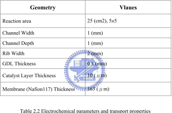
Figure 2.1 shows the three different serpentine flow patterns under investigation of bend angle (a) 45–135, (b) 60–120 and (c) 90–90, respectively. The first number in each pattern represents the first angle of the channels, and the second number represents the second angle. These two are combined to generate a complete u-turn flow channel. In addition, the patterns for investigation on the effect of bend width are shown in figure 2.2. Patterns (a) 1007, (b) 90–90 and (c) 1020, are considered. The first two numbers, 10’s, represent the channel width of 1 mm, and the last two numbers, 07 and 20, represent the bend width of 0.7 mm and 2.0 mm, respectively. 90–90 is the most conventional flow pattern applied in most researches and is considered as a reference for comparison in this study. According to the results from Scholta et al. [14], the channel and rib dimension ratio of this model is 0.5 which would lead to superior performance. Based on the results from Chiang and Chu [15],
the AR is chosen to be 1 which provides the most uniform membrane conductivity. Table 2.1 shows the detailed geometries of current model. The electrochemical parameters and transport properties from Springer et al. [5] and Mazumder and Cole [11, 12] are listed in Table 2.2.
Table 2.1 Geometries of Model
Geometry Vlaues
Reaction area 25 (cm2), 5×5 Channel Width 1 (mm) Channel Depth 1 (mm) Rib Width 2 (mm) GDL Thickness 0.3 (mm)Catalyst Layer Thickness 10 (μm)
Membrane (Nafion117) Thickness 163 (μm)
Table 2.2 Electrochemical parameters and transport properties
Parameter Values Electrochemical parameters
Transfer coefficients at anode 0.5 Transfer coefficients at cathode 1.5
Concentration dependence of H2 0.5
Concentration dependence of O2 1
GDL and catalyst layer
GDL and catalyst layer permeability 1.76×10⁻¹¹
Tortuosity 1.5 Electrode conductivity of catalyst
layer 53 (1/ohm m)
Effective surface to volume ration of
catalyst layers 1000
Membrane
Membrane porosity 0.28
Membrane permeability 1.8×10⁻¹⁸
Tortuosity 5 Electrode conductivity of membrane 1×10-20 (1/ohm m)
Bipolar Plates
Electrical conductivity Temperature dependence Reference Temperature 293 (K)
Electrical conductivity at reference
Temperature 3.5×10
-18 (ohm m)
Temperature coefficient at reference
Temperature 5×10
-4
2.2 Model Assumptions
The following assumptions are utilized to simplify simulation conditions. 1. All fluids are treated as continuums.
2. Gases are ideal gases throughout the entire model.
3. The velocity and temperature of reactant species are distributed uniformly over the channel inlet.
4. The flows are incompressible and laminar due to small Reynolds number. 5. The gas diffusion layer (GDL), catalyst layers and membrane are all
isotropic porous media with pores uniformly distributed. 6. Gravity is neglected.
7. No fuel crossover.
8. Evaporation and condensation of water is neglected. 9. Dissolution of gases in the liquid is neglected.
10. The phenomenon of double charge layer is not considered.
2.3 Governing Equations
The steady, two-phase and three-dimensional model is basically modified from the one proposed by Mazumder and Cole [11, 12]. The flow pattern has been developed from a single channel to a full-size serpentine channel with 25cm2 reaction area. The membrane domain is built for Nafion 117, and the data is available from Springer et al. [5].
The PEMFC model consists of five volume-averaged conservation equations, which are mass, momentum, energy, species and electric current conservation equations. All the equations are applied in every domain of the model. In addition, fluxes across any two different domains are automatically continuous.
2.3.1 Continuity and Momentum Equations
The continuity equation and momentum conservation equations are as follows
(
)
(
U
)
0
t
ε
effρ
+
∇
⋅
ε
effρ
=
∂
∂
(2-1)(
)
(
)
( )
κ μ ε + ε + τ ε ⋅ ∇ + ∇ ε − = ρ ε ⋅ ∇ + ρ ε ∂ ∂ U B p UU U t 2 eff eff eff eff eff eff (2-2)where ρ is the fluid density, U is the fluid velocity, p is the pressure, τ is the shear stress tensor, B is the body force, μ is the dynamic viscosity of the fluid, εeff is the effective porosity of the medium, and represents the ratio of the
volume occupied by the pores to the total volume of porous medium while the permeability κ, is the square of the effective volume to surface area ratio of porous medium. The last term in Eq. (2-2) represents Darcy’s drag force imposed by pore walls on the fluid, and leads to a significant pressure drop across the porous medium. In a purely fluid region, εeff→1 and κ→∞, and the
standard Navier-Stokes equation is recovered.
For high accuracy, mix kinetic theory is chosen to estimate the viscosity value of mixture in this research, and is expressed as
ij j j i i N 1 i mix
x
x
Φ
Σ
μ
Σ
=
μ
= (2-3)where xi and xj are the mass fraction of species i and j, μi is the dynamic
viscosity of species i and Φij is the dimensionless quantity. The dynamic
viscosity data input form [29] is linearly interpolated for each species. And the dimensionless quantity is given by
2 i j 2 / 1 j i 2 / 1 j i ij M M 1 M M 1 8 1 ⎥ ⎥ ⎦ ⎤ ⎢ ⎢ ⎣ ⎡ ⎟⎟ ⎠ ⎞ ⎜⎜ ⎝ ⎛ ⎟ ⎟ ⎠ ⎞ ⎜ ⎜ ⎝ ⎛ μ μ + ⎟ ⎟ ⎠ ⎞ ⎜ ⎜ ⎝ ⎛ + = Φ − (2-4)
where Mi is the molecular weight of species i, T is the temperature in Kelvin, σi
is the characteristic diameter of the molecular in Angstroms and Ωμ is the
) T 43787 . 2 exp( 16178 . 2 ) T 77320 . 0 exp( 52487 . 0 T 16145 . 1 14874 . 0 ∗ ∗ ∗ μ = + + Ω (2-5)
where T* is the dimensionless temperature and is defined as
Ε =
∗ kT
T (2-6)
where k is the Boltzmann’s constant and E is the characteristic energy. The details are given by Incropera [30], Wilke [31] and Hirschfelder et al. [32].
2.3.2 Energy Equation
The temperature field of each domain can be obtained from solving the energy conservation equation. The energy conservation equation can be written as
[
]
h eff T eff eff eff eff s s eff S j j V S j dt dp U q ) Uh ( h h ) 1 ( t & + σ ⋅ + η ⎟ ⎠ ⎞ ⎜ ⎝ ⎛ − ε + ∇ ⋅ τ ε + ⋅ ∇ = ρ ε ⋅ ∇ + ρ ε + ρ ε − ∂ ∂ (2-7)where h and hs are the gas mixture enthalpy and solid phase enthalpy,
respectively. ρs is the solid phase density, jT is the transfer current density which
will be discussed further in the section below, (S/V)eff is a direct representation
of catalyst loading, η is the overpotential between solid phase and electrolyte phase of the electrode, and S‧h is the enthalpy source due to phase change. The
heat flux, q, is comprised of contributions due to thermal conduction and species diffusion without considering radiation effect, and is written as
i i N 1 i
J
h
T
q
G =Σ
+
∇
λ
=
(2-8)where NG is the total number of gas phase species in the system, hi are their
and Ji is the diffusion flux of species i. The thermal conductivity, keff, of the
porous medium is an effective thermal conductivity of the pores and solid combined region and is expressed as
S eff F S eff S eff 3k ε 1 k 2k ε 1 2k k − + + + − = (2-9)
where kS and kF are the thermal conductivities of the solid and fluid regions,
respectively. The second term of on the right hand side (RHS) of Eq. (2-7) is the effect of viscous dissipation, the third term on the RHS is the work done by pressure, the last three terms in Eq. (2-7) represent electrical work, Joule heating and energy interactions due to phase change. The irreversible losses due to reaction (conversion of chemical energy to heat) manifest through the last term on the right hand side of Eq. (2-8) because the definition of enthalpy includes both the enthalpy of formation as well as sensitive enthalpy. Mix kinetic theory is also chosen for calculating the thermal conductivity across the whole domain. The data for evaluating the thermal conductivity is available from [33]. Mix Jannaf method is applied for calculating the specific heat and estimated as form: 4 4 3 3 2 2 1 0 P a a T a T a T a T R C + + + = (2-10)
where R is the value that the universal constant divided by each species’ molecular weight, and a0, a1, a2, a3 and a4 are constant vary with species kind.
2.3.3 Species Equation
The species conservation equation is estimated as form:
(
eff i)
i i i eff Y) UY J ( t ε ρ +∇⋅ ε ρ =∇⋅ +ω ∂ ∂ & (2-11)where Yi are the mass fraction of i-th species, Ji are the mass diffusion flux of
species i and ω‧i are the mass production/destruction rates of i-th species in the
gas phase. The species mass diffusion rate is expressed as
j j j i j j j i i i i i i D Y M M Y Y D Y M D M Y Y D J =ρ ∇ + ρ ∇ −ρ Σ ∇ −ρ Δ Σ (2-12)
the first term represents Fickian diffusion due to concentration gradients, and the other three terms are correction terms necessary to satisfy the Stefan-Maxwell equations for multicomponent species study. In this case, Di are the effective
diffusion coefficient of species i within porous medium, and depend on the porosity and tortuosity, τ, of the medium
Deff=εeffτD (2-13)
where the value of tortuosity is usually 1.5 in Eq. (2-13), resulting in the so-called Bruggeman model [11].
The volumetric production/destruction rate of a species i, ω‧i, due to
heterogeneous surface reaction is treated by performing a diffusion flux at the interface of the GDL and catalysts, and is obtained from the surface flux in discrete form expressed as
eff i, P i i i
V
S
Y
Y
D
⎟
⎠
⎞
⎜
⎝
⎛
δ
−
ρ
=
ω&
(2-14)where Yi denotes the mass fraction at the interface of GDL and catalyst
layer, while YPi denotes the species mass fraction in the catalyst layer and δ is
the diffusion length scale. Usually, the diffusion length scale cannot be obtained from grid in the case of porous media, because the region under consideration is already much smaller than the size of a control volume. Typically, the diffusion length scale varies locally from primary pores to secondary pores. With the consideration of continuum mechanism, Knudsen
effect is neglected in tiny pore region, and the diffusion length scale is assumed to be equal to the average pore size in this case.
However, in the case of electrochemical reactions, the volumetric production/destruction rate of a given species is expressed as
F j ) a a ( R T i P i i = − ω& (2-15) where P i a and R i
a are the stoichiometric coefficients of the products and reactants, respectively. F is the Faraday constant. Therefore, reaction-diffusion balance is necessarily required to be written as
F j ) a a ( V S Y Y D R T i P i eff i, P i i ⎟ = − ⎠ ⎞ ⎜ ⎝ ⎛ δ − ρ (2-16)
Eq. (2-16) clearly states that the reactants/products flowing through the interface where chemical reaction takes place by diffusion is equal to the volumetric production/destruction rate of a specific species from chemical reaction.
Maxwell-Stefan Model is applied for multi-species diffusion when over and above three species are involved in a diffusion process. At low density, multi-component gas diffusion can be approximated by the Maxwell-Stefan equation:
∑
≠ − = NG i j ij i j j i i pD J x J x RT dz dx (2-17) 2.3.4 Electrochemical ReactionAt the electrode catalyst layers, current is supplied from electrochemical reactions that reactant species participate at anode and cathode. Hydrogen is oxidized at the anode and oxygen is reduced at the cathode. These two reactions are driven by the potential difference between the solid phase and electrolyte phase, called the activation overpotential. The Bulter-Volmer
equation describes this phenomenon and is expressed as
[
]
[ ]
k,j j , k k N 1 k j , c j , a ref , k N 1 k j , 0 j , T )] RT F exp( ) RT F [exp( j j α = α = Λ Π × η α − − η α Λ Π = (2-18)where αa,j and αc,j are kinetic constants determined from experimentally
generated Tafel plots, αk,j are the concentration exponents of the k-th species for
the j-th step. [Λk] represents the average interfacial molar concentration of the
k-th species, and the subscript ref refers to concentration values at the reference state at which the reference current density is prescribed. The electrode potential, η, is the potential difference between the solid phase (ΦS) and the
ionic phase (ΦF) of the electrode.
The term j0,j in Eq. (2-18) is the reference current density with units of A/m3.
As a matter of fact, the reference current density at the cathode is several orders of magnitude smaller than the value at the anode. Both the reference current densities at anode and cathode are expressed as [34]
Anode: j0=1×10⁹ (2-19)
Cathode: j0=3×10⁵ exp[0.014189(T-353)] (2-20)
2.3.5 Current Equation
The continuity equation of current in any material leads to: 0
i = ⋅
∇ (2-21)
where i is the current density vector. When the material is a porous electrode, the current density is split into two parts: one flowing though the polymer electrolyte (ionic phase) denoted as iF and the other flowing through the solid
parts (electronic phase) of the porous matrix denoted as iS. Fig. 2.3 simply
shows the transfer of current within porous media. Eq. (2-18) can be written as 0
i iF +∇⋅ S = ⋅
During the electrochemical reactions, electrons are either transferred from ionic phase to solid phase or vice versa shown in figure 2.3. Thus, Eq. (2-19) can be rewritten as eff T S F V S j i i ⎟ ⎠ ⎞ ⎜ ⎝ ⎛ = ⋅ ∇ = ⋅ ∇ − (2-23)
It is generally assumed that each phase has its own electrical potential. In the ionic phase, the electrical current is denoted as electrolytic term while the current is denoted as electronic term in solid phase. Chemical reaction can only occur at the interface of electrolyte and solid when there’s interaction between these two current components. Under this assumption, application of ohm’s law to Eq. (2-23) yields
eff T S S F F V S j ) ( ) ( ⎟ ⎠ ⎞ ⎜ ⎝ ⎛ = Φ ∇ σ ⋅ −∇ = Φ ∇ σ ⋅ ∇ (2-24)
where ΦS and ΦF are the electrical potentials of the ionic and solid phases,
respectively.
2.3.6 Liquid Water Transport
The foundation of this two-phase model is an additional governing equation for the transport and formation of liquid water, given by
l g l s 1 d F l 1 d l d m g ) ( ) 1 ( ) D ( i F M ) U ( ) s ( t & + ⎟⎟ ⎠ ⎞ ⎜⎜ ⎝ ⎛ ν ρ ρ κ ς − ς ⋅ ∇ − ∇ ρ ε ⋅ ∇ = ⎟ ⎠ ⎞ ⎜ ⎝ ⎛ α ⋅ ∇ + ς ρ ε ⋅ ∇ + ρ ε ∂ ∂ − λ (2-25)
where s is the saturation of liquid water, and is defined as the ratio of liquid volume to the volume of pores. ρl is the density of liquid water and ζ is the
relative mobility of liquid water. εd is the dry porosity which represents the
is considered, pores in porous media are occupied by liquid, and the value of effective porosity decreases as the amount of liquid water in the medium increases. Therefore, εeff has the form
) s 1 ( d eff =ε − ε (2-26)
The first term in Eq. (2-25) represents the storage of liquid water in a certain domain. And the second term represents transport of liquid water by pressure-driven advection.
Membrane water content, λ, is given as the ratio of the number of water molecules to the number of charge (SO−H+
3 ) sites. It shows how intense the
electrochemical reaction is, and dictates the electrical conductivity of membrane. The value of membrane water content is determined by the activity of water vapor at the catalyst/membrane interface. The activity in the water phase, a, is xwP/Psat. xw is the mole fraction of water vapor and the saturation pressure of
water is denoted by Psat in units of atm, which can be computed from the
curve-fitted expressions provided by Springer et al. [5]
3 7 2 5 sat 10P 2.1794 0.02953T 9.1837 10 T 1.4454 10 T log =− + − ⋅ − + ⋅ − (2-27)
Membrane water content is function of water activity for the Nafion 117 membrane by weighing membranes equilibrated above aqueous solutions of various lithium chloride concentrations, and the experimental relationship of water content versus water activity, a, used in this model is
⎪ ⎩ ⎪ ⎨ ⎧ < ≤ < − + ≤ < + − + = λ a 3 8 . 16 3 a 1 ) 1 a ( 4 . 1 14 1 a 0 a 0 . 36 a 85 . 39 a 18 . 17 043 . 0 2 3 (2-28)
Eq. (2-28) is employed to calculate the value of λ based on solution of water vapor outside the membrane domain.
When water profile in the membrane has been determined, the membrane electrical resistance and the potential drop across it can easily be obtained. The electrical conductivity of Nafion 117 was proposed by Springer et al. [5], and is given by ] T 273 1 303 1 1268 exp[ ) T ( 1 00326 . 0 005193 . 0 K 303 K 303 ⎟ ⎠ ⎞ ⎜ ⎝ ⎛ + − σ = σ > λ − λ = σ (2-29)
Once the value of water content drops less than one, the membrane conductivity is assumed to be constant.
In a PEMFC, electro-osmotic water drag moves liquid water from anode to cathode. As this water built up at cathode, back diffusion occurs, resulting in the transport of water from cathode back to anode. This phenomenon is strongly dominated by capillary diffusivity. Capillary diffusivity depends on factors like the contact angle and saturation, and can be written in terms of the capillary pressure head as
ds dp D c l l μ κ − = λ (2-30)
where pc is the capillary pressure head, κl is the permeability of the liquid and μl
is the dynamic viscosity of the liquid. Based on the correlation that Springer et al. [5] proposed, capillary diffusivity is function of water content and temperature, and is expressed as [5]
⎪ ⎩ ⎪ ⎨ ⎧ − λ + ≤ λ − λ + ≤ λ λ = λ otherwise 15 / ) 26 ( 4 75 . 3 6 4 / ) 2 ( 25 . 3 5 . 0 2 4 / D' (2-31) ' 2 2 10 D ) a 108 a 7 . 79 81 . 17 ( a ) s 1 ( 10 ) K 303 ( D λ − λ + λ − + λ = (2-32)
] T 1 303 1 2416 exp[ ) K 303 ( D D ⎟ ⎠ ⎞ ⎜ ⎝ ⎛ − = λ λ (2-33)
In Eq. (2-32), s is considered as a constant with value of 0.0126.
2.3.7 Concentration Loss
During the electrochemical reaction, performance drops when reactant species concentrations are deficient on the reaction surfaces, especially when operating a PEMFC at low operating voltage due to high formation of water that causes clogging. The total concentration loss is expressed as
R L R C tot con c c ln ) 1 1 ( F 2 RT α + = η (2-34) where R C
c is the reactant molar concentration in flow channels, R L
c is the reactant molar concentration in catalyst layers and α is the mass transfer coefficient expressing how variations in electrical potential across reaction interfaces changes the reaction rate. The value of α depends on the reaction and electrode material.
One of concentration loss is due to reactant species depletion in the catalyst layers called Nerst potential changes, and it has the form
R L R C N con c c ln F 2 RT = η (2-35) The second way that concentration contributes to concentration loss is due to reaction kinetics, and it has the form
R L R C K con
c
c
ln
F
2
RT
α
=
η
(2-36) Different bend angles and widths of a channel lead to different minor losses; therefore, fluid velocity through bend decreases. Figure 2.4 illustrates a schematic of the PEMFC mass transport model, indicating that the reactantconcentration on the reaction surface is dominated by fluid velocity in the flow channel. The correlation between gas velocity in the flow channel and gas density on reaction surfaces is expressed as [3]
C , A L , B
=
ρ
ρ
⎥ ⎦ ⎤ ⎢ ⎣ ⎡ + + − ⋅ − G in eff G C H u A B D H D Sh H F 2 j M (2-37)where HC is the height of the flow channel, HE is the height of the GDL, Sh is
the Sherwood number. According to the Eq. (2-37), the geometry of flow patterns is one of the parameters that dictate the performance of PEMFC. Hence, high performance can be achieved from flow pattern design.
2.4 Boundary Conditions
The governing equations for the current PEMFC model are elliptic, partial differential equations. Hence, boundary conditions are required for all boundaries in the computational domain.
The boundary conditions are presented as follows: Anodic inlet of the channel:
u=uin, T=Toperating , Y= YH2+ YH2O=1, j=0 (2-38)
Anodic outlet of the channel:
P=Patm, j=0 (2-39)
Cathodic inlet of the channel:
u=uin, T=Toperating , Y= YO2+YH2O=1, j=0 (2-40)
Cathodic outlet of the channel:
P=Patm, j=0 (2-41)
Outer surface of bipolar plate at Anode:
T=Toperating, V=0 (2-42)
T=Toperating, V= ηtot=Vre+Vcell (2-43)
where ηtot is the total overpotential and Vre is the reversible voltage given by
reference [33]:
Vre=0.2329+0.0025T (2-44)
Walls:
(a)
(b) (c) Fig. 2.1 Flow field pattern in PEMFC (a) 45-135; (b) 60-120; (c) 90-90,
respectively.
Z
X Y
(a)
(b) (c) Fig. 2.2 Flow field pattern in PEMFC (a) 1007; (b) 1010; (c) 1020, respectively.
Z
X Y
Fig. 2.3 Schematic of electrochemical reaction and the transfer current within a porous catalyst-containing conductor [33].
Fig. 2. 4 Schematic of the PEMFC mass transport model [3]. uin conv C J diff G J A B Y GDL Flow channel HC HG Z Catalyst layer
Chapter 3
Numerical Methods
3.1 Introduction to CFD-ACE+ software
CFD-ACE+ is a set of computer applications for multi-physics computational analyses. The programs provide integrated geometry and grid generation software, a graphical user interface for preparing the model, a computational solver for performing the simulation, and an interactive visualization software for examining and analyzing the simulation results.
Based on the finite-volume approach [35], governing equations mentioned in chapter 2 are solved by discretization methods which will be described in the following sections.
3.2 Numerical Method for CFD-ACE+
The CFD-ACE+ employs the finite-volume method to discretize the partial differential equations and utilize SIMPLEC scheme to obtain the pressure and velocity fields by solving mass and momentum conservation equations. After that, use the pressure and velocity fields to substitute into the rest governing equations to have results calculated in sequence.
3.2.1 Finite-volume method
The geometric center of the control volume denoted by P is referred to as the cell center. CFD-ACE+ employs a co-located cell-center variable arrangement that means that all dependent variables and material properties are stored at the cell center P. In other words, the average value of any quantity
within a control volume is given by its cell-center value.
The conservation equations illustrated in chapter 2 can be consisted of four terms which are the unsteady, the convection, the diffusion, and the source terms, respectively. The form of a generalized transport equation is expressed as
φ + φ ∇ ⋅ ∇ = φ ρ ⋅ ∇ + ∂ ρφ ∂ ( U ) (D ) S t r (3-1)
where φ is a specific variable to be solved, ρ the density, Ur is the velocity
vector, D is the diffusion coefficient, and Sφ is the source term which contains
all terms that can’t be included in the previous terms.
Eq. (3-1) is also known as the generic conservation equation for quantity φ. Integrating this equation over a control-volume cell, yields Eq. (3-2)
∀
+
∀
φ
∇
⋅
∇
=
∀
φ
ρ
⋅
∇
+
∀
∂
ρφ
∂
∫
∫
∫
∫
∀ φ ∀ ∀ ∀d
S
d
)
D
(
d
)
U
(
d
t
r
(3-2)where ∀ represents the volume. According to the Divergence theorem of Gauss, Eq. (3-2) can be further written as
∀
+
⋅
φ
∇
=
⋅
φ
ρ
+
∀
∂
ρφ
∂
∫
∫
∫
∫
∀ φ ∀d
S
dA
n
)
D
(
dA
n
)
U
(
d
t
A Ar
r
r
(3-3)where A represents each surface of the control volume P. The discretized equation can be expressed as
∑
∑
+ + φ ∀ δ φ Δ = ρφ + Δ ∀ ρφ − ∀ ρφ ⊥ ⊥ + P P P U P P P P 1 n n ) S S ( A ) D ( A ) V ( t ) ( ) ( (3-4)With assembly of transient, convection, diffusion and source terms from numerical integration, governing equations are resulted in the following linear equation.
∑
φ + + φ + φ = φ nb * P P P P U nb nb P P a S S a I a (3-5)where * P
φ is the previous value from last iteration, the subscript P denotes the value of dependent variable that represent the control volume P, I is inertial relaxation factor, and anb are known as the link coefficients.
In general, both SP and SU represent the source term linearized and can be
function of φ. They are evaluated using the latest available value of φ, which is the value at the end of previous iteration. The neighboring-cell term is dominated by the kind of spatial difference scheme.
The integral conservation Eq. (3-2) is applied to each control volume contained in the computational domain, so is Eq. (3-5). Eq. (3-5), the finite difference equation (FDE), is the discrete equivalent of the continuous flow transport equation we discussed before. And the FDE is considered linear by evaluating the anb with the values of φ from the end of previous iteration.
3.2.2 SIMPLEC scheme
Solutions of the three momentum equations yield the three Cartesian components of velocity. Even though pressure is an important flow variable. No governing PDE for pressure is presented. Pressure-based methods utilize the continuity equation to formulate an equation for pressure, and that’s what SIMPLEC is for.
SIMPLEC stands for Semi-Implicit Method for Pressure-Linked Equations Consistent, and is an enhancement to the will-known SIMPLE algorithm. In SIMPLEC, originally proposed by Van Doormal and Raithby [36], an equation for pressure-correction is derived from the continuity equation.
The finite-difference form of the x-momentum equation can be written as
P e e x,e P nb nb nb U P Pu a u S p A a ⎟ ⎠ ⎞ ⎜ ⎝ ⎛ − ⎟ ⎠ ⎞ ⎜ ⎝ ⎛ + =
∑
∑
(3-6)where e denotes the value is dependent on the flow direction. The pressure field should be provided to solve for u. If the preceding equation is solved with a guessed pressure P*, it will yield x-component velocity u* which satisfies the following equation P e x,e * e P nb U * nb nb * P Pu a u S p A a ⎟ ⎠ ⎞ ⎜ ⎝ ⎛ − ⎟ ⎠ ⎞ ⎜ ⎝ ⎛ + =
∑
∑
(3-7)Nevertheless, u* won’t generally satisfy continuity. The strategy is to find corrections to u* and P* so that an improved solution can be obtained. Consider u’ and P’ as the correction terms
u = u* + u’ (3-8)
P = P* + P’ (3-9)
An expression for ' P
u can be obtained by subtracting Eq. (3-6) from Eq.
(3-5) P e x,e ' e P nb ' nb nb ' P Pu a u p A a ⎟ ⎠ ⎞ ⎜ ⎝ ⎛ − ⎟ ⎠ ⎞ ⎜ ⎝ ⎛ =
∑
∑
(3-10)For pursuing incrementally more accurate solutions, approximation for ' P u is given as dp A p u P e e , x ' e ' P ⎟ ⎠ ⎞ ⎜ ⎝ ⎛ =
∑
(3-11) where dp is expressed as∑
− − = nb P a a 1 dp (3-12)Moreover, an expression for ' e
u , the velocity correction at the face, is
' E e ' P e ' e u (1 )u u = γ + −γ (3-13)
where γ is the geometrical weighting function at surface e and ' E
u is the neighboring-cell value. Besides, the continuity equation is written in discretization as
∑
= ∀ + Δ ∀ ρ − ∀ ρ e e 0 0 m C t & (3-14)where Ce is the mass flux and written as correction form
' e * e e C C C = + (3-15)
Therefore, Eq. (3-13) can be recast as:
∑
= + Δ ∀ ρ e m ' e ' P C S t (3-16)where Sm represents the mass source in a control volume:
∑
− ∀ + ⎟⎟ ⎠ ⎞ ⎜⎜ ⎝ ⎛ Δ ∀ ρ − ∀ ρ = e * e * P 0 0 P m t m C S & (3-17)From Eq. (3-14), the correction term of mass flux is written as
e * n ' e ' n * ' e ( V A) ( V A) C = ρ + ρ (3-18)
In consideration of incompressible flow such as current situation, ρ’ is zero which means that no correction term is referred to density. In the case that the ideal gas assumption is considered, an equation of state is used to estimate the first-order partial derivative of density with respect to pressure, and is written as followings: RT 1 P = ∂ ρ ∂ (3-19)
' e , z ' e , y ' e , x ' e , n u v w V = + + (3-20)
With the face-normal velocity correction and the density correction thus expressed in terms of pressure correction, a pressure correction equation can be obtained from Eq. (3-15):
∑
+ = nb m ' nb nb ' P Pp a p S a (3-21)The sequence of operation for SIMPLEC scheme is summarized as follows: 1. Guess the pressure field p*.
2. Solve the discretized momentum equations to obtain u*, v* and w*. 3. Evaluate C* from ρ* and u*, using the procedure outlined before. 4. Evaluate mass source term.
5. Obtain p’ by solving Eq. (3-20).
6. Use p’ to correct the pressure and velocity fields using Eq. (3-8) and (3-9). 7. Solve the discretized equations for other flow variables such as enthalpy,
species etc.
8. Repeat the procedure from step 2 until convergence is acquired.
3.3 Computational procedure of PEMFC simulation
The model presented in this investigation was starting at the construction of structured grids by pre-processing software CFD-GEOM from CFD-ACE+. Fig. 3-1 shows the model with structured grids. After the grids were built, the model was submitted to the solver, CFD-ACE-GUI, for properties and conditions assignments, simulation running included. The model was sequentially assigned to post-processing software called CFD-View for results visualization and extraction.
![Fig. 2.3 Schematic of electrochemical reaction and the transfer current within a porous catalyst-containing conductor [33].](https://thumb-ap.123doks.com/thumbv2/9libinfo/8736509.203212/51.892.144.609.123.494/schematic-electrochemical-reaction-transfer-current-catalyst-containing-conductor.webp)
![Fig. 2. 4 Schematic of the PEMFC mass transport model [3]. uinconvJCdiffJGABYGDL Flow channelHCHGZ Catalyst layer](https://thumb-ap.123doks.com/thumbv2/9libinfo/8736509.203212/52.892.142.632.130.372/schematic-pemfc-transport-model-uinconvjcdiffjgabygdl-flow-channelhchgz-catalyst.webp)
![Fig. 3.2 Numerical flow chart of current study [33].](https://thumb-ap.123doks.com/thumbv2/9libinfo/8736509.203212/61.892.172.704.108.943/fig-numerical-flow-chart-current-study.webp)
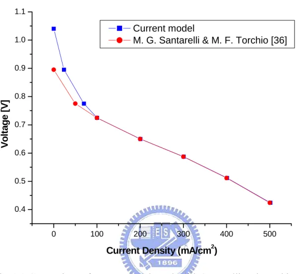
![Figure 4.1 shows the polarization curve of the reference case. With cell temperature of 353K, the reversible voltage is set to be 1.1154V by the equation obtained from reference [33]](https://thumb-ap.123doks.com/thumbv2/9libinfo/8736509.203212/64.892.130.806.104.368/figure-polarization-reference-temperature-reversible-equation-obtained-reference.webp)
