高速公路車流密度模式推估與模擬之研究

行政院國家科學委員會補助專題研究計畫成果報告

※※※※※※※※※※※※※※※※※※※※※※※※

※

※

※ 高速公路車流密度模式推估與模擬之研究 ※

※

※

※※※※※※※※※※※※※※※※※※※※※※※※

計畫類別：R個別型計畫 □整合型計畫

計畫編號：NSC89－2416－H－009－019－

執行期間：89年0月01日至90年07月31日

計畫主持人：周幼珍

共同主持人：

本成果報告包括以下應繳交之附件：

□赴國外出差或研習心得報告一份

□赴大陸地區出差或研習心得報告一份

□出席國際學術會議心得報告及發表之論文各一份

□國際合作研究計畫國外研究報告書一份

執行單位：國立交通大學統計研究所

中

華

民

國

90

年

10

月

31

日

行政院國家科學委員會專題研究計畫成果報告

高速公路車流密度模式推估與模擬之研究

計畫編號:NSC89-2416-H-009-019

執行期限:89年8月1日至90年7月31日

主持人:周幼珍

研究人員:

執行機構及單位:國立交通大學統計研究所

一、 中文摘要 本研究以隨機微分方程構建一隨機動態車流模 式以描述真實世界之隨機動態性, 另外, 模式的參數 估計方法為本研究另一重點, 儘管最大概似法(MLE) 是最常用的方法, 但所需要的最大概似函數僅有少 數模式可得[1], 有些研究指出可以用一般動差法 (generalized method of moments, GMM[2]) 來 估 計 , Gallant and Tauchen[1] 提出以有效動差法(efficient method of moments, EMM) 獲得估計函數, 在其研究 中, 亦證明有效動差法的計算效率與最大概似法相 近, 因此本研究中以有效動差法估計參數.

關鍵詞: 隨機微分方程, 動態車流模式, 一般動差 法, 有效動差法, 概似估計

Abstract

This project formulates a dynamic traffic flow model by a stochastic differential equation (SDE) to describe the real traffic phenomena on the roads. In addition, estimating the parameters of the model is another research topic herein. Although a maximum likelihood estimation (MLE) procedure is usually applied to estimate stochastic models, the exact solution and the likelihood function of a model are usually unknown except for only a few cases[1]. Some researchers suggest estimating the parameters by the generalized method of moments[2] (GMM). Furthermore, Gallant and Tauchen[1] proposed the efficient method of moments (EMM) to obtain the estimating function and proved that the estimators are as efficient as maximum likelihood estimation.

Keywords: stochastic differential equation, traffic flow, dynamic model, generalized method of moments, efficient method of moments, maximum likelihood estimation

二、Motivation and Objectives

Practical traffic systems in real world are stochastic as well as dynamic. Stochastic traffic flow models can be based on probabilistic distributions for lane-changing

and passing, traffic variables (headway, spacing, flow, and speed) distributions. Others are conducted according to queueing theory for signal control and intersection analysis or newly developed technologies such as particle hopping models that describes dynamic traffic phenomena or for special purposes such as incident detection. From previously studies, stochastic traffic models are mathematically complex. Deterministic results are obtained only where randomness vanishes but will remain a crude approximation since traffic is naturally random as previously mentioned.

According to mathematical modeling, a dynamic system with random fluctuations can be modeled by stochastic differential equations that involve stochastic processes as coefficients of the differential operator, as initial conditions, and as forcing functions. This work attempts to develop a stochastic differential model to represent stochastic dynamic traffic flow. The model is employed to describe time variant traffic flow on a freeway section that is under uninterrupted flow condition. In addition, the stochastic differential equation is (SDE) estimated by the efficient method of moments (EMM) herein[1, 3-6]. Real freeway data is employed as an example to illustrate EMM and show the accuracy.

三、Results and Discussions 3.1 Modeling

The stochastic time variant traffic flow is illustrated as

( ) ( ) ( )

t q t t

q = +ε , (1) where q

( )

t denotes traffic flow function that depends on time t and

(

)

T

M

1 q

q

q= ,..., , which is a M-dimensional variable. q

( )

t denotes time variant mean flow function and ε

( )

t denotes variance function, which is also time dependent. Flow changes with time is what we concern which is expressed as:

( )

t dt dq

( )

t dt d

( )

t dt

Let µ_t

( )

q,ρ =dq

( )

t dt , σ_t

( )

q,ρ =dε

( )

t dt , where

(

)

T p 1 ρ ρ =

ρ ,..., is a p-dimensional parameter vector. If

( )

ρ

σ_t q, (or dε

( )

t dt) is assumed to be a Wiener process,

( )

q dt

t ρ

σ , may be rewritten as σt

( )

q,tdWt, where W is a t

Wiener process. Equation (2) can be converted into Itoˆ

form as follows:

( )

( )

( )

1 mt m M t 1 M t 1 M W d q dt q t q d × × × × =µ ,ρ +σ ,ρ , (3) where

( )

(

( )

( )

)

T Mt t 1 t ⋅ρ = µ ⋅ρ µ ⋅ρ µ , , ,..., , is a M-dimensional drift function (or mean function) that represents instantaneous mean of the state variable and

( )

(

( )

( )

)

T Mt t 1 t ⋅ρ = B ⋅ρ B ⋅ρ σ , , ,..., , is a M×m-dimensional drift function (or variance function) that represents instantaneous variance of the state variable.

3.2 Estimation method

The explicit solution of Eq. (3) can be represented as

( )

_∫

(

( )

)

_∑∫

(

( )

)

= ρ σ + ρ µ + = m 1 i s 0 is is t 0 s 0 qs ds qs dW q t q , , , (4 ) where

∫

s_σ

(

( )

_ρ

)

0 is q s, dWis

denotes Itoˆ stochastic integral. However, for a stochastic differential equation, even q

( )

t can be detected in continuous time interval

[ ]

0T

t∈ , there are only a few models can be directly solved by a maximum likelihood estimator (MLE). In stead of MLE, GMM provides an estimation process to estimate parameters of a structural model without a specific density function, which is necessary of MLE. Thus, Gallant and Tauchen[1] presented a systematic approach to generate moment conditions for GMM estimator of the parameters of a structural model which is termed as efficient method of moments (EMM). The basic idea is to employ an auxiliary model (score generator) to obtain the expected scores of a structural model and treat them as the moment conditions. The parameter estimation process is illustrated as follows: (1) Establish a score generator by the SNP method

A score generator must first be obtained. If the process

{ }

q

_t is correctly described by the density

(

q−L q0ρ

)

p ,..., introduced by the stochastic differential equations and by some other time invariant density

(

q−L q0θ

)

f ,..., , which is the score generator as defined before. Then let

(

)

₍

(

₎

)

∫

θ θ = θ − − − t L t t L t t 1 t t dq q q f q q f x q f ,..., ,..., , , (5) where

(

)

1 t L t 1 t q q

x₋ = ₋ ,..., ₋ . A score generator is obtained and does not have to employ SNP method[1, 7]. If the distribution of the process

{ }

q_t is unknown, a score generator should be computed by the SNP method. First, it is assumed that the expectation of score depends on the lagged variables.

( )

t L t T x

q = ₊ t=−L,−L+1,... (6) of the state are recorded, where

t

q denotes an M-dimensional vector that is a random variable,

(

t L

)

x

x_t+L= + denotes the lagged variable that is M⋅L long and L≥0 denotes the number of lagged variables. Then, the SNP estimator is illustrated as

(

q_t x,θ

)

∝

[

P

( )

z,x

]

2N_M

(

qµ_x,Σ

)

f , (7) where x t t Rz q = +µ ,

(

)

1 t 1 0 1 t t x =Eq x− =b +bx− µ ,

(

_T

)

T 1 t T 1 L t T L t 1 t q q q x₋ = ₋ , _{− −},..., ₋ , P ,

( )

z x denotes a multivariate polynomial of degree K_z and the coefficients are

x

_t , which are the K_x degrees polynomial of historical data. Thus,

( )

_∑∑

= = α = Kz x 0 i K 0 j j i ijzx x z P , (8) is a polynomial of degree K_z+K_x.

The variance-covariance matrix is assumed to depend on historical data to represent conditional heterogeneity. Let R be a linear of the absolute values of the vector elements qt−Lr −µxt−1−Lrthrough qt−1−µxt−2

and the variance-covariance matrix Σ_x becomes T x xR

R . The variance function is denoted as:

( )

_∑

= −− + −− + − =ρ + −µ r i r L 2 t r 1 t L 1 i x i L 1 t i 0 x P q R vech , (9)

where vech

( )

R denotes a M

(

M+1

)

2 long vector that contains the elements of the upper triangle of the R matrix,

0

ρ is a M

(

M+1

)

2 long vector, P through ₁

r

L

P are M

(

M+1

)

2 by M matrices, and q−µ denotes a vector that contains the absolute values of q−µ. Lu

denotes the number of lags in µx, L denotes the r

number of lags in vech(R), L denotes the number of p

lags of x part of the polynomial P ,

( )

z x , and L is the total number of lags under consideration

(

Lp Lu Lr Lu

)

L=max , , + .

Therefore, to obtain the SNP estimator, the parameters of the three parts described below must be determined by the empirical traffic data. The first part is the parameters of the mean function,

∑

= − + = µ L 1 i i t i 0 x b bx i=1,2,...L t=1,...,T (10) are denoted by

[

]

i 0 b b

Ψ , which is a Gaussian VAR. The second part is the parameters of the variance function Eq.(11) which are denoted by τ

[ ]

ρ₀P_i , which is a Gaussian VAR+VRCH. The third part is the parameters of the Hermite polynomial Eq.(8), which is denoted by A(

ij

α ).

Let

θ

=

[_AΨτ], which is estimated by θˆ , be _T obtained by minimizing

( )

_∑

(

)

= − θ       − = θ T 1 t 1 t t T T f q x T 1 s ˆ log , . (9) That is

(

)

∑

= − Θ ∈ θ  θ     − = θ T 1 t 1 t t T f q x T 1 , log max arg ˆ . (10)

However, there are lagged number that must be determined to ascertain the mean function, the variance function and the Hermite polynomial. The conventional selection criteria employed are AIC[8], BIC[9] and HQC[10]. BIC is conservative as it selects sparser parameterizations than the AIC. HQC falls between these two extremes. Gallant and Tauchen[7] suggested using BIC to move along an upward expansion path until an adequate model is determined.

(3) Compute the information matrix of a score generator and generate moment conditions

The maximum likelihood estimation theory produces the following two mathematical results:

( )

{

qtxt1 K

}

p(qt L qt )dqtL dqt f 0 L ₋ ρ ₋ ρ ₋ L θ ∂ ∂ ≡

_{∫ ∫}

log , ,..., , , (11) ( )

{

}

{

( )

}

( ) ( )

{

t t

}

(tL t ) tL t T t L t t L t T t t t t dq dq q q p K x q f dq dq q q p K x q f K x q f I L L L L − − − − − − −

∫ ∫

∫ ∫

∂ ∂ ∂ − = ×     ∂ ∂     ∂ ∂ = ρ ρ θ θ ρ ρ θ ρ θ , ,..., , log , ,..., , log , log 1 2 1 1 (12)

Therefore, to the first order, minimizing

( )

{

θ −_Kρ

}

_I−

{

θ −_K

( )

ρ

}

T 1 T T T ˆ

ˆ _{is the same as minimizing}

( )

[

]

N

( )

T 1 T T T N I h h ρ,θˆ − ρ,θˆ . h

( )

ρ,θ may be computed by averaging a long simulation:

( )

∑

{

}

= − − θ θ ∂ ∂ ≈ θ ρ N 1 t T 1 t L t t T N f q q q N 1 h ,ˆ log ˆ ˆ ,...,ˆ ,ˆ . (13)

As sample size N is large enough, Eq. (13) can approximate to Eq. (12). The approximation is so called Monte Carlo integral.

(4) Employ the GMM estimator to estimate ρ The GMM estimator ρˆ is

( )

[

]

N

( )

T 1 T T T N R h I h ρθ ρθ = ρ − ∈ ρ ˆ , ˆ , max arg ˆ . (14)

The (estimated) asymptotic covariance matrix of the EMM estimator ρˆ is

( )

1

(

( )

_ˆ

)

1 ˆ = _ρ θ _ρ − ρ H I H T Cov T T T , (15) where _ρ=

(

_∂

( )

_{ρθ ∂ρ}

)

T N h

H ˆ,ˆ and the minimized value of T

times EMM criterion function is distributed as _χ2 _with

( )

θˆ −dim

( )

ρˆ

dim _T degrees of freedom, where dim

( )

ρˆ denotes the number of elements in the vector ρˆ , if the structural model is correctly specified.

3.3Empirical study

The data set was collected from the No. 3 National Freeway north bound 86 km on 16 February 1999. Table 1 lists the statistics values obtained from the SAS. Normal distribution is treated as a basis and the skewness and kurtosis are modified by the Hermite polynomial to make the data fit the distribution in the SNP.

Using BIC to move along an upward expansion path until an adequate set of lagged numbers is obtained.

3

L_u = minimizes AIC, BIC, and HQC. Although 7

L_r = minimizes AIC and HQC, BIC utilizes L_r =3 because both AIC and HQC selected too many variables. According to the selection criterion table, K_z=3 and

0

Kx= are chosen which induces P ,

( )

z x to be a third

order polynomial of z. _{K 0}

x = means that the

coefficients are independent to historical data. Table 1 The output of empirical data from SAS

Moments N 288 Sum Wgts 288 Mean 130.5451 Sum 37597 Std Dev 76.34315 Variance 5828.277 Skewness 0.190541 Kurtosis -0.95643 USS 6580821 Css 1672715 CV 58.48027 Std Mean 4.498563 T:Mean=0 29.0193 Pr > |T| 0.0001 Num=0 288 Num>0 288 M(sign) 144 Pr >= |M| 0.0001 Sgn Rank 20808 Pr >= |S| 0.0001

Thus, the score generator obtained by SNP is illustrated as:

(

)

(

)

(

2

)

x x 2 3 3 2 2 1 0 t z z z Nq x q f ,θ ∝ α +α +α +α µ ,σ , (16) where 3 t 3 2 t 2 1 t 1 0 x =b +bq− +b q− +b q− µ , (17) 4 t 3 t 2 t 2 t2 x 3 t3 x x 1 t 1 0 x=ρ +ρ q −µ − +ρ q −µ − +ρ q −µ − σ − − − . (18)

In the SNP, considering the round-off computational error,

( )

0

x z

P , +ε is substituted for P ,

( )

z x so the score becomes:

(

)

{

[

[

_[

_{( )}

]

_{] ( )}

]

}

(

)

0 2 2 x x m 0 2 x 1 x ds s x s P q N x q P x q f ε + φ σ µ ε + µ − σ = θ

∫

− , , , , , (19) where ₀₀₀₁ 0 = .

ε . Table 2 is the estimation results from the lagged numbers L_u =3,L_r =3,K_z =3.

Generating the moment condition is the next step in the estimation. Let N=10,000 to simulate

(

qt ρ

)

=α1+β1⋅qt

µ , and σ

(

qt,ρ

)

=α2 +β2⋅qt are

chosen. The chi-square is _χ2

( )

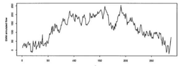
7 ₌10_.269 _{, which} indicates that the structural model is acceptable. Tables 3 and 4 are the estimation results of the parameters of and the t-statistics, which confirm the parameters are reasonable and significant. Figure 1 is the actual data while Figure 2 displays the estimation results.

This study constructs a stochastic model to represent the time variant traffic flow and employs EMM method to estimate the parameters since EMM can efficiently estimate the parameters of the structural model. There are several aspects leaving to further research. In the estimation procedure, the moment condition, _h

( )

_ρ,θˆ, is estimated by

( )

_ρ,θˆ

N

h as N is large enough. However, different N produces distinct results. In addition, the computation becomes more complex as

N increases. Therefore, how to determine an appropriate N is an important further research topic.

Table 2. The estimated parameters

parameters standard deviation t-ratio

2 A 0.14693 0.06659 2.206 3 A -0.20018 0.03863 -5.182 4 A -0.04053 0.01985 -2.042 1 Ψ -0.05575 0.01176 -4.740 2 Ψ 0.25639 0.05645 4.542 3 Ψ 0.35327 0.04782 7.388 4 Ψ 0.34106 0.04599 7.415 1 τ 0.13949 0.02574 5.419 2 τ 0.68111 0.10486 6.495 3 τ 0.14032 0.09720 1.444 4 τ 0.46823 0.09284 5.043

Table 3. The scores and the statistical results

Scores s. d. t-ratio 2 A 3.02727 2.14400 1.412 3 A 3.98679 3.26852 1.220 4 A 3.66721 6.59742 0.558 1 Ψ 10.42392 5.90399 1.766 2 Ψ -9.16756 7.08964 -1.293 3 Ψ -6.77414 7.60898 -0.890 4 Ψ -10.15077 7.52577 -1.349 1 τ 6.91288 5.88235 1.175 2 τ 1.01630 1.13576 0.895 3 τ 1.42067 1.13618 1.250 4 τ 1.55554 0.79777 1.950

Table 4. The estimated SDE parameters

parameters s. d. t-ratio 1 α 0.00059392 0.00010683 5.55944064 1 β -0.02288550 0.00022580 -101.35310724 2 α 0.08606748 0.00011783 730.45189614 2 β -0.00262145 0.00010331 -25.37424970

Figure 1 The observation data of traffic flow

Figure 2 The estimation result of traffic flow 四、Comments

This work is based on the stochastic differential equation and the efficient method of moment. We successfully develop the stochastic dynamic traffic flow model and estimate the parameters. The empirical study shows that the methodology is available for forecasting traffic flow. Hence, the result coincides to the objectives and the expected result. In addition, the result is also submitted to the international journal (Transportation Technology and Planning).

五、References

1. A. R. Gallant and G. Tauchen, Which Moments to Match, Eco. Theory, 15, 657-681, (1996). 2. L. P. Hansen, Large Sample Properties of

Generalized Method of Moments Estimators, Econometrica, 50, 1029-1054, (1982).

3. J. C. Cox, J. E. Ingersoll Jr. and S. A. Ross, A Theory of the Term Structure of Interest Rates, Econometrica, 53, 385-407, (1985).

4. K. C. Chan, G. A. Karolyi, F. A. Longstaff, and A. B. Sanders, An Empirical Comparison of Alternative Models of Short-Term Interest Rates, The Journal of Finance, 107, 1209-1227, (1992).

5. R. A. Bansal, A. Gallant, R. Hussey and G. Tauchen,

Non-Parametric Estimation of Structural Models for High-Frequency Currency Market Data, J. of Econometrics, 66, 251-287, (1995).

6. Y. Ait-Sahalia, , Nonparametric Pricing of Interest Rate Derivative Securities, Econometrica, 64, 527-560, (1996).

7. A. R. Gallant and G. Tauchen, SNP: A Program for Nonparametric Time Series Analysis Version 8.7 User Guide, 1998.

8. H. Akaike, Fitting Autoregressive Models for Prediction, Annals of the Institute of Statistical Mathematics, 21, 243-247, (1969).

9. G. Schwarz, Estimating the Dimension of a Model, Annals of Statistics, 6, 461-464, (1978).

10. E. J. Hannan, Rational Transfer Function Approximation, Statistical Science, 2, 1029-1054, (1987).