VOLUME86, NUMBER16 P H Y S I C A L R E V I E W L E T T E R S 16 APRIL2001
Precision Calculation of Magnetization and Specific Heat of Vortex Liquids and Solids
in Type-II Superconductors
Dingping Li and Baruch Rosenstein
National Center for Theoretical Sciences and Electrophysics Department, National Chiao Tung University, Hsinchu 30050, Taiwan, Republic of China
(Received 5 July 2000)
A new systematic calculation of magnetization and specific heat contributions of vortex liquids and solids is presented. We develop an optimized perturbation theory for the Ginzburg-Landau description of thermal fluctuations effects in the vortex liquids. The expansion is convergent in contrast to the conventional high temperature expansion which is asymptotic. In the solid phase we calculate the first two orders which are already quite accurate. The results are in good agreement with existing Monte Carlo simulations and experiments. Limitations of various nonperturbative and phenomenological approaches are noted. In particular, we show that there is no exact intersection point of the magnetization curves.
DOI: 10.1103/PhysRevLett.86.3618 PACS numbers: 74.60. – w, 74.20.De, 74.25.Dw, 74.25.Ha
It was clearly seen in both magnetization [1] and spe-cific heat experiments [2] that thermal fluctuations in high
Tc superconductors are strong enough to melt the vortex
lattice into liquid over large portions of the phase dia-gram. The transition line between the Abrikosov vortex lattice and the liquid is located far below the mean field phase transition line. Between the mean field transition line and the melting point physical quantities like the mag-netization, conductivity, and specific heat depend strongly on fluctuations. Several experimental observations call for a refined precise theory. For example, a striking fea-ture of magnetization curves intersecting at the same point 共Tⴱ, Hⴱ兲 was observed in a wide rage of magnetic fields in both the layered [3] materials and the more isotropic ones [4]. To develop a quantitative theory of these fluctuations, even in the case of the lowest Landau level (LLL) corre-sponding to regions of the phase diagram “close” to Hc2
[5], is a very nontrivial task and several approaches were developed.
Thouless and Ruggeri [6] proposed a perturbative ex-pansion around a homogeneous (liquid) state in which all the “bubble” diagrams are resummed. Unfortunately, they proved that the series is asymptotic and although the first few terms provide accurate results at very high temperatures, the series becomes inapplicable for LLL dimensionless temperature aT ⬃ 关T 2 Tmf共H兲兴兾共TH兲1兾2
smaller than 2 in 2D quite far above the melting line (be-lieved to be located around aT 苷 212). Generally,
at-tempts to extend the theory to lower temperatures by the Borel transform or Pade extrapolation were not successful [7]. Several nonperturbative methods have also been at-tempted including renormalization group [8] and the 1兾N expansion [9]. Tesanovic and co-workers developed a the-ory based on separation of the two energy scales [10]: the condensation energy (98%) and the motion of the vortices (2%). The theory explains the intersection of the magneti-zation curves.
In the first part of this paper we apply optimized pertur-bation theory (OPT) first developed in field theory [11,12] to both the 2D and 3D LLL model. It allows one to ob-tain a convergent (rather than asymptotic) series for mag-netization and specific heat of vortex liquids together with precision estimate. The radius of convergence is aT 苷 23
in 2D and aT 苷 25 in 3D. On the basis of this one can
make several definitive qualitative conclusions.
Our starting point is the Ginzburg-Landau free energy:
F 苷 Lc Z d2x h¯ 2 2mjDcj 2 1 ajcj21 b 0 2 jcj 4, (1) where A苷 共By, 0兲 describes a nonfluctuating constant magnetic field in Landau gauge and D ⬅ = 2 i2pF
0A,
F0 ⬅
hc
2e, Lc is the width (for simplicity we write
ex-pressions for the 2D case, essential 3D complications are discussed separately). For simplicity we assume
a共T兲 苷 aTc共1 2 t兲, t ⬅ T兾Tc. On LLL, the model after
rescaling reduces to f 苷 1 4p Z d2x ∑ aTjcj21 1 2 jcj 4 ∏ , (2)
where the LLL reduced temperature aT ⬅ 2
q 4p
bv
12t2b 2 is the only parameter in the theory [6]. Here b ⬅ HB
c2,
v ⬅ 共32p3e2k2j2T兲兾共c2h2L
z兲.
We will use a version of OPT, the optimized Gaussian series [12]. It is based on the “principle of minimal sen-sitivity” idea [11], first introduced in quantum mechanics. Generally a perturbation theory starts from dividing the Hamiltonian into a solvable “large” part K and a perturba-tion V . Since we can solve any quadratic Hamiltonian we have a freedom to choose “the best” such quadratic part. Quite generally such an optimization converts an asymp-totic series into a convergent one (see a comprehensive discussion, references, and a proof in [12]).
VOLUME86, NUMBER16 P H Y S I C A L R E V I E W L E T T E R S 16 APRIL2001 Because of the translational symmetry of the vortex
liq-uid there is just one variational parameter ´ in the free energy divided as follows:
K 苷 ´ 4p jcj 2 , V 苷 1 4p ∑ aHjcj21 1 2 jcj 4 ∏ , (3) where aH ⬅ aT 2 ´. One reads Feynman rules from
Eq. (3): K determines the propagator (just a constant), the first term in V is a “mass insertion” vertex with a value of
1
4paH, while the four line vertex is 8p1 . To calculate the effective free energy density feff 苷 24p lnZ, one draws all the connected vacuum diagrams. We calculated directly diagrams up to the three loop order. However, to take advantage of the existing long series of the nonopti-mized Gaussian expansion, we found a relation of the OPT to this series. Originally Thouless and Ruggeri calculated this series feff to sixth order, but it was sub-sequently extended to 12th (9th in 3D) by Brezin et al. and to 13th by Hu et al. [13]. It is usually presented using variable x introduced by Thouless and Ruggeri [6] x 苷 ´12, ´苷 1 2共aT 1 p a2 T 1 16兲 as follows: feff 苷 2 log4p´2 1 2 P`
n苷1cnxn. We can obtain all the OPT
diagrams which do not appear in the Gaussian theory by insertions of bubbles and mass insertions from the dia-grams contributing to the nonoptimized theory. Bubbles or “cacti” diagrams are effectively inserted by a technique known in field theory [14]:
feff 苷 2 log ´1 4p2 1 2 ` X n苷1 cnxn, x苷 a ´21 , ´1 苷 1 2 共´2 1 p ´2 21 16a兲 . (4)
Summing up all the insertions of the mass vertex is achieved by ´2 苷 ´ 1 aaH. Here a was introduced
to keep track of the order of the perturbation, so that expanding feff to order an11, and then taking a 苷 1 we obtain ˜fn共´兲 (calculating ˜fn that way, we checked that
indeed the first three orders agree with the direct cal-culation). The nth OPT approximant fn is obtained by
minimization of ˜fn共´兲 with respect to ´:
µ ≠ ≠´ 2 ≠ ≠aH ∂ ˜ fn共´, aH兲 苷 0 . (5)
The above equation is equal to 1兾´2n13 times a polyno-mial gn共z兲 of order n in z ⬅ ´aH. That Eq. (5) is of this
type can be seen by noting that the function f depends on the combination a兾共´ 1 aaH兲2only. We were unable
to prove this, but have checked it to the 40th order. This property greatly simplifies the task: one has to find roots of polynomials rather than solving transcendental equations. There are n (real or complex) solutions for gn共z兲 苷 0.
However (as in the case of anharmonic oscillator [12]), the best results give a real root with the smallest abso-lute value. We then obtain ´共aT兲 苷 12共aT 1
p
aT2 2 4zn兲
solving zn 苷 ´aH 苷 ´aT 2 ´2.
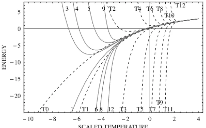
In Fig. 1 we present OPT for different orders including
n苷 0 (Gaussian) together with several orders of the
− 10 − 8 − 6 − 4 − 2 0 2 4 SCALED TEMPERATURE − 20 − 15 − 10 − 5 0 5 ENERGY 3 4 5 9 T2 T4 T6 T8 T10 T12 T11 T9 T7 T5 T3 12 8 6 T1 1 T0
FIG. 1. Optimized (solid lines) and nonoptimized (dashed lines) free energy approximants in 2D. Numbers indicate the order of the approximant.
nonoptimized high temperature expansion. One observes that the OPT series converges above aT 苷 22.5 and
diverges below aT 苷 23.5. The proof of convergence
is analogous to that for the anharmonic oscillator; see Ref. [12]. On the other hand, the nonoptimized series never converges despite the fact that above aT 苷 2
the first few approximants provide a precise estimate consistent with OPT. Above aT 苷 3 the liquid becomes
essentially a normal metal and fluctuations effects are negligible (see Figs. 2 and 3). Therefore the information the OPT provides is essential to compare with experi-ments on magnetization and specific heat. If precision is defined as共 f12 2 f10兲兾f10, we obtain 4.87%, 1.27%, 0.387%, 0.222%, 0.032% at aT 苷 22, 21.5, 21, 20.5, 0,
respectively. For comparison with other theories and experiments in Figs. 2 and 3 we use the 10th approximant. The calculation is basically the same in 3D, the only complication being extra integrations over momenta par-allel to the magnetic field. However, since the propagator factorizes, these integrations can be reduced to correspond-ing integrations in quantum mechanics of the anharmonic oscillator [6,11]. The series converges above aT 苷 24.5
and diverges below aT 苷 25.5. The nonoptimized series
is useful only above aT 苷 21. The agreement is within
− 7.5 − 5 − 2.5 0 2.5 5 7.5 10 SCALED TEMPERATURE − 7 − 6 − 5 − 4 − 3 − 2 − 1 0 MA GNETIZA TION OPT theory eq.10 theory eq.9 exp. 0.5 T exp. 1 T
FIG. 2. The 2D scaled LLL magnetization. Comparison of data from Jin et al. in Ref. [3] with OPT calculation, Tesanovic et al. result of Ref. [10] [Eq. (9)] and phenomenological “inter-ception” theory Eq. (10) are shown for comparison.
VOLUME86, NUMBER16 P H Y S I C A L R E V I E W L E T T E R S 16 APRIL2001
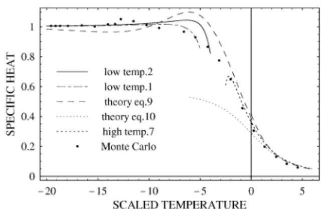
FIG. 3. Specific heat, 2D. Comparison of MC data with solid OPT (first two orders), liquid OPT (10th order). Tesanovic et al. theory and phenomenological formula are also shown.
the expected precision when we compare our results in 3D with Ref. [15].
Now we turn to the vortex solids. Here the minimization is significantly more difficult due to reduced symmetry. Unlike in the liquid the field c acquires a nonhomogeneous expectation value and can be expressed as c共x兲 苷 y共x兲 1
x共x兲, where x describes fluctuations. Assuming hexago-nal symmetry, it should be proportiohexago-nal to the mean field solution y共x兲 苷 ywk苷0共x兲 with a variational parameter
y taken real thanks global U共1兲 gauge symmetry where wk共x兲 is the quasimomentum basis on LLL [5].
Expand-ing x
x共x兲 苷 1 2pp2
Z
k
exp关2iuk兾2兴wk共x兲 共Ok 1 iAk兲 , (6)
where real fields Ak 苷 Aⴱ2k 共Ok 苷 O2kⴱ 兲 describe acous-tic (opacous-tical) phonons of the flux latacous-tice. The phase exp关2iuk兾2兴 defined, as in the low temperature
per-turbation theory developed recently [16], via gk 苷
jgkj exp关iuk兴, gk ⬅ 具w0共x兲w0共x兲wkⴱ共x兲wⴱk共x兲典x, is crucial
for simplification of the problem. The most general quadratic form is K 苷 1 8p Z k OkGOO21共k兲O2k 1 AkGAA21共k兲A2k 1 OkGOA21共k兲A2k 1 AkGOA21共k兲O2k, (7) with matrix of functions G共k兲 to be determined together with the constant y by the variational principle. The cor-responding Gaussian free energy feff is
aTy21 bA 2 y 4 2 2 2 具log关共4p兲2det共G兲兴 2 aT关GOO共k兲 1 GAA共k兲兴典k 1具y2关共2bk 1 jgkj兲GOO共k兲 1 共2bk 2 jgkj兲GAA共k兲兴典k 1具bk2l关GOO共k兲 1 GAA共k兲兴 关GOO共l兲 1 GAA共l兲兴典k,l 1 1 2bA 兵具jgkj关GOO共k兲 2 GAA共k兲兴典k2 1 4具jgkjGOA共k兲典2k其 ,
where具· · ·典kdenotes the average over Brillouin zone bk ⬅
具wⴱ0共x兲w0共x兲wkⴱ共x兲wk共x兲典x, bA 苷 b0. The gap equations obtained by the minimization of the free energy look quite intractable, however, they can be simplified. The crucial observation is that GOA共k兲 苷 0 is a solution, and the
gen-eral solution can be shown to differ from this simple one just by a global gauge transformation. One can set matrix
G21 as µ E共k兲 1 Djgkj 0 0 E共k兲 2 Djgkj ∂ ,
where D is a constant (details will appear elsewhere). The function E共k兲 and the constant D satisfy
E共k兲 苷 aT 1 2y2bk 1 2 ø bk2l µ 1 EO共l兲 1 1 EA共l兲 ∂¿ l , bAD苷 aT 2 2 ø bk µ 1 EO共k兲 1 1 EA共k兲 ∂¿ k . (8)
Observing that bk has a very effective expansion in
x ⬅ exp关2a2D兾2兴 苷 exp关22p兾 p 3兴 苷 0.0265, bk 苷 P` n苷0xnbn共k兲, bn共k兲 ⬅ P jXj2苷na2
Dexp关ik ? X兴 and
us-ing the hexagonal symmetry of the spectrum, E共k兲 can also be expanded in “modes” E共k兲 苷PEnbn共k兲. The integer
n determines the distance of a points on the hexagonal lattice X from the origin. One estimates that En ⯝ xnaT,
therefore the coefficients decrease exponentially with n. For some integers, for example, n 苷 2, 5, 6, bn 苷 0. We
minimized numerically the Gaussian energy by varying y, D, and the first few modes of E共k兲. In practice two modes are quite enough. The results show that around
aT , 25, the Gaussian liquid energy is larger than the
Gaussian solid energy. So naturally when aT , 25, one
should use the Gaussian solid to set up a perturbation theory instead of the liquid one. The Gaussian energy in either liquid (see line T0 on Fig. 1) or solid is a rigorous upper bound on the free energy. We calculated the leading correction (without its minimization) in order to determine the precision of the Gaussian result (see Fig. 3 for the specific heat results). We obtain 0.2%, 0.4%, and 2% at
aT 苷 230, 220, 212, respectively.
In the rest of the paper we compare our results with other theories, simulations, and experiments. An analytic theory used successfully to fit the magnetization and the specific heat data [17]was developed in [10]. Their free energy density is feff 苷 2 a2TU2 4 1 aTU 2 s U2a2 T 4 1 2 1 2 arcsinh ∑ aTU 2p2 ∏ , U 苷 1 2 ∑ 1 p 2 1 1 p bA (9) 1 tanh ∑ aT 4p2 1 1 2 ∏ µ 1 p 2 2 1 p bA ∂∏ . 3620
VOLUME86, NUMBER16 P H Y S I C A L R E V I E W L E T T E R S 16 APRIL2001 The corresponding magnetization and specific heat are
shown as dashed lines in Figs. 2 and 3, respectively. At large positive aT, feff 苷 2 logaT 1
4 a2T 2 16 aT4 1 320 3a6T and differs very little from the exact series 2 logaT 1
4 a2T 2 18 a4T 1 1324 9aT6
. Its low temperature asymptotics is, however, less precise: 2 a
2 T
2bA 2 2 log
jaTj
4p2, which has an opposite
sign of the log term compared to the exact series [16] 2 a 2 T 2bA 1 2 log jaTj 4p2 2 19.9 a2
T . This is seen in Fig. 3 quite
clearly. Instead of rising monotonously from C兾DC 苷 1 until melting as is predicted by OPT, their curve (dashed) first drops below 1 and only later develops a maximum above 1. In the liquid region it underestimates the specific heat. We conclude therefore that although the theory of Tesanovic et al. is very good at high temperatures they be-come of the order 5–10% at aT 苷 23. An advantage of
this theory is that it interpolates smoothly to the solid and never deviates more than 10%.
Experiments on a great variety of layered high Tc
cuprates (Bi or Tl [3] based) show that in 2D, magne-tization curves for different applied fields intersect at a single point 共Mⴱ, Tⴱ兲. The range of magnetic fields is surprisingly large (from several hundred Oe to several Tesla). This property fixes the scaled LLL magnetization defined as m共aT兲 苷 2 dfeff共aT兲 daT 苷 mab eⴱh q 4p bvM. Demanding
that the first two terms in 1兾aT2 expansion of m共aT兲 are
consistent with the exact result, one obtains
m共aT兲 苷
1 4 共aT 2
q
16 1 aT2兲 . (10)
When it is plotted in Fig. 2 (the dotted line), we find that at lower temperatures the magnetization is overestimated. The OPE results are consistent with the experimental data [3] (points) within the precision range until the radius of convergence aT 苷 23. It is important to note that
devia-tions of both the phenomenological formula Eq. (10) and Tesanovic’s are clearly beyond our error bars. Therefore we conclude that the coincidence of the intersection of all the lines at the same point共Tⴱ, Mⴱ兲 cannot be exact. As in 3D the intersection is approximate, although the approxi-mation is quite good especially at high magnetic fields.
Specific heat OPE results in 2D is compared in Fig. 3 with Monte Carlo simulation of the same model by Kato and Nagaosa [18] (black circles) [and the phenomenologi-cal formula following from Eq. (10), dotted line]. The agreement is very good for both the low temperature and the high temperature OPT.
To summarize, we obtained the optimized perturbation theory results for the 2D and 3D LLL Ginzburg-Landau model in both vortex liquid and solid phases. The leading approximant (Gaussian) gives a rigorous upper bound on energy, while the convergent series allows one to make several definitive qualitative conclusions. The intersection of the magnetization lines is only approximate not only in
3D, but also in 2D. The theory by Tesanovic [10] describes the physics remarkably well at very high temperatures, but deviates on the 5%–10% precision level at aT 苷 22 in
2D and has certain imprecise qualitative features in the solid phase. Comparison with Monte Carlo simulations and some experiments shows excellent agreement.
We are grateful to our colleagues A. Knigavko and T. K. Lee for numerous discussions and encouragement and to Z. Tesanovic for explaining his work to one of us and sharing his insight. The work was supported by NSC of Taiwan Grant No. 89-2112-M-009-039.
[1] E. Zeldov, D. Majer, M. Konczykowski, V. B. Geshkenbein, V. M. Vinokur, and H. Shtrikman, Nature (London) 375,
373 (1995).
[2] M. Roulin, A. Junod, A. Erb, and E. Walker, J. Low Temp. Phys. 105,1099 (1996); A. Schilling et al., Phys. Rev. Lett. 78,4833 (1997).
[3] R. Jin, A. Schilling, and H. R. Ott, Phys. Rev. B 49,9218 (1994); P. H. Kes et al., Phys. Rev. Lett. 67,2383 (1991); A. Wahl et al., Phys. Rev. B 51,9123 (1995).
[4] U. Welp et al., Phys. Rev. Lett. 67,3563 (1991).
[5] For discussion of the range of applicability, see D. Li and B. Rosenstein, Phys. Rev. B 60,9704 (1999).
[6] D. J. Thouless, Phys. Rev. Lett. 34, 946 (1975); G. J. Ruggeri and D. J. Thouless, J. Phys. F 6,2063 (1976). [7] G. J. Ruggeri, Phys. Rev. B 20,3626 (1979); N. K. Wilkin
and M. A. Moore, Phys. Rev. B 47,957 (1993).
[8] E. Brezin, D. R. Nelson, and A. Thiaville, Phys. Rev. B 31,
7124 (1985); T. J. Newman and M. A. Moore, Phys. Rev. B 54,6661 (1996).
[9] I. Affleck and E. Brezin, Nucl. Phys. B257,451 (1985); M. A. Moore, T. J. Newman, A. J. Bray, and S-K. Chin, Phys. Rev. B 58,936 (1998); A. Lopatin and G. Kotliar, Phys. Rev. B 59,3879 (1999).
[10] Z. Tesanovic, L. Xing, L. Bulaevskii, Q. Li, and M. Suenaga, Phys. Rev. Lett. 69, 3563 (1992); Z. Tesa-novic and A. V. Andreev, Phys. Rev. B 49,4064 (1994). [11] P. M. Stevenson, Phys. Rev. D 32,1389 (1985); A.
Okopin-ska, Phys. Rev. D 35,1835 (1987).
[12] H. Kleinert, Path Integrals in Quantum Mechanics, Sta-tistics, and Polymer Physics (World Scientific, Singapore, 1995).
[13] E. Brezin, A. Fujita, and S. Hikami, Phys. Rev. Lett. 65,
1949 (1990); S. Hikami, A. Fujita, and A. I. Larkin, Phys. Rev. B 44, 10 400 (1991); J. Hu, A. H. MacDonald, and B. D. McKay, Phys. Rev. B 49,15 263 (1994).
[14] T. Barnes and G. I. Ghandour, Phys. Rev. D 22,924 (1980); A. Kovner and B. Rosenstein, Phys. Rev. D 39, 2332 (1989); 40,504 (1989).
[15] R. Sasik and D. Stroud, Phys. Rev. Lett. 75,2582 (1995). [16] B. Rosenstein, Phys. Rev. B 60,4268 (1999); H. C. Kao, B. Rosenstein, and J. C. Lee, Phys. Rev. B 61, 12 352 (2000).
[17] S. W. Pierson, O. T. Valls, Z. Tesanovic, and M. A. Linde-mann, Phys. Rev. B 57, 8622 (1998); S. W. Pierson and O. T. Valls, Phys. Rev. B 57,8143 (1998).
[18] Y. Kato and N. Nagaosa, Phys. Rev. B 48, 7383 (1993); J. Hu and A. H. Mcdonald, Phys. Rev. Lett. 71,432 (1993).