科技部補助專題研究計畫成果報告
期末報告
外部經濟與都市分佈
計 畫 類 別 : 個別型計畫 計 畫 編 號 : MOST 104-2410-H-004-200-執 行 期 間 : 104年08月01日至106年07月31日 執 行 單 位 : 國立政治大學經濟學系 計 畫 主 持 人 : 陳心蘋 共 同 主 持 人 : 陳心蘋、廖郁萍 計畫參與人員: 碩士班研究生-兼任助理:彭思瑾 碩士班研究生-兼任助理:郭獻聰 碩士班研究生-兼任助理:王靖筑中 華 民 國 106 年 06 月 29 日
中 文 摘 要 : Eeckhout (2004)提出的外部經濟的一般均衡理論可解釋都市的人口 分布以及都市成長的特質。模型中的生產力參數與地方外部性是推 導出都市人口分布以及都市人口成長特質的關鍵。本研究的目的是 探討生產力參數與地方外部性如何影響人口成長率;這兩個變數如 何影響都市人口分布;以及人口的極限分布情形。研究結果顯示 ,在控制了外生技術衝擊變數的分布特質下,此理論可推導出對數 常態分布。在特定的外生技術衝擊變數範圍內,以及負的地方外部 效果條件下,都市人口成長率與外生技術衝擊變數成正向相關。在 同樣的外生技術衝擊變數下,地方外部效果的絕對值越大,都市人 口成長率越小。當地方外部效果的絕對值遞減時,吉尼係數遞增。 地方外部效果的絕對值越小,都市人口越集中分佈。外生技術衝擊 變數分佈的標準差越大,吉尼係數越大,表示外生技術衝擊變數越 分散,都市人口分佈越集中。 中 文 關 鍵 詞 : 關鍵字:地方外部性、產出的都市人口彈性、外生技術衝擊變數 英 文 摘 要 : An equilibrium theory of local externalities proposed in Eeckhout (2004) explains both empirical size distribution of cities and empirical regularity of cities growth. Both the productivity parameter and the local externalities in theory are crucial in deriving the proportionate growth process of cities and the subsequently limiting lognormal distributions. The purpose of this paper is to investigate how the productivity parameter and local externalities affect the growth rate of cities, to examine how these two factors affect the distribution of cities, and to verify the feature of the resulting distribution of cities. The result shows that the theory could generate a lognormal distribution conditional on the features of the
distribution of the exogenous technology shock. The city growth rate is positively related to the exogenous
technology shock given a range of the exogenous technology shock and negative local size effect. The larger the
absolute value of the local size effect, the smaller the city growth rate given the same exogenous technology shock. The Gini coefficient is increasing as the absolute value of local size effect is decreasing; the less the absolute values of the negative local size effect, the more
concentrate the city’s population. The Gini coefficient is increasing as the standard deviation of exogenous
technology shock is increasing; the more the exogenous technology shock deviated, the more cities size
concentrates.
英 文 關 鍵 詞 : Keywords: local Externalities, size elasticity of production, exogenous technology shock
Local externalities and city distribution
Abstract
An equilibrium theory of local externalities proposed in Eeckhout (2004) explains both empirical size distribution of cities and empirical regularity of cities growth. Both the productivity parameter and the local externalities in theory are crucial in deriving the proportionate growth process of cities and the subsequently limiting lognormal distributions. The purpose of this paper is to investigate how the productivity parameter and local externalities affect the growth rate of cities, to examine how these two factors affect the distribution of cities, and to verify the feature of the resulting distribution of cities. The result shows that the theory could generate a lognormal distribution conditional on the features of the distribution of the exogenous technology shock. The city growth rate is positively related to the exogenous technology shock given a range of the exogenous technology shock and negative local size effect. The larger the absolute value of the local size effect, the smaller the city growth rate given the same exogenous technology shock. The Gini coefficient is increasing as the absolute value of local size effect is decreasing; the less the absolute values of the negative local size effect, the more concentrate the city’s population. The Gini coefficient is increasing as the standard deviation of exogenous technology shock is increasing; the more the exogenous technology shock deviated, the more cities size concentrates.
Hsin Ping Chen Department of Economics National Chengchi University
Keywords: local Externalities, size elasticity of production, exogenous technology shock
外部經濟與都市分佈 摘要 Eeckhout (2004)提出的外部經濟的一般均衡理論可解釋都市的人口分布以及 都市成長的特質。模型中的生產力參數與地方外部性是推導出都市人口分布 以及都市人口成長特質的關鍵。本研究的目的是探討生產力參數與地方外部 性如何影響人口成長率;這兩個變數如何影響都市人口分布;以及人口的極 限分布情形。研究結果顯示,在控制了外生技術衝擊變數的分布特質下,此 理論可推導出對數常態分布。在特定的外生技術衝擊變數範圍內,以及負的 地方外部效果條件下,都市人口成長率與外生技術衝擊變數成正向相關。在 同樣的外生技術衝擊變數下,地方外部效果的絕對值越大,都市人口成長率 越小。當地方外部效果的絕對值遞減時,吉尼係數遞增。地方外部效果的絕 對值越小,都市人口越集中分佈。外生技術衝擊變數分佈的標準差越大,吉 尼係數越大,表示外生技術衝擊變數越分散,都市人口分佈越集中。 陳心蘋 政大經濟系 [email protected] 關鍵字:地方外部性、產出的都市人口彈性、外生技術衝擊變數
1. Introduction
Location decisions of residents and firms define the dynamic process of cities population across cities and its resulting distribution. The economic factors are the crucial driving force in location decision of household and firm. Economic activities affect the mobility of population across cities greatly. The pattern of city size distribution is a consequence of the evolution of cities. Analyzing population evolution and distribution help to understand the underlying economic mechanisms, and the information of population mobility and the driving force provide essential knowledge for regional policy making.
Blank and Solomon (2000) and Xavier Gabaix (1999) show that a proportionate growth process can generate a Pareto distribution at the upper tail. Blank and Solomon (2000) finds that the creation of new cities and the entering process are the crucial rules for the resulting limiting distribution.
Eeckhout (2004) uses Census 2000 data to investigate the empirical size distribution of cities. It shows that un-truncated data of cities is lognormal distribution, and the difference between the density distribution of the lognormal and the Pareto are not dramatic at the very upper tail of the distribution. The lognormal distribution of cities is consistent with a proportionate growth process which is one of the empirical regularities regarding the size distribution of cities. This empirical analysis supports the hypothesis that the process of the growth of cities size satisfies Gibrat’s proposition. Eeckhout (2004) proposes a general equilibrium theory of local externalities to explain the underlying mechanism of the evolution of size distribution. The local externalities like those in Lucas and Rossi-Hansberg (2002) include both positive production externalities and negative consumption externalities. The local externalities affect the population within a city: firms benefit knowledge spillovers and workers bear greater commuting cost in larger cities. It shows that economic forces drive population mobility, and provides an empirically consistent theory. This general equilibrium theory generates a proportionate growth of city size, and leads to a lognormal distribution anticipated by Gibrat (1931).
In Ioannides and Skouras (2013), city size distributions is examined by three different definitions of US cities including the US Census Places data, which is also used in Eeckhout (2004) and Levy (2009). They find that a Pareto distribution robustly fits the upper tail of the distribution of cities; rather, the body of the distribution suits a lognormal distribution. Eeckhout (2009) shows that data generated from a lognormal distribution have tails similar to a Pareto distribution. Malevergne, Pisarenko, and Sornette (2011) applies an unbiased test to investigate city size distributions between a lognormal and a Pareto distribution regarding to the debate between
Eeckhout (2004,2009) and Levy (2009). They state that the Pareto distribution hypothesis is accepted for the tail of city size distribution. Berry and Okulicz-Kozaryn (2012) finds that growth process of US cities consists with Gibrat’s Law. Bee, Riccaboni, and Schiavo (2013) examines the distribution by multiple tests on real data and the result supports lognormal rather than Pareto. Lee, and Li (2013) proposes a model generating city size distributions that asymptotically follow the log-normal distribution and it is consistent with Pareto distribution in the top tail. Veneri (2013) shows that Pareto distribution does not fit well with the cities data defined by traditional administrative.
These literatures show that that body of distribution of cities consists with a lognormal distribution; however, the upper tail of the distribution fits a lognormal or a Pareto distribution depending on the definition of cities. Overall, a lognormal distribution describes the un-truncated data better than a Pareto for the whole range of data; a Pareto can only fit the very upper tail of the data. Moreover, a lognormal distribution of cities is consistent with the empirical regularity of proportionate city growth. There is no dramatic difference between the density distribution of the lognormal and the Pareto at the upper tail of the distribution.
The proposed general equilibrium theory of local externalities in Eeckhout (2004) can generate both the empirically verified lognormal distribution and the empirical regularity: proportionate growth of cities. Both the productivity parameter and the local externalities in theory are crucial in deriving the proportionate growth process of cities and the subsequent lognormal distributions. The exogenous technology shock assumed in the productivity technological advancement and the local externalities in firm’s production function and consumer’s budget constraint determines the growth rate of cities. The growth rate of cities characterizes the growth process of cites, and consequently the growth process of cities determines the city size distributions.
The purpose of this paper is to explore the feature of the general equilibrium theory in Eeckhout (2004) empirically: to investigate how the productivity parameter and local externalities affect the growth rate of cities, to examine how these two factors affect the distribution of cities, and to verify the feature of the resulting distribution of cities. We first analyze the relation of the exogenous technology shock, local externalities and the growth rate of cities; and simulate the growth process of cities given various assumptions of net local externalities and the distribution of the exogenous technology shock; and finally explore the relations of the net local externalities, feature of the distribution of the exogenous technology shock, and the corresponding Gini coefficient.
2. The theory in Eeckhout (2004)
The empirical work of this paper is based on the general equilibrium theory of local externalities in Eeckhout (2004), which is introduced in this section briefly. Please see the paper for detail.
In the general equilibrium theory of Eeckhout (2004), the labor market in city is perfectly competitive and the labor is perfectly mobile among cities; firm maximizes profit solving the wage rate wi t, equals to the marginal product. Workers are endowed
with one unit of leisure, which can be employed as labor. Each worker devotes
, [0,1]
i t
l amount of labor and (1li t,)amount of leisure.
The productivity technology effect of city at time t is assumed to follow the random process: Ai t, Ai t, 1(1i t,) . The parameter denotes an exogenous i t,
technology shock for each city at time t.1 The marginal product
,
i t
y per worker
contains the productivity parameter,Ai t, , and a positive local externality,a S( i t, ), in city
i of sizeSi t, : yi t, A a Si t, ( i t,), where a' ( Si t, ) 0 .
2 The amount of land in a city is
fixed and denoted by H. The price of land ispi t, , and a citizen consumes the amount of
landhi t, . Assume there is negative commuting externality; a fraction of labor a S( i t,)
is devoted to commuting.
Given size of city, consumers maximize utility subject to the budget constraint and resolve the equilibrium allocation (ci t,*,hi t,*,li t,*)and price
* * , , (pi t ,wi t ). Max. u c h l( , , )i t, i t, i t, ci t, hi t, (1 li t,)1 s.t. ci t, p hi t, i t, w a Si t, ( i t,)li t, where , , (0,1).
Perfect mobility of labors resolves the same equilibrium utility level:
1 This city‐specific technology shock is assumed to be symmetric and identically independently
distributed, and (1+i t, )>0 (see Eeckhout, 2004)
* * , , ( i t) ( j t) u S u S U This suggests: / , ( ,) ( ,) , i t i t i t i t A a S a S S K, (1) Let / , , , , (Si t) a S( i t) (a S i t)Si t
indicates the net local size effect. The motion of city population is derived as the proportionate growth in Eeckhout (2004).
1
, 1/ (1 ,) , 1 (1 ,) , 1
i t i t i t i t i t
S S S , (2)
Assume the local externalities is power function:
, , ( ) c i t i t a S S and ( ,) , d i t i t a S S .
Then the net local size effect becomes:
/ , , , ( ) c d e i t i t i t S S S (3) The output per worker becomes
/ ,
c d e
it it i t it it
Y A S A S , (4) Where parameter cdenotes the positive local externality as knowledge spillover effect;
parameter d denotes the negative local externality as congestion costs which decrease
output with elasticity d with respect to city population; we define parameter e as the size elasticity of production in the local externality which is the net effect of positive and negative externalities. Let the negative externality denote congestion cost. The larger the congestion costs, the smaller the local externality.
After normalizing equalized equilibrium utility to unity, the equilibrium size of city is composed of technology shock and local externality:
1 1 [(1 ) ] (1 ) k k k it it it it it it S A A S where k 1/e. 1 lnSit klnAit lnSit kit 1 0 1 ln it it ln i T it t S k S k
When the technology shock is small enough:
0 1 ln it ln i T it t S S k
where the parameter k is a function of the size elasticity of production which is assumed to be a constant. The exogenous technology shock qit is identically independently
distributed as in Gibrat’s law (Gibrat, 1931). By the central limit theorem, after t period of time, lnN is asymptotically normally distributed, and the size distribution of cityit
it
N becomes lognormal.3 From equation (5), we have
/ 0, 0 it it dS d if e / 0, 0 it it dS d if e
Larger shocks will lead to larger cities if the size elasticity of production is negative. The size elasticity of production is tending to be negative if the congestion cost from congestion is very large. On the other hand, larger shocks will lead to smaller cities if the size elasticity of production is positive. The size elasticity of production is tending to be positive if the congestion cost from congestion is very small.
The local externality in Eeckhout (2004) is assumed to be negative. The positive externality is required to be less than the negative externality to prevent an ever increasing city size. On the other hand, if the local externality is positive, the limiting distribution of city sizes would become extremely unequal, all population will concentrate in one largest city due to the advantage of positive agglomeration effect. It is crucial to fix the number of cities with a negative local size effect, otherwise workers will move to new places given the disadvantage of agglomeration and result in no cities since dispersion force always dominates agglomeration force.
The derived growth process of the size of cities is proportionate with a stochastic growth rate as Gibrat's law:
, ( , , 1) / , 1
i t Si t Si t Si t
. (5)
Let be an identically and independently distributed exogenous random variable i t, with mean g and standard deviation ; and and i t, Si t, 1 is uncorrelated.
3. The extended model:
The growth rate of city population, , is a function of the exogenous technology i t, shock, , and the parameters of local size effect, i t, e (c d / ):
1/ , [1/(1 ,) ] 1 e i t i t (6) (1 ) / 1 , , (1 ,) 0, 0 e e i t i t e i t d d ife
The influence of the exogenous technology shock on the city growth rate is depending
on the net local size effect. When the net local size effect is negative, larger shocks will lead to greater cities growth rate.
The equilibrium size of cities at time t,Si t, , is composed of the exogenous
technology shock and the parameters of local size effect. The effect of the exogenous technology shock on city size depends on the net local size effect.
1/ , ( , 1(1 ,)) e i t i t i t S K A (7) (1/ ) 1 , / , (1/ ) , 0, 0 e i t i t i t dS d K e A if e
When the net local size effect is negative, larger shock will lead to larger cities. 4. Local externality
In equation (3), parameter e is the size elasticity of production in the local externality. It denotes the net local externality that net agglomeration economies changes output with elasticity e with respect to city size. It is the net result from positive local externality such as knowledge spillover and the negative local
externality such as congestion cost. The larger the congestion cost the smaller the net local externality.
In section 2, the size elasticity of production is a constant, a negative net local externality will lead to domination of dispersion forces; on the other hand, a positive net local externality will result in only one largest city in the region. The fact that region with only one largest city or with completely dispersed populations are two extreme cases which are not in reality. This suggests that initially agglomeration force may dominate as the population increases and dispersion force will dominate eventually due to increasing congestion cost. The indirect utility function of city may be a concave and non-monotonic function of population; it is eventually diminishing with city size. This proposes that size elasticity of production may varied by size of city rather than to be a constant, e S( )it . Let both positive and negative local externalities be functions of city size, the net local externality becomes:
( )
( ) ( ) ( ) e Sit
it it it it
S a S a S S
(8)
The output per worker and the motion of city size become
( it)
e S it it it
0 1 ln it ln i (1/ ( ))it T it t S S e S
(10)In this case, the motion of city size shows that the growth rate of city size varied by city size. This implies that growth of city size is not proportionate. Consequently, the central limit theorem and identically independently distributed technology shock condition cannot be applied to generate lognormal size distribution of city as in previous case. The size distribution of cities depends on the attribute of size elasticity of production in the local externality. In this case, the theory of local economies and the mobility of workers cannot explain the empirical size distribution of cities.
( )it 1/ ( )it it k S e S . k 1/ 1 1 ( ) eit kit it it it it it S S S (11)
Let the size elasticity of production be a linear function of city size:
1 2
( )
it it it
e e S e e S , e0 when Sit e e1/ 2
The indirect utility function becomes:
1 2 ( ) ( ( )) ( e e Sit) it it it it it v S h A S h A S (12) 1 1 1 1 1 2 / ( ) ( eit) eit eit it it it it it it it it it dv dS e e S h A S S ehAS / 0, 0 it it it dv dS if e / 0, 0 it it it dv dS if e
The maximized utility rises as the city population increases given a positive size elasticity of production; on the contrary, the maximized utility decreases as the city population reduces given a negative size elasticity of production.
1 2
2 / 2 [ ( 1)( eit) 2 eit ( 1)( eit) 1 eit ]
it it it it it it it it it it it
d v dS eh e A S S e A S S
It is allowed that the indirect utility function of city be a concave and non-monotonic function of population. 2 2 2 2 / 0, 0 / 0, 0 it it it it it it d v dS if e d v dS if e
After normalizing equalized equilibrium utility to unity, the equilibrium size of city becomes: 1/ 1 1 (1 ) eit (1 )kit it it it it it S q S q S (13) where kit 1/eit 1/(e S2 ite1) 1/ Sit.
The growth process of city size cannot be reduced to a growth process with random growth rate, and therefore Gibrat’s law cannot be applied.
0 0 1 2 1 1 ln it ln i (1/ ( ))it T it ln i (1/( it)) T it t t S S e S S e e S
It shows that the central limit theorem and asymptotically normally distributed production technology shock cannot derive lognormal distribution of size of citySit
when size elasticity of production is varied by city population.
The driving force of the equilibrium theory in Eeckhout (2004) to explain the empirical size distribution of cities is mainly depending on a random productivity process and free mobility of workers. A random productivity process could result in proportionate growth of city size only if the size elasticity of production is constant. 5. Simulation Analysis
5.1 Experiment 1: the local size effect The growth rate of city population,
,
i t
, consists of the exogenous technology shock,i t, , and the parameters of local size effect, : 1/ , [1/(1 ,) ] 1 e i t i t (14) (1 ) / 1 , , e (1 ,) 0, 0 e e i t i t i t d d ife (1 ) / 1 , , e (1 ,) 0, 0 e e i t i t i t d d ife
The influence of the exogenous technology shock on the city size growth rate depends on the net local size effect. When the net local size effect is negative, cities with larger technology shocks will have higher city population growth rate. This is consistent with the theoretical result in Eeckhout (2004). If net local size effect is positive, it implies that larger cities have greater externalities. Equilibrium will show an extreme concentration of population.
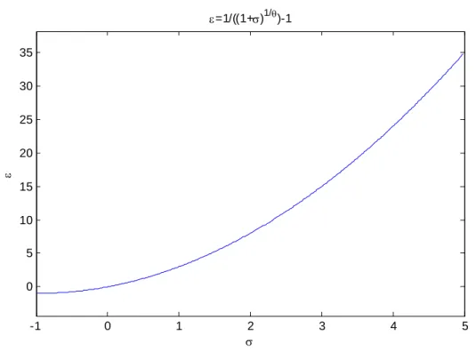
Experiment 1 observes the relation between the exogenous technology shock,i t, , and the growth rate of city size,i t, . The functions of city growth given negative local size effect,e, are shown in Figure 1.1~Figure 1.6. The city growth rate,i t, , is positively
related to the exogenous technology shock,i t, .4 Bigger technology shocks promote
4 1+
,
i t
the productivity of local firms; higher profit of the city will lead to higher city growth rate provided negative net local size effect. Moreover, the larger the influence of the negative net local size affect, the smaller the city growth rate given the same shock. Negative local externalities will hinder the growth of city.
5.2 Experiment 2: the mean of exogenous technology shock
The equilibrium size of cities at time t, , , is a function of the exogenous technology shock and the local size effect. The influence of the exogenous technology shock on city size is conditional on the net local size effect.
1/ , ( , 1(1 ,)) e i t i t i t S K A (15) 1/ 1 , / , (1/ ) , 0, 0 e i t i t i t dS d K e A if e
When the net local size effect is negative, cities with larger technology shocks will have larger cities. Bigger shocks lead to larger cities. This is consistent with the theoretical result in Eeckhout (2004).
We simulate cities growth by various assumption of the distribution of exogenous technology shock to investigate how the distribution of shocks affects the distribution of cities. In experiment 2, different values of the mean of shocks are applied in the simulations.
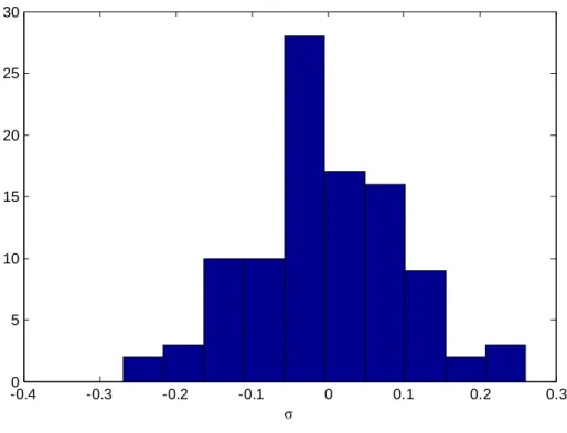
Figure 2.1~2.6 are the corresponding results given the mean of shock equals zero. Figure 2.1 is the generated normal shock distribution given zero mean. Figure 2.2 is the distribution of the derived city size growth rate, which is correlated to the distribution of exogenous technology shock. Figure 2.3 is the corresponding evolution of all cities. Figure 2.4 is the city size distribution at t=100, and Figure 2.5 is the city size distribution at t=200. It is more skew to the right as time increase. Figure 2.6 is the distribution of city size at t=200.
Figure 3.1~3.4 are the corresponding results given the mean of shock equals 0.06. Figure 3.1 is the generated normal shock distribution. Figure 3.2 is the distribution of the derived cities growth rate, which is correlated to the distribution of exogenous technology shock. Figure 3.3 is the corresponding evolution of all cities. Figure 3.4 is the city size distribution at t=200.
Figure 4.1~4.4 are the simulated results given the mean of shock equals 0.1. Figure 4.1 is the generated normal shock distribution. Figure 4.2 is the distribution of the derived cities growth rate. Figure 4.3 is the corresponding evolution of all cities. Figure 4.4 is the city size distribution at t=200 and the fitted lognormal distribution. Both
estimated parameters are significantly different from zero within 1% significant level.5 It shows that an increase in the mean of shocks will move the distribution of city growth rate to the right which accelerates the city growth; the inequality of cities is increased. This simulated result confirms the theoretical result in Eeckhout (2004). A random productivity process and local size effect could generate lognormal distributed cities. 5.3 Experiment 3: the standard deviations of exogenous technology shock
We simulate cities growth by varying the value of the standard deviations of the distribution of exogenous technology shock. Given all the other parameters the same as in simulations of Figure 3(the standard deviation of shock is 0.1), we decrease the standard deviation of shock to 0.01.
Figure 5.1~5.4 are simulated results given the standard deviation of shock equals 0.01. Figure 5.1 is the generated normal shock distribution. Figure 5.2 is the distribution of the derived cities growth rate. Figure 5.3 is the corresponding evolution of all cities. Figure 5.4 is the city size distribution at t=200 and the fitted lognormal and normal distributions.
Figure 6.1~6.4 are the results given the standard deviation of shock equals 0.001. Figure 6.1 is the generated normal shock distribution. Figure 6.2 is the distribution of the derived cities growth rate. Figure 6.3 is the corresponding evolution of all cities. Figure 6.4 is the city size distribution at t=200 and the fitted lognormal and normal distributions. Comparing to Figure 3, this experiment shows that, as the less the shocks deviates, the less the city growth rate deviates; consequently, city size are more equally distributed and the generated cities size distribution is less skew to the right.
5.4 Experiment 4: uniform distribution of exogenous technology shock
In this experiment, city size is simulated given the same parameter values as in Figure 3 except that the distribution of shock is assumed to be uniform rather than normal distribution as in Figure 3.
Figure 7.1~7.3 are the corresponding results based on the uniform distribution assumption. Figure 7.1 is the generated shock distribution. Figure 7.2 is the distribution of the derived cities growth rate which is influenced by the distribution of shock. Figure 7.3 is the corresponding evolution of all cities. The model of local externalities with random productivity process in Eeckhout (2004) could generate lognormal distributed cities conditional on the features of the distribution of the exogenous technology shock. 5.5 Experiment 5: Gini
The features of cities size distribution is determined by both the exogenous
technology shock,i t, , and the local size effect,θ. In this experiment, we investigate how exogenous technology shock and the local size effect affect the level of concentration of cities. The Gini coefficient is applied to explain the level of concentration of city size. We simulate the cities growth and fit the resulting size distribution. From Cowell (1995), Gini index = 2Φ(δ/√2) – 1, where Φ(x) is the standard normal distribution with Φ(x) = Prob(X < x). The range of the Gini coefficient is between 0 (complete equality) and 1 (complete inequality). The greater the Gini coefficient is, the more concentration of cities size. The simulated results are in Figure 8.
Figure 8.1 shows the relation between the local size effect θ and the corresponding estimated Gini coefficient with 95% confidence interval given that shocks are generated from a uniform distribution. It shows that the Gini coefficient is increasing as the absolute value of local size effect θ is decreasing. The less the absolute values of the negative local size effect, the more concentrate the cities size. The less the influence of negative local size effect, the more concentrates the city population.
Figure 8.2 shows the relation between the local size effect θ and the corresponding estimated Gini coefficient with 95% confidence interval given that shocks are generated from normal distribution with =0.5; the other condition are the same as in Figure 8.1 . Similarly to the result in Figure 8.1, the Gini coefficient is increasing as the absolute value of local size effect θ is decreasing. The less the influence of the negative local size effect, the more concentrates the cities’ population.
Figure 8.3 shows the relation between the local size effect θ and the corresponding estimated Gini coefficient with 95% confidence interval given that the shocks are generated from normal distribution with a smaller standard deviation =0.3. Similarly to the previous results, the Gini coefficient is increasing as the absolute value of local size effect θ is decreasing. Comparing to Figure 8.2, the standard deviation of exogenous technology shock is smaller. The change of the standard deviation of exogenous technology shock does not affect the sign of their relation.
Figure 8.2~8.3 shows that greater influence of the negative local externalities will decentralize cities’ population.
Figure 8.4 shows the relation between the standard deviation of exogenous technology shock and the corresponding estimated Gini coefficient with 95% confidence interval given =-1.1. The Gini coefficient is increasing as the standard deviation of shock is increasing. The more the exogenous technology shock deviated, the more concentrate cities population. The less the technology shock deviated; the more decentralized the city population.
Figure 8.5 is the relation between the estimated Gini coefficient with 95% confidence interval and the standard deviation of exogenous technology shock given = -2. Comparing to Figure 8.5, a change in the net local size effect does not change the positive relation between Gini and the standard deviation of exogenous technology shock . The relation of the level of concentration of cities population and the deviation of shock is not sensitive to the change of the net local size effect.
Figure 8.6 shows the relation between the estimated Gini coefficient with 95% confidence interval and the mean of exogenous technology shock . We do not see a systematic relation between mean of exogenous technology shock and the level of concentration of cities population.
6 Congestion cost and the level of concentration
The size elasticity of production, parameter e in equation (4), is composed of the positive local externalities as knowledge spillover and the negative local externalities as congestion and transport cost. It is a net effect of positive and negative externalities. In the theory, the size elasticity of production is crucial in determining motion and resulting size distribution of cities. Change of congestion cost affects the growth process of cities, and consequently the size distribution of cities.
We simulate the growth of city population based on the model in Eeckhout (2004) to examine the relation between the size elasticity of production and the resulted city sizes distribution. The equilibrium city size is determined by city-specific technology shock and local externalities. In the simulation, technology shock and positive local externalities are exogenous. The technology shock is symmetric and identically independently distributed. The equilibrium city sizes and the growth of cities are endogenously determined in the model given various negative local externality denoted as transport cost in the size elasticity of production
Further, the Gini coefficient is applied to measure concentration of population across cities. The growths of size of cities are simulated and the corresponding Gini coefficient of the resulting size distribution of cities is estimated.6
The simulated result is in Figure 9. Larger value of the Gini coefficient represents more concentrate among cities; on the contrary, smaller value of Gini denotes a more evenly distributed cities population across cities. The size of cities is identical if the Gini coefficient is 0, and the size of cities is perfectly unequal if the Gini coefficient is 1. Figure 1 shows the relation between congestion cost and the corresponding estimated Gini coefficient. The trend in figure shows that the larger the congestion cost, the
6 Gini index = 2Φ(δ/√2) – 1, where Φ(x) is the standard normal distribution with Φ(x) = Prob(X < x).
smaller the estimated Gini. An increase of congestion cost may lead to more evenly distributed cities population; on the other hand, a decrease of congestion cost increases the advantage of agglomeration which may raise the size of large cities in the region; the degree of inequality of city size will increase.
7 Conclusion
In this paper, the relation between the exogenous technology shock, and the growth rate of city size, conditional on the local size effect, is investigated. Growth of cities is simulated given various parameter of the distribution of exogenous technology shock to investigate how the distribution of shocks affects the distribution of cities. Cities growth is simulated given different value of the standard deviations or the mean of the exogenous technology shock; moreover, cities growth is simulated given different assumption distribution. Finally, we investigate how exogenous technology shock and the local size effect affect the level of concentration of cities. The Gini coefficient is applied to explain the level of concentration of cities size. The relation is investigated by various assumption of distribution, the values of mean and standard deviation of exogenous technology shock, and local size effect.
The simulation result shows that the city growth rate is positively related to the exogenous technology shock, given negative net local size effect. This is consistent with the theoretical result in Eeckhout (2004). The greater the exogenous technology shock, the greater the city growth rate. Bigger technology shocks promote the productivity of local firms, and lead to higher city growth rate provided negative net local size effect. The larger the absolute value of the net local size effect, the smaller the city growth rate. Smaller influence of the negative net local size effect will accelerate city growth rate. Negative local externalities will hinder the growth of city.
An increase in the mean of shocks will increase city growth rate, and subsequently the inequality of cities is increased. The less the shocks deviates, the less the city growth rate deviates; consequently, city size are more equally distributed and the generated cities size distribution is less skew to the right. The distribution of shocks affects the distribution of city growth rate and city size. Uniformly distributed shocks will lead to more evenly distributed cities. The model of local externalities with random productivity process in Eeckhout (2004) could generate lognormal distributed cities conditional on the features of the distribution of the exogenous technology shock.
The Gini coefficient is increasing as the absolute value of local size effect is decreasing. The less the influence of the negative local size effect, the more concentrates the city size. Bigger influence of the negative local externalities will decentralize cities’ population. The Gini coefficient is increasing as the standard deviation of exogenous technology shock is increasing. The more the exogenous
technology shock deviated, the more city size concentrates. The less the technology shock deviated; the more decentralized the city population.
A change in the net local size effect does not change the positive relation between Gini and the standard deviation of exogenous technology shock. The relation of the level of concentration of cities population and the deviation of shock is not sensitive to the change of the net local size effect. We do not see a systematic relation between the mean of exogenous technology shock and the level of concentration of cities population. Smaller negative local externalities or more diverge technology shock could generate bigger cities. We also finds that the theory implies that larger shocks lead to larger cities when the size elasticity of production is negative; larger productivity shocks lead to bigger cities if the congesting cost dominates the net local externalities. Moreover, an increase of congestion cost will lead to more evenly distributed cities.
Reference
Bee, Riccaboni, and Schiavo (2013), The size distribution of US cities: Not Pareto, even in the tail, Economics Letters, 120(2), 232–237.
Berry, B.J. L., and A. Okulicz-Kozaryn (2012), The city size distribution debate: Resolution for US urban regions and megalopolitan areas, Cities 29, (Suppl. 1) S17– S23.
Blank, Aharon and Solomon, Sorin (2000), Power Laws in Cities’ Population, Financial Markets and Internet Sites (Scaling in Systems with a Variable Number of Components). Physica A, 287(1–2), pp. 279–88.
Cowell, F. (1995): Measuring Inequality, LSE Handbooks on Economics Series. Prentice Hall, London.
Eeckhout, J. (2004). Gibrat’s law for (all) cities. American Economic Review, 94 (5), 1429–1451.
Eeckhout, J. (2009). "Gibrat's Law for (All) Cities: Reply." American Economic Review, 99(4): 1676-83.
Ioannides Y. and Skouras S. (2013), US city size distribution: Robustly Pareto, but only in the tail, Journal of Urban Economics,Volume 73, Issue 1, January 2013, Pages 18–29.
Lee, and Q. Li, (2013), Uneven landscapes and city size distributions, Journal of Urban Economics, 78, 19-29.
Levy, Moshe (2009). ‘Gibrat’s law for (all) cities: comment. American Economic Review, 99 (4), 1672–1675.
Lucas, Robert E., Jr. and Rossi-Hansberg, Esteban, (2002), The Internal Structure of Cities. Econometrica, 70(4), pp. 1445–76.
Malevergne, Y., Pisarenko, V. and Sornette, D. (2011), Testing the Pareto against the lognormal distributions with the uniformly most powerful unbiased test applied to the distribution of cities, Physical Review E 83, 036111(11)
Gabaix, X. (1999a), Zipf’s Law for Cities: An Explanation, Quarterly Journal of Economics, 114 (3), 739–767.
Gabaix, X. (1999b), Zipf’s Law and the Growth of Cities, American Economic Review Papers and Proceedings, 89 (2), 129–132.
Gibrat R. ,(1931), “Les inegalites economiques”, Paris: Librairie du Recueil Sirey. Rossi-Hansberg, Esteban and Mark L. J. Wright, 2007, Urban structure and growth. Review of Economic Studies 74(2):597–624.
Rybski, Diego, Anselmo García Cantú Ros, and Jürgen P. Kropp, 2013, "Distance-weighted city growth." Physical Review E 87.4: 042114.
Veneri (2013), On City Size Distribution, Evidence from OECD Functional Urban Areas, American Economic Review, 94(5): 1429-1451.
Fig. 1.1 The relation between the exogenous technology shock,i t, , and the growth
rate of city size,i t, , given the local size effect = ‐0.1.
Fig. 1.2 The relation between the exogenous technology shock,i t, , and the growth
rate of city size,i t, , given the local size effect = -0.5.
-1 0 1 2 3 4 5 0 0.5 1 1.5 2 2.5 3 x 107 =1/((1+)1/)-1 -1 0 1 2 3 4 5 0 5 10 15 20 25 30 35 =1/((1+)1/)-1
Fig. 1.3 The relation between the exogenous technology shock,i t, , and the growth
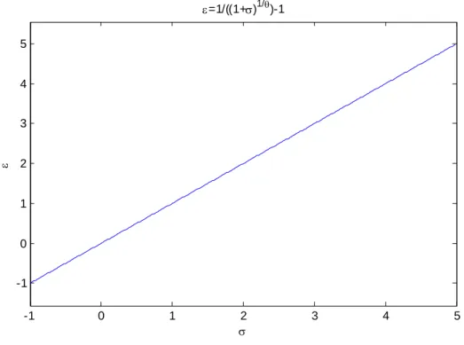
rate of city size,i t, , given the local size effect = -1.
Fig. 1.4 The relation between the exogenous technology shock,i t, , and the growth
rate of city size,i t, , given the local size effect = -1.5.
-1 0 1 2 3 4 5 -1 0 1 2 3 4 5 =1/((1+)1/)-1 -1 0 1 2 3 4 5 6 -1 -0.5 0 0.5 1 1.5 2 2.5 3 =1/((1+)1/)-1, = -1.5
Fig. 1.5 The relation between the exogenous technology shock,i t, , and the growth
rate of city size,i t, , given the local size effect = -2.
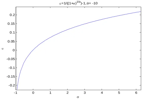
Fig. 1.6 The relation between the exogenous technology shock,i t, , and the growth
rate of city size,i t, , given the local size effect = -10.
-1 0 1 2 3 4 5 6 -1 -0.5 0 0.5 1 1.5 =1/((1+)1/)-1, = -2 -1 0 1 2 3 4 5 6 -0.2 -0.15 -0.1 -0.05 0 0.05 0.1 0.15 0.2 =1/((1+)1/)-1, = -10
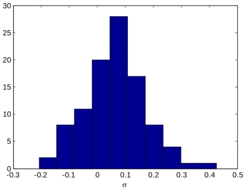
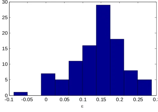
Fig. 2.1 The distribution of the exogenous technology shock,i t, , given its mean = 0.
Fig. 2.2 The distribution of the growth rate of city size,i t, , given the mean of the
distribution of the exogenous technology shock,i t, equals 0.
-0.40 -0.3 -0.2 -0.1 0 0.1 0.2 0.3 5 10 15 20 25 30 -0.250 -0.2 -0.15 -0.1 -0.05 0 0.05 0.1 0.15 0.2 5 10 15 20 25
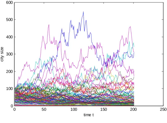
Fig. 2.3 The evolution of city size,S , given the mean of the distribution of the i t,
exogenous technology shock,i t, equals 0.
Fig. 2.4 The distribution of city size at t=100 given the mean of the distribution of the exogenous technology shock,i t, equals 0.
0 50 100 150 200 250 0 100 200 300 400 500 600 time t ci ty s iz e 0 50 100 150 200 250 300 350 400 450 500 0 10 20 30 40 50 60 70 city size at t/2
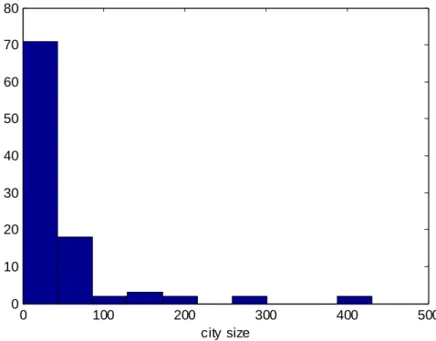
Fig. 2.5 The distribution of city size at t=200 given the mean of the distribution of the exogenous technology shock,i t, equals 0.
Fig. 2.6 The fitted lognormal distribution of city size at t=200 given the mean of the distribution of the exogenous technology shock,i t, equals 0.
0 100 200 300 400 500 0 10 20 30 40 50 60 70 80 city size 0 50 100 150 200 250 300 350 400 0 0.005 0.01 0.015 0.02 0.025 0.03 0.035 0.04 0.045 Size De nsi ty data Lognormal
Fig. 3.1 The distribution of the exogenous technology shock,i t, , given its mean =
0.06.
Fig. 3.2 The distribution of the growth rate of city size,i t, , given the mean of the
distribution of the exogenous technology shock,i t, equals 0.06.
-0.30 -0.2 -0.1 0 0.1 0.2 0.3 0.4 0.5 5 10 15 20 25 30 -0.20 -0.1 0 0.1 0.2 0.3 5 10 15 20 25 30
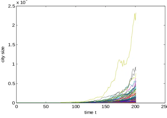
Fig. 3.3 The evolution of city size,S , given the mean of the distribution of the i t,
exogenous technology shock,i t, equals 0.06.
Fig. 3.4 The distribution of city size at t=200 given the mean of the distribution of the exogenous technology shock,i t, equals 0.06.
0 50 100 150 200 250 0 0.5 1 1.5 2 2.5x 10 6 time t ci ty si ze 0 5 10 15 x 105 0 10 20 30 40 50 60 70 city size
Fig. 4.1 The distribution of the exogenous technology shock,i t, , given its mean =
0.2.
Fig. 4.2 The distribution of the growth rate of city size,i t, , given the mean of the
distribution of the exogenous technology shock,i t, equals 0.2.
-0.20 -0.1 0 0.1 0.2 0.3 0.4 0.5 5 10 15 20 25 30 -0.10 -0.05 0 0.05 0.1 0.15 0.2 0.25 0.3 5 10 15 20 25 30
Fig. 4.3 The evolution of city size,S , given the mean of the distribution of the i t,
exogenous technology shock,i t, equals 0.2.
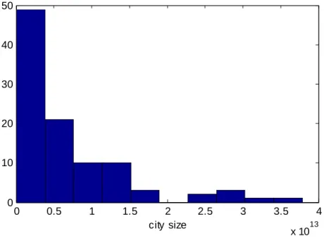
Fig. 4.4 The distribution of city size at t=200 given the mean of the distribution of the exogenous technology shock,i t, , equals 0.2.
0 50 100 150 200 250 0 0.5 1 1.5 2 2.5 3 3.5 4 4.5x 10 13 time t ci ty si ze 0 0.5 1 1.5 2 2.5 3 3.5 4 x 10¹³ 0 10 20 30 40 50 city size
Fig. 5.1 The distribution of the exogenous technology shock,i t, , given its standard
deviation = 0.01.
Fig. 5.2 The distribution of the growth rate of city size,i t, , given the standard
deviation of the distribution of the exogenous technology shock,i t, equals 0.01.
0.020 0.03 0.04 0.05 0.06 0.07 0.08 5 10 15 20 25 0.010 0.02 0.03 0.04 0.05 0.06 5 10 15 20 25
Fig. 5.3 The evolution of city size,S , given the standard deviation of the distribution i t,
of the exogenous technology shock,i t,,equals 0.01.
Fig. 5.4 The distributions of city size at t=200 given the standard deviation of the distribution of the exogenous technology shock,i t, ,equals 0.01.
0 50 100 150 200 250 0 0.5 1 1.5 2 2.5 3 3.5 4 4.5x 10 5 time t ci ty s iz e 0 0.5 1 1.5 2 2.5 3 3.5 4 x 10⁵ 0 2 4 6 8 10 12 14 16 city size
Fig. 6.1 The distribution of the exogenous technology shock,i t, , given its standard
deviation = 0.001
Fig. 6.2 The distribution of the growth rate of city size,i t, , given the standard
deviation of the distribution of the exogenous technology shock,i t, ,equals 0.001.
0.0560 0.057 0.058 0.059 0.06 0.061 0.062 0.063 5 10 15 20 0.04 0.0405 0.041 0.0415 0.042 0.0425 0.043 0.0435 0.044 0.04450 2 4 6 8 10 12 14 16 18 20
Fig. 6.3 The evolution of city size,S , given the standard deviation of the distribution i t,
of the exogenous technology shock,i t,,equals 0.001.
Fig. 6.4 The distribution of city size at t=200 given the standard deviation of the distribution of the exogenous technology shock,i t, , equals 0.001.
0 50 100 150 200 250 0 0.5 1 1.5 2 2.5 3 3.5 4 4.5x 10 5 time t ci ty s iz e 0 0.5 1 1.5 2 2.5 3 3.5 4 x 10⁵ 0 2 4 6 8 10 12 14 city size
Fig. 7.1 The generated random distribution of the exogenous technology shock,i t, ,
given uniform distribution assumption.
Fig. 7.2 The distribution of the growth rate of city size,i t, , given uniform distribution
of the exogenous technology shock,i t, .
0 0.2 0.4 0.6 0.8 1 0 5 10 15 0 0.1 0.2 0.3 0.4 0.5 0.6 0.7 0 2 4 6 8 10 12 14 16 18
Fig.7.3 The evolution of city size,S , given uniform distribution of the exogenous i t,
technology shock,i t, .
Fig. 8.1 The relation between the estimated Gini coefficient with 95% confidence interval and the local size effect θ given that exogenous technology shock is from uniform distribution. 0 20 40 60 80 100 120 0 2 4 6 8 10 12 14 16 18x 10 13 time t ci ty si ze -2.5 -2 -1.5 -1 -0.5 0 0.5 0.6 0.7 0.8 0.9 1 Gi n i Gini GiniCI GiniCI
Fig. 8.2 The relation between the estimated Gini coefficient with 95% confidence interval and the local size effect θ given that exogenous technology shock is from normal distribution with =0.5.
Fig. 8.3 The relation between the estimated Gini coefficient with 95% confidence interval and the local size effect θ given exogenous technology shock is from normal distribution with =0.3. -2 -1.5 -1 -0.5 0.7 0.75 0.8 0.85 0.9 0.95 1 Gi n i Gini Gini CI Gini CI -2 -1.5 -1 -0.5 0.4 0.5 0.6 0.7 0.8 0.9 1 Gi n i Gini Gini CI Gini CI
Fig. 8.4 The relation between the estimated Gini coefficient with 95% confidence interval and the standard deviation of exogenous technology shock given θ =-1.1.
Fig. 8.5 The relation between the estimated Gini coefficient with 95% confidence interval and the standard deviation of exogenous technology shock given θ = -2.
0.1 0.15 0.2 0.25 0.3 0.35 0.4 0.45 0.5 0.5 0.55 0.6 0.65 0.7 0.75 0.8 0.85 0.9 0.95 1 Gi n i Gini Gini CI Gini CI 0.1 0.15 0.2 0.25 0.3 0.35 0.4 0.45 0.5 0.4 0.45 0.5 0.55 0.6 0.65 0.7 0.75 0.8 0.85 0.9 Gi n i Gini Gini CI Gini CI
Fig. 8.6 The relation between the estimated Gini coefficient with 95% confidence interval and the mean of exogenous technology shock .
Fig. 9. Congestion cost and the estimated Gini coefficient with 95% confidence interval 0 0.5 1 1.5 0.54 0.56 0.58 0.6 0.62 0.64 0.66 0.68 0.7 0.72 0.74 Gi n i 0.5 1 1.5 2 2.5 3 0.4 0.5 0.6 0.7 0.8 0.9 1 Congestion cost Gi n i
104年度專題研究計畫成果彙整表
計畫主持人:陳心蘋 計畫編號:104-2410-H-004-200-計畫名稱:外部經濟與都市分佈 成果項目 量化 單位 質化 (說明:各成果項目請附佐證資料或細 項說明,如期刊名稱、年份、卷期、起 訖頁數、證號...等) 國 內 學術性論文 期刊論文 1 篇 陳心蘋, 2015年, “An Analysis of the Form of Local Externality”, 建 築與規劃學報, 16卷2&3期, p.151 – 161. (ACI ,Scopus) 研討會論文 0 專書 0 本 專書論文 0 章 技術報告 0 篇 其他 0 篇 智慧財產權 及成果 專利權 發明專利 申請中 0 件 已獲得 0 新型/設計專利 0 商標權 0 營業秘密 0 積體電路電路布局權 0 著作權 0 品種權 0 其他 0 技術移轉 件數 0 件 收入 0 千元 國 外 學術性論文 期刊論文 0 篇 研討會論文 0 專書 0 本 專書論文 0 章 技術報告 0 篇 其他 0 篇 智慧財產權 及成果 專利權 發明專利 申請中 0 件 已獲得 0 新型/設計專利 0 商標權 0 營業秘密 0 積體電路電路布局權 0著作權 0 品種權 0 其他 0 技術移轉 件數 0 件 收入 0 千元 參 與 計 畫 人 力 本國籍 大專生 0 人次 碩士生 3 彭思瑾,郭獻聰,王靖筑 博士生 0 博士後研究員 0 專任助理 0 非本國籍 大專生 0 碩士生 0 博士生 0 博士後研究員 0 專任助理 0 其他成果 (無法以量化表達之成果如辦理學術活動 、獲得獎項、重要國際合作、研究成果國 際影響力及其他協助產業技術發展之具體 效益事項等,請以文字敘述填列。)