利用屬性分群之特徵選擇及其應用

全文

(1)國立高雄大學電機工程學系(研究所) 碩士論文. 利用屬性分群之特徵選擇及其應用 Feature Selection by Attribute Clustering and Its Applications. 研究生：劉彥良撰指導教授：洪宗貝. 中華民國九十六年八月.

(2) Feature Selection by Attribute Clustering and Its Applications Advisor: Dr.(Professor) Tzung-Pei Hong Institute of Electrical Engineering National University of Kaohsiung Student: Yan-Liang Liou Institute of Electrical Engineering National University of Kaohsiung. ABSTRACT. Feature selection is to find useful and relevant features from an original feature space to effectively represent and index a given dataset. It is very important to classification and clustering problems, which may be quite difficult to solve when the amount of attributes in a given training data is very large. After feature selection, the rules derived from only the selected features may be hard to use if some values of the selected features cannot be obtained in current environments. In this thesis, we try to select representative features by attribute clustering, and the attributes grouped together in the same clusters can aid the classification work later. Like conventional clustering for objects, the attributes within the same cluster have high similarity, and within different clusters have high dissimilarity. Three similarity measures for a pair of attributes are thus presented. Two attribute clustering algorithms based on the similarity measures are then proposed. The first one, called Most Neighbors First (MNF), clusters the attributes into a pre-defined number of groups. The second one, based on the CAST algorithm, clusters the attributes into an appropriate number of clusters even when the cluster number cannot be obtained in advance. The representative attributes found in the clusters can then be used for classification such that the whole feature space can be greatly reduced. Besides, two classification algorithms based on the proposed attribute clustering approaches are described to solve the problem that some values of the selected features cannot be obtained in current situations. One is based on case-based reasoning and the other is based on the k-nearest-neighbors classifier. By attribute clustering and attribute replacement, some other possible attributes in the same clusters can be used to achieve approximate inference results. Keywords: attribute clustering, feature space, dissimilarity measure, rough set, representative attribute. I.

(3) 利用屬性分群之特徵選擇及其應用指導教授：洪宗貝博士（教授）國立高雄大學電機工程所學生：劉彥良國立高雄大學電機工程所. 摘要. 特徵選擇是由原始特徵空間中挑選一組有用且合適的特徵以便有效地對資料作描述與索引，這項工作對處理分類及分群問題上很重要。然而，當訓練用的資料屬性量大時這卻變的十分困難。此外，當某些屬性(特徵)已被挑選出，則之後所推導出的分類規則將只會由這些屬性所構成，然而，有時我們無法在目前環境下取得這些屬性的數值，則之前推導出的分類規則將無法被利用。在這篇論文中，我們嘗試對屬性分群並從中選取代表的屬性以達到降低屬性數目，且被群組於同一群之屬性亦可輔助日後的分類工作。如同一般對個體的分群，落在同群的屬性彼此會有較高的相似度，而落在不同群的屬性則會有較高的相異度。我們提出三種量度屬性相似度的方法，以及兩個基於這些量度法的屬性分群演算法。第一個稱為最多鄰居優先法，它可依照設定的群數將屬性完成分群。第二個則是基於 CAST 演算法，它可將屬性群聚成適當的群數，即使無法事先得知屬性的群數。接著，由各群中選出代表的屬性來處理之後的分類工作。我們提出兩個基於屬性分群法的分類演算法，分別改良了基於案例的推理分類法與 k-最鄰近分類法。整體而言，利用屬性的分群結果來選擇屬性，除了可降低分類問題的複雜度，當某些被選出的屬性該數値無法得知之時，則可利用屬性取代法的技巧，以同群其他屬性達到近似的推論結果。實驗結果亦證明了所提出的方法之有效性。關鍵字：屬性分群、特徵空間、相異度量測、約略集合、代表屬性。. II.

(4) 謝誌. 呼! 這篇論文總算在最後一刻完成了。首先我要感謝指導老師洪宗貝教授，若非他慧眼獨具堅持這個想法可行，我也不會推出後面一系列的作法與應用，當然，也要感謝洪老師總是犧牲難得的休閒時間，與我討論文方向或指導論文寫作。接著我要感謝兩位口試委員，林文揚教授與黃國禎教授，感謝他們百忙之中撥冗參與我的論文口試並當場提出極具建設性的意見，使得這篇碩士論文更瑧完善。然而，由於時間緊迫有些可加強說服力的實驗數據仍未提到，在此謹向兩位老師致歉，這部份的工作會在日後發表論文中再一一補強。兩年的碩班生活好比洗芬蘭浴! 先是當了一年的實驗室宅男，幸虧有詠騏學長和其他神龍般的學長們:俊豪、Jerry、明泰和國能的出現，在此感謝他們當時給予我生活上及學術上的指引，使得我可以在短時間內適應枯燥的研究生活，並從中發掘興趣而一路走過來。再來要感謝實驗室的其他同學俊松、承熹和廷政，在修課及研究上給予的協助，使得程式功力可以大幅進步。另外，感謝陸續加入的學弟妹:阿銅、怡穎、韋体、卓翰… 等，以及其他實驗室的同學:瀞誼、明訓…等，謝謝你們為我ㄧ陳不變的研究生活增添不少光彩與樂趣。此外還有學校行政人員:系辦姿容、計中姿容，及會計室玉露、意藍… 等，感謝你們的熱心協助與指點，使得我研究助理的工作得以順利完成。當然，這篇論文的幕後推手還有我親愛的家人及默默承受無聊的惠芬，因為你們的包容與諒解，我才可以專心完成這篇論文並實現自己的理想。最後，僅向這段日子曾經幫助我、鼓勵我的所有朋友致上最深的謝意。. 劉彥良 2007,8 於 NUK III.

(5) Contents. ABSTRACT.......................................................................................................... I 摘要. ............................................................................................................. II. 謝誌. ............................................................................................................III. Contents ........................................................................................................... IV List of Figures .................................................................................................... VI List of Tables..................................................................................................... VII CHAPTER 1 Introduction.....................................................................................1 1.1 Background and Motivation ........................................................................................1 1.2 Contributions................................................................................................................4 1.3 Thesis Organization .....................................................................................................5. CHAPTER 2 Literature Survey ............................................................................6 2.1 Feature Selection..........................................................................................................6 2.2 Reducts.........................................................................................................................9 2.3 Relative Dependency .................................................................................................11 2.4 The k-means and the k-medoids Clustering Approaches ...........................................12 2.5 Clustering with Unknown Cluster Numbers..............................................................14 2.6 Case-Based Reasoning...............................................................................................16 2.7 k-Nearest-Neighbor Classifier ...................................................................................17. CHAPTER 3 Calculation of Attribute Similarity ...............................................18 3.1 Attribute Similarity Based on Relative Dependency .................................................18 3.2 Attribute Similarity Based on Majority Sets..............................................................19 IV.

(6) 3.3 Generalized Attribute Similarity Based on Majority Sets..........................................22. CHAPTER 4 Attribute Clustering with Pre-Defined Cluster Numbers .............28 4.1 The Basic Concepts of the Proposed Algorithm ........................................................28 4.2 The Proposed Algorithm ............................................................................................29 4.3 An Example................................................................................................................32 4.3 Experimental Results .................................................................................................36. CHAPTER 5 Attribute Clustering with Unknown Cluster Numbers .................40 5.1 The Basics of the Proposed Algorithm ......................................................................40 5.2 The Proposed Algorithm ............................................................................................41 5.3 An example ................................................................................................................43. CHAPTER 6 Case-Based Reasoning with Attribute Clustering ........................49 6.1 The Proposed Algorithm ............................................................................................49 6.2 Examples....................................................................................................................53. CHAPTER 7 The k-Nearest-Neighbors Classifier with Attribute Clustering ....60 7.1 The Proposed Algorithm ............................................................................................60. CHAPTER 8 Conclusions and Future Works .....................................................64 References ...........................................................................................................65. V.

(7) List of Figures. Figure 2.1: The conventional framework of the subset evaluation strategy. ........7 Figure 4.1: The average S_in along with numbers of clusters............................37 Figure 4.2: The average D_in along with numbers of clusters...........................37 Figure 4.3: The times of being selected as centers for each attribute for k=3. ...38 Figure 4.4: The times of being selected as centers for each attribute for k=6. ...38 Figure 4.5: The times of being selected as centers for each attribute for k=9. ...39 Figure 6.1: The concept of attribute clusters. .....................................................54. VI.

(8) List of Tables. Table 2.2: A simple information system. ............................................................10 Table 2.3: A simple decision system. ..................................................................10 Table 3.1: A simple decision system to evaluate the similarity. .........................19 Table 3.2: A simple information system to evaluate the dependency. ................22 Table 3.3: The transformed table of Table 3.2. ...................................................23 Table 3.4: The four cases for the dependency DepM+(Ai, Aj) .............................25 Table 4.1: A simple decision system. ..................................................................29 Table 4.2: An example for attribute clustering. ..................................................33 Table 4.3: The distances between non-center attributes and representative centers.................................................................................................34 Table 4.4: The distances between any two attributes within the same clusters..34 Table 4.5: The characteristics of the dataset, wdbc. ...........................................36 Table 5.1: An example for attribute clustering. ..................................................44 Table 5.2: The resulting majority similarity values for all pairs of attributes. ...45 Table 5.3: The affinity of each attribute..............................................................45 Table 5.4: The entire process of Steps 3 to 4. .....................................................46 Table 5.5: The updated affinity after SE is removed from Copen. ........................47 Table 5.6: The updated affinity after adding CH to Copen. ..................................47 Table 6.1: Three constructed attribute clusters. ..................................................54 Table 6.2: The case base in Example 1. ..............................................................55 Table 6.3: An object xa to be classified in Example 1.........................................55 Table 6.4: The dissimilarity between xa and each case in Example 1. ...............56 VII.

(9) Table 6.5: An object xb to be classified in Example 2.........................................57 Table 6.6: The dissimilarity between xb and each case in Example 2. ...............57 Table 6.7: Five cases in Example 3.....................................................................58 Table 6.8: The dissimilarity between xa and each case in Example 3. ...............59. VIII.

(10) CHAPTER 1 Introduction 1.1 Background and Motivation Expert systems have been widely used in domains where mathematical models cannot easily be built, human experts are not available or the cost of querying an expert is high. Although a wide variety of expert systems have been built, knowledge acquisition remains a development bottleneck. A knowledge engineer is thus usually needed to establish a dialog with a human expert and to encode the knowledge elicited into a knowledge base for producing an expert system. The process is, however, very time-consuming [7][33]. Building a large-scale expert system involves creating and extending a large knowledge base over the course of many months or years. Shortening the development time is thus the most important factor for the success of an expert system. In the past, machine-learning techniques were thus been successfully developed to ease the knowledge-acquisition bottleneck. Among the proposed approaches, deriving rules from training examples is the most common [22][28][29]. Given a set of examples, a learning program tries to induce rules that describe each class. Feature selection is a process of selecting relevant features (or removing irrelevant and redundant features) for representing data. It is a critical step in preprocessing for high-dimensional classification problems. Deriving rules for classification based on selected features can not only reduce the execution time but also make the results simple and easily interpreted. In the past, some researches considered feature selection as a search problem, in which the states in the search space represent the possible feature subsets. Finding an optimal (minimal) feature subset has, however, been shown to be NP-hard [4]. Many search strategies. 1.

(11) such as sequential forward search (SFS), sequential backward search (SBS), random search and hill climbing [16][5][11][32] were thus proposed to balance the computation complexity and the optimality of results. No matter which search strategy was used, a suitable evaluation method to measure the goodness of an individual feature or a feature subset was necessary. Some researches thus addressed on evaluation methods for selecting relevant features. They included. using. information. gain. [18],. correlation-based. subset. selection. [15],. consistency-based subset selection [1][26], random sampling incorporated with attribute weighting (i.e. relief) [21][24]. Another approach for feature selection is based on the rough set theory [30][31], which was proposed by Pawlak. In the approach, the reduced set of attributes (features) is called a “reduct” and many possible reducts may exist at the same time. A minimal reduct, just as its literal meaning shows, is a reduct which cannot be reduced any more. It may not be unique as well. The classification work for a high-dimensional dataset based on a minimal reduct can usually be processed faster than on an original entire set of attributes. Finding a minimal reduct is an NP-hard problem [33]. Some researches about finding approximate reducts were thus proposed. An approximate reduct is a minimal reduct with acceptable tolerance. It can usually be found in much shorter time than an exact minimal reduct. It is a good trade-off among accuracy, practicability and execution time. In the past, many approaches for finding approximate reducts were proposed [19][42][43]. For example, Wróblewski used the genetic algorithm to find approximate minimal reducts [39]. Sun and Xiong proposed an approach compatible with incomplete information systems [38]. Al-Radaideh et al. used the discernibility matrix and a weighting strategy to find minimal reducts in a greedy way [2]. Gao et al. proposed a feature ranking strategy (similar to attribute weighting) with a sampling process included [12]. Although the above approaches. 2.

(12) can select features or find reducts, they may not work well when training examples contain missing or unknown attribute values. Besides, if only the selected attributes are used in the learning process, the rules cannot contain other attributes and are difficult to use if some values of the selected attributes cannot be obtained in current environments. In this thesis, we solve the above problems from another viewpoint – attribute clustering. Note that we are doing clustering for attributes rather than for objects. Like the conventional clustering approaches for objects, we would like to have the attributes within the same cluster possess high similarity, but within different clusters possess low similarity. In this thesis, we use the average dependency degree to represent the similarity between two attributes. And three evaluation methods for attribute similarity are proposed. We then proposed two attribute clustering algorithms based on the similarity measures. The first one called Most Neighbors First (MNF) partition the attributes into k clusters according to the dependency between each pair of attributes. It also uses a better search strategy to find centers (representative attributes) in a dense region, instead of random search in k-medoids. The second one based on the CAST algorithm [3] can partition the attributes into adequate cluster numbers even the cluster number cannot be obtained in advance. Besides, the average similarity of each cluster can be guaranteed to be above the given threshold. When the attributes are grouped into several clusters according to their similarity degrees, an attribute selected from a cluster can thus represent the attributes within the same cluster. Then the representative attributes found in the clusters can be used for classification such that the whole feature space can be greatly reduced. Additionally, an approximate reduct could be formed from the chosen attributes gathered together. Note that the obtained result in this way is usually an approximate reduct. We then propose two classification algorithms. 3.

(13) with attribute clustering to solve the problem that some values of selected features cannot be obtained for inference. In these algorithms, the clustered attributes make it possible for any attribute to be replaced by the others in the same clusters to achieve approximate inference results. Experimental results show that the average similarity of each cluster is related to the cluster number indeed. As the cluster number increases the average similarity will converge. The proposed approach has the following three advantages. The first one is guessing a missing value of an attributes from the other attributes within the same cluster should be more accurate and faster than that from all attributes. The second one is that if an object has missing values, its class can also be decided by the other attributes within the same cluster. The third one is that the proposed approach is flexible for representing rules since each attribute in a rule can be displaced with other attributes in the same cluster.. 1.2 Contributions The contributions of this thesis are stated in this section. They include the following (1) A new point of view on feature selection by performing clustering on attributes. After partitioning the attributes into several clusters, the representative attributes found in the clusters can be used for classification such that the whole feature space can be greatly reduced. The attributes clustered can aid the classification work later, e.g., guessing a missing value. (2) To measure the similarity between a pair of attributes, three evaluation methods for attribute similarity are presented. (3) Two algorithms are proposed for partitioning attributes. The first one called Most Neighbors First (MNF), clusters the attributes into a pre-defined number of groups. The. 4.

(14) second one clusters the attributes into an appropriate number of clusters even when the cluster number cannot be obtained in advance. (4) Incorporate attribute clustering with two classification approaches: the Case-Based Reasoning and the k-Nearest-Neighbors classifier.. 1.3 Thesis Organization The remaining parts of this thesis are organized as follows. Some related researches including feature selection, reduct, relative dependency, clustering, case-based reasoning and k-nearest- neighbors classifier are reviewed in Chapter 2. The proposed evaluation methods for attribute similarity are described in Chapters 3. Two attribute clustering algorithms are proposed in Chapters 4 and 5. An algorithm incorporating case-based reasoning and attribute clustering is given in Chapter 6. An algorithm incorporating k-nearest-neighbors classifier and attribute clustering is given in Chapter 7. Some conclusions and future works are given in Chapter 8.. 5.

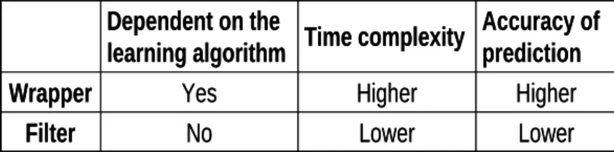
(15) CHAPTER 2 Literature Survey In this chapter, some important concepts related to this thesis are briefly reviewed. They include feature selection, reducts, relative dependency, k-means and k-medoids, some clustering approaches with unknown cluster numbers, case-based reasoning and k-nearest-neighbor classifier.. 2.1 Feature Selection In machine learning, large amount of features (attributes) will significantly slow down the learning process. The existence of redundant and irrelevant features may also cause a classifier to over-fit training data. As mentioned above, feature selection is a process of removing irrelevant and redundant features, and is popular in pattern recognition, machine learning and data mining. The approaches for feature selection can be categorized into two models, the wrapper model and the filter model. The wrapper model evaluates a set of selected features by the predictive accuracy of the learning algorithm adopted. Approaches based on the model thus depend on the learning algorithms and is computationally expensive when the number of features is large. The filter model, on the contrary, separates feature selection from classifier learning, such that it is independent of the learning algorithms. Generally speaking, the features selected by the wrapper model usually get a higher accuracy of classification than those by the filter model. A comparison of the two models is shown in Table 2.1.. 6.

(16) Table 2.1: A comparison of the wrapper and the filter models.. Dependent on the Accuracy of Time complexity learning algorithm prediction Wrapper Yes Higher Higher Filter No Lower Lower. According to feature evaluation, approaches based on feature selection can also be divided into two kinds, individual (feature) evaluation and subset evaluation [41]. The individual evaluation strategy weights (ranks) individual features according to their degrees of relevance to the decision attribute. That is, attributes are selected based on their individual importance in distinguishing the instances into different classes [5][13]. A subset of features is then found according to the ranking list. The subset evaluation strategy, on the other hand, considers a subset of attributes at the same time. It is usually composed of the following two major steps: generating candidate feature subsets and evaluating the goodness of the subsets. The conventional framework of the subset evaluation strategy is shown in Figure 2.1 [41].. Original Set. Subset Generation. Candidate Subset. Subset Evaluation Current Best Subset. No. Stopping Criterion Yes Selected Subset. Figure 2.1: The conventional framework of the subset evaluation strategy.. 7.

(17) Some approaches for evaluating the goodness of an individual feature or a subset of features have been proposed. For example, information gain was a popular ranking method used for individual attributes. It selected attributes with high differentiability to construct a decision tree. The relief approach was another individual-attribute evaluation method proposed by Kira and Rendell [21]. Its principle was that if for an attribute, the instances from different classes had different values and the ones from the same class had the same values, then the attribute was a good one for classification and should be given a high rank. The relief approach worked in a data set only with two classes (i.e. there were two possible values for the decision attribute). It proceeded in the following three main steps: (1) picking a training instance x randomly, (2) finding the nearest neighbor xP with the other class from x and updating the weight (rank) of each attribute by comparing the attribute values of x and xP, and (3) finding the nearest neighbor xS with the same class as x and updating the weight of each attribute by comparing the attribute values of x and xS. Kononenko then extended the approach to multi-class data sets [24]. Hall proposed an approach called correlation-based feature selection, which was the first one to evaluate subsets of attributes rather than individual attributes [15]. In that approach, a heuristic evaluation equation that simultaneously considered feature-class and feature-feature correlations was proposed to take the relevance and the redundancy into account. Besides, several approaches evaluated the subset of attributes by using “class consistency” [1][26]. They searched for subsets of attributes that could divide the data into groups with strong classes. Next, the concept of reducts, which is another viewpoint of feature selection, is introduced.. 8.

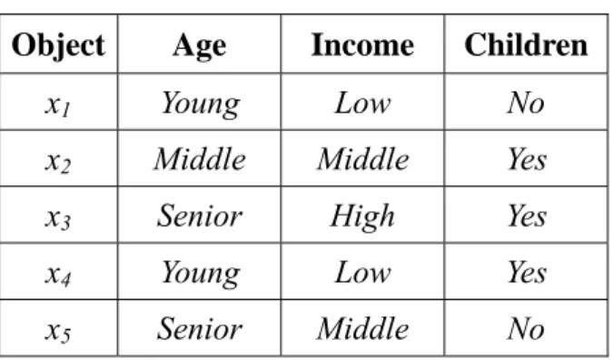
(18) 2.2 Reducts Let I = (U, A) be an information system, where U = {x1, x2, …, xN} is a finite non-empty set of objects and A is a finite non-empty set of attributes called condition attributes [23]. A decision system is an information system of the form I = (U, A∪{d}), where d is a special attribute called decision attribute and d ∉ A [23]. For any object xi ∈ U, its value for a condition attribute a ∈ A, is denoted by fa(xi). The indiscernibility relation for a subset of attributes B is defined as: IND ( B ) = {( x, y ) ∈ U × U ∀a ∈ B, f a ( x) = f a ( y )} ,. where B is any subset of the condition attribute set A (i.e. B ⊆ A) [38]. If the indiscernibility relations from both A and B are the same (i.e. IND(B) = IND(A)), then B is called a reduct of A. That means the attributes used in the information system can be reduced to B, with the original indiscernibility information still kept. Furthermore, if an attribute subset B satisfies the following condition, then B is called a minimal reduct of A:. IND( B) = IND( A) and ∀B' ⊆ B IND( B' ) ≠ IND( A). Take the simple information system in Table 2.2 as an example. In Table 2.2, the attribute set A consists of three attributes {Age, Income, Children} and the object set U consists of five objects {x1, x2, x3, x4, x5}. Since IND({Age, Children}) = IND(A) = {(x1, x1), (x2, x2), (x3, x3), (x4, x4), (x5, x5)}, the attribute subset {Age, Children} is a reduct of the information system. Besides, since neither IND({Age}) nor IND({Children}) equals IND(A), the attribute subset {Age, Children} is a minimal reduct.. 9.

(19) Table 2.2: A simple information system. Object. Age. Income. Children. x1. Young. Low. No. x2. Middle. Middle. Yes. x3. Senior. High. Yes. x4. Young. Low. Yes. x5. Senior. Middle. No. When a decision system, instead of an information system, is considered, the definition of a reduct B (B ⊆ A) can be modified as follows [39]:. ∀xi , x j ∈U , if f B ( xi ) = f B ( x j ), then d ( xi ) = d ( x j ) , where d(xi) denotes the value of the decision attribute of the object xi, fB(xi) denotes the B. attribute values of xi for the attribute set B. Similarly, if no subset of B can satisfy the above condition, B is called a minimal reduct in the decision system. Take the simple decision system shown in Table 2.3 as an example. It is modified from Table 2.2. A decision attribute, Buying Computers, is added to the original information system (Table 2.2) to form a decision system. In this example, the attribute subset {Age, Income} is not a reduct since the two objects x1 and x4 have the same values for the two attributes but belong to different classes. On the contrary, the attribute subset {Age, Children} is a reduct for the decision system. Furthermore, it is a minimal reduct since neither {Age} nor {Children} is a reduct.. Table 2.3: A simple decision system. Object. Age. x1. Young. Income Children Buying Computers. Low. No. 10. No.

(20) x2. Middle. Middle. Yes. No. x3. Senior. High. Yes. Yes. x4. Young. Low. Yes. Yes. x5. Senior. Middle. No. No. Finding minimal reducts has been proven as an NP-Hard problem. Li et al proposed the concept of “approximate” reducts [25] to speed up the searching process. An approximate reduct allows for some reasonable tolerance degrees, but can greatly reduce the computation complexity. Next, the concept of relative dependency is introduced.. 2.3 Relative Dependency Han et al. [17] and Li et al. [25] developed an approach based on the relative dependency to find approximate reducts. The relative dependency is motivated by the operation “projection”, which is very important in the relational algebra. It can also be easily executed by SQL or other query languages. Given an attribute subset B ⊆ A and a decision attribute d, the projection of the object set U on B is denoted by ΠB (U) and can be computed by the following two steps: removing attributes in the different set (A－B) and merging all the remaining rows which are indiscernible [25]. Thus, among the tuples with the same attribute values for B, only one is kept and the others are removed. For example, the projection of the data in Table 2.2 on the attribute {age} is shown below: Π{Age} (U ) = {x1, x2, x3}. In this example, x4 and x5 are removed since they have the same value of the attribute Age as x1 and x3 have. Similarly, the projection on the attribute Children and on the attribute subset {Age, Children} is shown below: 11.

(21) Π{Children} (U ) = {x1, x2}, and Π{Age, Children} (U ) = {x1, x2, x3, x4, x5}. Han et al. thus defined the relative dependency degree ( δ BD ) of the attribute subset B with regard to the set of decision attributes D as follows:. δ BD =. Π B (U ). Π B ∪ D (U ). ,. where |ΠB(U)| and |ΠB∪D(U)| are the numbers of tuples after the projection operations are performed on U according to B and B∪D, respectively. Take the decision system shown in Table 2.2 as an example. |Π{Age} (U )| = |{x1, x2, x3}| = 3 and |Π{Age, Buying Computers} (U)| = |{x1, x2, x3, x4, x3}| = 5. The relative dependency degree of {Age} with regard to {Buying Computers} is thus 3/5, which is 0.6.. 2.4 The k-means and the k-medoids Clustering Approaches The k-means and the k-medoids approaches are two well-known partitioning (or clustering) strategies. They are widely used to cluster data when the number of clusters is given in advance. The k-means clustering approach [27][18] consists of two major steps: (1) reassigning objects to clusters and (2) updating the centers of clusters. The first step calculates the distances between each object and the k centers and reassigns the object to the group with the nearest center. The second step then calculates the new means of the k groups just updated and uses them as the new centers. These two steps are then iteratively executed. 12.

(22) until the clusters no longer change. The k-medoids approach [20] adopts a quite different way of finding the centers of clusters. Assume k centers have been found. The k-medoids approach selects another object at random and replaces one of the original centers with the new object if better clustering results can be obtained. The absolute-error criterion [18] shown below is used to decide whether the replacement is better or not: k. E = ∑ ∑ p −oj , j =1 p∈C j. where E is the sum of the absolute errors for all the objects in the data set, p is an object in cluster Cj, oj is the current center of Cj, and the absolute value | p－oj | means the distance between the two objects p and oj. For each randomly selected object oj’, one of the original k centers, say oj, will be replaced with it and its new sum E’ of absolute errors will be calculated. E’ will then be compared with the previous E. If E’ is less than E, then oj’ is more suitable as a center than oj. oj’ thus actually replaces oj as a new cluster center; otherwise, the replacement is aborted. The same procedure is repeated until the cluster centers no longer change. The complexity of the k-medoids approach is in general higher than the k-means approach, but the former can guarantee that all the centers of clusters obtained are objects themselves. This feature is important to the proposed attribute clustering here since not only the attributes are clustered but also the representative attribute of each cluster has to be found. On the contrary, the k-means approach may use non-object points as cluster centers. Note that both the k-means and the k-medoids approaches are mainly designed to cluster objects, but not attributes. As mentioned above, the goal of the paper is to cluster attributes. An attribute clustering method based on k-medoids is thus proposed to achieve this purpose. It also uses a. 13.

(23) better search strategy to find centers in a dense region, instead of random selection in k-medoids. Besides, a method to measure the distances (dissimilarities) among attributes is also needed.. 2.5 Clustering with Unknown Cluster Numbers k-means and k-medoids are two well-known partitioning (or clustering) methods. They are widely used to cluster data when the number of clusters is given in advance. In real situations, it is sometimes hard to get the desired number of clusters in advance. In the past decades, many clustering approaches for this problem have been proposed. These approaches can be divided into two main classes. The first one is to design a procedure to determine the cluster number first [6][35]. Another procedure is then designed for forming the clusters according to the clustering number obtained. The kind of approaches may, however, overestimate or underestimate the cluster number, thus causing the final clustering results not completely meet users’ requirements. On the contrary, the second one is to develop new algorithms that perform clustering without deciding the desired cluster numbers in advance. For example, some approaches based on evolutionary computation have been proposed. Sarkar et al proposed a clustering approach for unknown cluster numbers based on the evolutionary programming technique [34]; Cole proposed the Genetic Clustering Algorithm (GCA) to partition objects into an adequate number of clusters [10]. Besides, some algorithms based on Artificial Neural Networks (ANN) have been proposed as well. For example, Xu et al proposed a modified competitive learning algorithm called Rival Penalized Competitive Learning (RPCL) [40]. In that algorithm, not only the weights of a winner node were modified but also the weights of the second winner (rival). 14.

(24) were considered. RPCL can automatically select an appropriate cluster number, but its performance is quite sensitive to the “de-learning” rate caused by the rival. To avoid this problem, Cheung proposed the k*-means clustering algorithm that the idea “rival” is replaced with some adjustment mechanism [9]. A particular viewpoint for clustering originated from the corrupted clique problem in the graph theory. A clique is a graph with its each vertex connected to all the other vertices; a clique graph is a graph that each connected component is a clique. The corrupted clique problem is stated as follows. Given a graph G, the problem is to find the smallest number of addition and removal of edges that will transform G into a clique graph. For clustering, the vertices in a graph represent the objects to be clustered, and two vertices are connected by an edge if their similarity is greater than or equal to a given threshold. Ben-Dor et al proposed an algorithm named Clustering Affinity Search Techniques (CAST) to perform clustering for gene expression patterns [3]. It first computed the similarity between each pair of objects and then used the similarity to partition all objects into an appropriate number of clusters under a given threshold of affinity. It used two major operations: ADD and REMOVE. The ADD operation added highly similar objects to a cluster (i.e. similarity being greater than or equal to γ); The REMOVE operation removed less similar objects from a cluster (i.e. similarity being less than γ). With these two operations, each object was then processed one by one until all objects had been assigned to clusters. The desired clusters could thus be constructed. The average similarity of the attribute pairs in the same cluster can be guaranteed to be above γ. This is the major difference between CAST and other cluster algorithms.. 15.

(25) 2.6 Case-Based Reasoning Case-Based Reasoning (CBR) is the process of solving new problems based on the solutions of similar past problems. The major tasks of CBR can be divided into five phases. When a new problem arrives, the situation of this problem is identified in the Case Representation phase. After that, the important features of the new case are extracted as its indexes in the Indexing phase. These indexes are then passed to the Matching phase for retrieving similar cases in the case base. The Adaptation phase then adapts the solutions of similar cases by adaptation rules to fit the new problem. After the final solution of the new case is confirmed by users, it is stored in the case base via the Storage phase. The success of a CBR system mainly depends on effective and efficient retrieval of similar cases for a new problem. Indexing and matching are thus very important to CBR [36]. Indexing usually uses some features of cases for identification and matching uses a pre-defined matching function for case retrieval. Each feature is given a weight to represent its importance. Based on weighted sums of features matched, similar cases in a case base can then be retrieved [8][14]. Several useful approaches have been proposed to retrieve similar cases. Two methods for assigning the weights of features were proposed by Cercone et al. [8] and Shin et al. [36]. Gupta discussed that the weights of features were different between a new case and prior cases [14]. The performance of retrieving similar cases has, however, seldom been discussed. Retrieving similar cases needs much computation time when a matching function becomes complex or when the number of cases in a case base grows large. Retrieving similar cases efficiently thus becomes an important issue in large-scale CBR.. 16.

(26) 2.7 k-Nearest-Neighbor Classifier The k-nearest-neighbor classifier (k-NN) is a method for classifying objects based on the k closest training examples in the feature space. To classify an unknown object, a k-nearest-neighbor classifier searches the feature space for the k objects that are closest to the unknown object, i.e. the k “nearest neighbor”. Then the unknown object can be classified into the major class of its k nearest neighbors. Basically, this approach is quite labor intensive, especially given a great amount of training sets or a high-dimensional feature space. That is why it proposed in the early 1950s [18], but popular until the 1960s. As the computing power has been improved, it has been widely used in the area of pattern recognition. Since the complexity of k-NN is sensitive to the size of training data and the dimension of the feature space, many approaches to speed up classification have been proposed over the years. For example: seeking to reduce the times of distance evaluations actually performed, partitioning the feature space and restricting the distance computation within specific area, and using the parallel computation technique.. 17.

(27) CHAPTER 3 Calculation of Attribute Similarity The goal of the thesis is to cluster attributes such that the efficiency of classification can be improved. For achieving this goal, it is thus important to develop an evaluation method which can measure the similarity of attributes. In this thesis, we use the dependency degree to represent the similarity between two attributes. If two attributes have high dependency degree on each other, they can be thought of as high similarity. In this chapter three evaluation methods for attribute similarity are proposed.. 3.1 Attribute Similarity Based on Relative Dependency As mentioned above, Han et al. developed an approach based on the relative dependency for finding approximate reducts [17]. We extend this metric to measure the similarity between any two attributes [25]. Given two attributes Ai and Aj, the relative dependency degree of Ai with regard to Aj was denoted by Dep(Ai, Aj) and was defined as: Dep( Ai , Aj ) =. where Π. Ai. Π Ai (U ). Π Ai , A j (U ). ,. (U ) was the projection of U on attribute Ai. Note that the original relative. dependency degree only considers the relative dependency between a condition attribute set and a decision attribute set. Here we extend the above formula to estimate the relative data dependency between any pair of attributes. The dependency degree was not symmetric, such that the condition Dep(Ai, Aj)＝Dep(Aj, Ai) was not always valid. The average of Dep(Ai, Aj). 18.

(28) and Dep(Aj, Ai) was thus used to represent the similarity of the two attributes Ai and Aj, that is: Sim( Ai , Aj ) =. Dep( Ai , Aj ) + Dep( Ai , Aj ) 2. .. 3.2 Attribute Similarity Based on Majority Sets In last section, we propose an evaluation method for attribute similarity based on relative dependency. This measure can not, however, reflect the actual similarity (dependency) of attributes in some situations. The small decision system shown in Table 3.1 is used as an example to illustrate the problem.. Table 3.1: A simple decision system to evaluate the similarity. Object. Age. Income Children Buying Computers. x1. Young. Low. No. No. x2. Young. Low. No. No. x3. Young. Low. No. Yes. x4. Young. Low. No. Yes. x5. Young. Middle. No. No. x6. Young. Middle. No. Yes. x7. Young. Middle. No. Yes. x8. Young. Middle. Yes. No. It can be observed from Table 3.1 that |Π{Age}(U)| = 1, |Π{Children}(U)| = 2 and |Π (U)| = 2. The relative dependency degrees are thus found as follows: Dep(Age, Children). {Income}. = 0.5, Dep(Age, Income) = 0.5, Dep(Children, Age) = 1, and Dep(Income, Age) = 1. Both of 19.

(29) Sim(Age, Children) and Sim(Age, Income) can then be calculated as 0.75, such that the degree for the attribute Age to resemble the attribute Children is equal to the degree for Age to resemble Income. However, it is easy to observe from Table 3.1 that Age is more similar to Children than to Income. The main reason for causing this phenomenon is due to the projection operation, which merely concerns how many distinct values exist instead of analyzing the permutation of the values. Below, another measure is proposed for evaluating the similarity of attributes more precisely. Let Ai denote the i-th attribute in an information or decision system, Vi denote the set of attribute values for attribute Ai, and vit be the t-th possible value of Ai, vit ∈ Vi. Also let X(vit) represent the set of objects whose values for attribute Ai are vit, X (vit ∧ v jt ) represent the set of objects whose values for the two attributes Ai and Aj are vit and vjs, i ≠ j. Besides, an attribute Aj is said to functionally depend on another attribute Ai (i.e., Ai → A j ) if for any vit, all the objects in X(vit) must have the same value of attribute Aj. Even if an attribute does not functionally depend on another attribute, their dependency degree may also be analyzed. Here, the dependency degree is calculated based on the idea of keeping the most objects (or removing the least objects) to make the property of functional dependency valid. According to this idea, the majority set is defined below to achieve this purpose. Let Maj Aj (vit ) be the majority set for Ai being vit on Aj, which is defined as follows:. (. ). ⎧ ⎫ Maj Aj (vit ) = ⎨v js v js ∈ V j , X (v js ∧ vit ) = max X (v jr ∧ vit ) ⎬ . r =1,",|V j | ⎩ ⎭. Take the calculation of the dependency degree for Children depending on Income in Table 3.1 as an example to illustrate the above idea. Consider the attribute value No for Children. Since X(Income = Middle ∧ Children = No) = {x5, x6, x7} and X(Income = Low ∧ Children = No) = {x1, x2, x3, x4}, thus MajIncome (Children = No) = {Income = Low}.. 20.

(30) Note that Maj Aj (vit ) is a set, instead of a value. It may include more than one value. For example, since X(Income = Low ∧ Age = Young) = {x1, x2, x3, x4} and X(Income = Middle ∧ Age = Young) = {x5, x6, x7, x8}, the majority set of MajIncome ( Age = Young ) is {Low, Middle}. Based on the majority measure, an evaluation of the dependency degree between. two attributes is defined as follows:. DepM ( Aj , Ai ) =. ∑ Χ (v. t ≤|Vi |. js ( t ). ∧ vit ). N. ,. where DepM ( A j , Ai ) is the dependency degree for attribute Aj depending on attribute Ai , vjs is one of the values in the set Maj Aj (vit ) , and N is the number of all objects. Take the attributes. Children. and. Income. as. an. example. again.. Since. the. majority. MajIncome (Children = No) is {Income = Low} and MajIncome (Children = Yes) is {Income = Middle}, the dependency degree DepM ( Income, Children) is calculated as follows: | X ( Low ∧ No) | + | X ( Middle ∧ Yes) | N 4 +1 = = 0.625. 8. DepM ( Income, Children ) =. Similarly, the dependency degree is not symmetric, such that the condition DepM(Aj, Ai) = DepM(Ai, Aj) is not always valid. The average value of DepM(Ai, Aj) and DepM(Aj, Ai) is thus used to represent the similarity of the two attributes Ai and Aj. Therefore, the proposed similarity measure, denoted Sim(Ai, Aj), for a pair of attributes Ai and Aj is defined as follows:. SimM ( Ai , A j ) =. 1 (DepM ( Aj , Ai ) + DepM ( Ai , Aj )). 2. For the above example, the dependency degree DepM (Children, Income) is calculated as 0.875, and Dep M ( Income, Children ) is 0.625. They are not equal to each other. The 21.

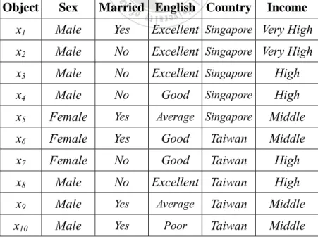
(31) similarity SimM ( Income, Children ) for the two attributes Income and Children is calculated as (0.875+0.625)/2, which is 0.75.. 3.3 Generalized Attribute Similarity Based on Majority Sets In general, attributes can be divided into three types: categorical, binary and ordinal. For example, the attributes Sex and Country in Table 3.2 are categorical; Married is binary; English and Income are ordinal. Table 3.2: A simple information system to evaluate the dependency. Object. Sex. Married English Country. x1. Male. Yes. Excellent Singapore Very High. x2. Male. No. Excellent Singapore Very High. x3. Male. No. Excellent Singapore. x4. Male. No. x5. Female. Yes. x6. Female. Yes. Good. Taiwan. Middle. x7. Female. No. Good. Taiwan. High. x8. Male. No. Excellent Taiwan. High. x9. Male. Yes. Average. Taiwan. Middle. x10. Male. Yes. Poor. Taiwan. Middle. Good. Singapore. Average Singapore. Income. High High Middle. For the binary or categorical attribute, two attribute values are regarded absolutely different if they are not the same. For an ordinal attribute, however, the difference between. 22.

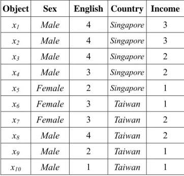
(32) two values should be evaluated according to their orders. Take the attribute English in Table 3.2 as an example. The difference between Excellent and Good is smaller than that between Excellent and Poor. In the last section, we propose a measure of attribute similarity based on the majority set. That method assumes the difference between any two attribute values is either 0 or 1 (i.e. the same or absolutely different) no matter what the attribute type is, in order to simplify the problem. Obviously, it is not desirable when some ordinal attributes appear, because the results from discretization may greatly affect the evaluated similarity. In this section, we thus propose another evaluation measure for attribute similarity, which is more general than the last method. The advantages of this method are: (1) the difference between two attribute values is not so rigid, and (2) the attribute similarity is less sensitive to the error from discretization. Before the dependency is calculated, the values of each ordinal attribute should be mapped to ranks (orders). For example, the information system in Table 3.2 is transformed into Table 3.3. Table 3.3: The transformed table of Table 3.2. Object. Sex. English Country Income. x1. Male. 4. Singapore. 3. x2. Male. 4. Singapore. 3. x3. Male. 4. Singapore. 2. x4. Male. 3. Singapore. 2. x5. Female. 2. Singapore. 1. x6. Female. 3. Taiwan. 1. x7. Female. 3. Taiwan. 2. x8. Male. 4. Taiwan. 2. x9. Male. 2. Taiwan. 1. x10. Male. 1. Taiwan. 1. 23.

(33) In Table 3.3, the set of values for attribute English includes Poor, Average, Good and Excellent. These values are thus mapped to {1, 2, 3, 4}. Similarly, the set of values for Income include Middle, High and Very High, which are then mapped to {1, 2, 3}. An evaluation of the dependency degree between two attributes is then defined as follows: DepM + ( Ai , A j ) =. ⎛ λ | X (vis ∧ v jt ) | ⎞ ⎜ | X ( v v ) | ∧ + ∑ ∑ Δ v , v ⎟⎟ , im jt N v jt ∈V j vim ∈Maj Ai ( v jt ) ⎜ vis ∈Vi \{vim } is im ⎝ ⎠ 1. ×. max. (. ). where DepM + ( Ai , A j ) is the dependency degree that attribute Ai depends on attribute Aj, N is the total number of objects, λ is the coefficient (fraction) for counting the objects which are. (. not major ones, 0≦λ＜1, and Δ vis , vim. ). represents the difference between two distinct. (. values of attribute Ai. Note that the computation of Δ vis , vim. ). depends on the type of. attribute Ai and is divided into the following cases: (1). (. ). Attribute Ai is binary or categorical. In this case, Δ vis , vim = 0 if the values vis. (. ). and vim are the same, and Δ vis , vim =1 otherwise. (2). (. Attribute Ai is ordinal. In this case, Δ vis , vim. ). equals the absolute value from the. difference of the ranks of vis and vim. For example, the difference Δ (English = 2, English = 4) can be computed as |2－4|=2.. The coefficient λ, on the other hand, is regarded as a weight of the objects except the major objects. The smaller λ is, the less important those objects are. Actually, this formula is the general form of the major dependency. That is, the inner summation is eliminated if λ is set as 0. Basically, the dependency DepM + ( Ai , A j ) involves four cases: ordinal to ordinal,. 24.

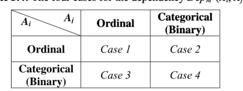
(34) ordinal to categorical (binary), categorical (binary) to categorical (binary), and categorical (binary) to ordinal. These four cases are shown in Table 3.4.. Table 3.4: The four cases for the dependency DepM+(Ai, Aj). Ordinal. Categorical (Binary). Ordinal. Case 1. Case 2. Categorical (Binary). Case 3. Case 4. Ai. Aj. For Cases 1 and 2, since attribute Ai is ordinal, the coefficient λ should be given in advance. For Cases 3 and 4, since attribute Ai is categorical or binary, the coefficient λ should be set as 0 to eliminate the inner summation. Below, some examples are given to illustrate the cases. Take the dependency DepM + ( Income, Country ) (i.e. Case 2) as an example. Since there are two possible values of Country, both the conditions Country = Singapore and Country = Taiwan. should. be. considered.. Assume. λ. is. set. at. 0.5.. The. dependency. DepM + ( Income, Country ) is calculated by the following steps.. (1) Since MajIncome(Country = Singapore) is {3, 2}, the set of objects in X(Country = Singapore) is analyzed to determine which value can get a higher dependency degree. For Income = 3: | X ( Income = 3 ∧ Country = Singapore) | +. +. 0.5× | X ( Income = 2 ∧ Country = Singapore) |. 0.5× | X ( Income = 1 ∧ Country = Singapore) | 1− 3. 25. 2−3 = 3.25.

(35) For Income = 2: | X ( Income = 2 ∧ Country = Singapore) | +. +. 0.5× | X ( Income = 3 ∧ Country = Singapore) |. 0.5× | X ( Income = 1 ∧ Country = Singapore) | 1− 2. 3−2 = 3.5,. The larger one (=3.5), which is “if Country = Singapore then Income = 2”, can get the higher dependency evaluation. (2) Similarly, consider another condition that Country = Taiwan as follows: | X ( Income = 1 ∧ Country = Taiwan) | +. 0.5× | X ( Income = 2 ∧ Country = Taiwan) | 2 −1. = 4.. (3) The dependency DepM + ( Income, Country ) is computed as: DepM + ( Income, Country ) =. 1 × (3.5 + 4) . 10. The computation of DepM + (Country, Income) (i.e. Case 3) is similar to that of DepM + ( Income, Country ) . There are three conditions which should be considered due to the. three values {1, 2, 3} of Income. In addition, since Country is a categorical attribute, the coefficient λ should be set at 0. The dependency DepM + (Country, Income) can be calculated in the same way. In summary, the computation of the dependency DepM + ( Ai , A j ). can be. divided into two situations. The first one is that the pre-attribute, Ai, is ordinal (i.e. Cases 1 and 2); the other one is that the pre-attribute is binary or categorical (i.e. Cases 3 and 4). We ignore the effect that the post-attribute (Aj) is ordinal. The dependency degree is not symmetric, such that the condition DepM(Aj, Ai) = DepM(Ai, Aj) is not always valid. The average value of DepM(Ai, Aj) and DepM(Aj, Ai) is thus used to represent the similarity of the two attributes Ai and Aj. Therefore, the proposed similarity 26.

(36) measure, denoted Sim(Ai, Aj), for a pair of attributes Ai and Aj is defined as follows: SimM ( Ai , Aj ) =. 1 ( DepM + ( Aj , Ai ) + DepM + ( Ai , Aj ) ) . 2. 27.

(37) CHAPTER 4 Attribute Clustering with Pre-Defined Cluster Numbers In this chapter an attribute clustering method based on k-medoids is proposed to partition the attributes into k clusters according to the dependency between each pair of attributes. It also uses a better search strategy to find centers (representative attributes) in a dense region, instead of random selection in k-medoids. After the attributes are partitioned into k clusters, each cluster can thus be represented by its representative attribute. The whole feature spaces can thus be greatly reduced.. 4.1 The Basic Concepts of the Proposed Algorithm For most clustering approaches, the distance between two objects is usually adopted as a measure for representing their dissimilarity, which is then used for deciding whether the objects belongs to the same cluster or not. In this thesis, the attributes, instead of the objects, are to be clustered. The conventional distance measures such as Euclidean distance or Manhattan distance are thus not suitable since the attributes may have different formats of data, which are hard to compare. For example, assume there are two attributes, one of which is age and the other is gender. It is thus hard to compare the two attributes via the traditional distance measure. Below, a measure based on the concept of relative data dependency is proposed to achieve it. It was proposed by Han et al. [17] and can be thought of as a kind of similarity degrees.. 28.

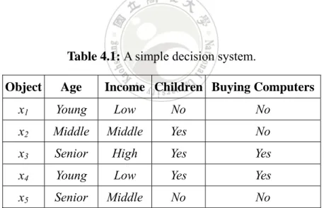
(38) Given two attributes Ai and Aj, the distance (dissimilarity) measure for the pair of attributes Ai and Aj is thus proposed as follows: d ( Ai , Aj ) =. 1 . Avg ( Dep( Ai , Aj ), Dep( A j , Ai )). where the distance d(Ai, Aj) is the inverse of the similarity Sim(Ai, Aj). Note that we can also use the other two evaluation methods for attribute similarity, and take the reciprocal as the distance, too. Take the distance between the two attributes Age and Income in Table 4.1 as an example. Since |ΠAge (U )| = 3, |ΠChildren (U )| = 2 and |ΠAge, Children (U )| = 5, the relative dependency degrees Dep(Age, Children) and Dep(Children, Age) are 0.6 and 0.4, respectively. The distance d(Age, Children) is thus 1/Avg(0.6, 0.4), which is 2.. Table 4.1: A simple decision system. Object. Age. Income Children Buying Computers. x1. Young. Low. No. No. x2. Middle. Middle. Yes. No. x3. Senior. High. Yes. Yes. x4. Young. Low. Yes. Yes. x5. Senior. Middle. No. No. 4.2 The Proposed Algorithm In this section, an attribute clustering algorithm called Most Neighbors First (MNF) is proposed to cluster the attributes into a fixed number of groups. Assume the number k of. 29.

(39) desired clusters is known. Some preprocessing steps such as removal of inconsistent or incomplete tuples and discretization of numerical data are first done. After that, the proposed MNF attribute clustering algorithm is used to partition the feature space into k clusters and output the k representative attributes of the clusters. The proposed clustering algorithm MNF is based on the k-medoids approach. Unlike the k-means approach, the proposed algorithm always updates the centers by some existing objects. Besides, it uses a better search strategy to find centers in a dense region, instead of random selection in k-medoids. The proposed algorithm MNF consists of two major phases: (1) reassigning the attributes to the clusters and (2) updating the centers of the clusters. In the first phase, the proposed distance measure is used to find the nearest center of each attribute. The attribute is then assigned to the cluster with that center. In the second phase, each cluster Ci uses a searching radius ri to find the neighbors of the attributes in Ci. The attribute with the most neighbors in a cluster is then chosen as the new center. The proposed algorithm is described in details below.. The MNF attribute clustering algorithm:. Input: An information system I = (U, A∪{d}) and the number k of desired clusters. Output: k appropriate attribute clusters with their representative attributes. Step 1 : Randomly select k attributes {A1c, A2c, … , Akc} as the initial representative attributes. (centers) in the k clusters, where Atc stands for the representative attribute (center) of the t-th cluster Ct, Atc ∈ A. Denote Ac = {A1c, A2c, … , Akc} ⊆ A as the initial representative attribute set.. 30.

(40) Step 2 : For each non-representative attribute Ai ∈ A－Ac, compute the expanded relative. dependency (distance) d(Ai, Atc) between attribute Ai and each representative attribute Atc as: d ( Ai , Atc ) =. 1 , Avg ( Dep ( Ai , Atc ), Dep ( Atc , Ai )). where Dep(Ai, Atc) represents the relative dependency degree of Ai with regard to Atc and Dep(Atc, Ai) represents the relative dependency degree of Atc with regard to Ai, t ∈ {1, 2, ... , k} . Step 3 : Allocate all non-center attributes to their nearest centers according to the distances. found in step 2. Collect a center attribute with its allocated attributes as a cluster. Step 4 : For each cluster Ct, calculate the distances between any two different attributes. within Ct. Step 5 : Calculate the radius rt of each cluster Ct as:. rt =. ∑d ( A. t ,i. i≠ j. C2nt. , At , j ) ,. where d(At,i, At,j) is the distance between any two attributes At,i and At,j within the cluster Ct, nt is the number of attributes within Ct, and C2nt is the number of attribute pairs in the cluster, which is. nt (nt − 1) . 2. Step 6 : For each attribute At,i (including the center Atc) within a cluster Ct, find the set of. 31.

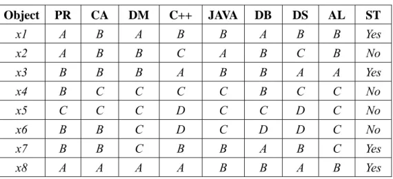
(41) attributes (called Near(At,i)) with their distances from At,i within rt. That is: Near ( At , i ) = { At , j At , j ∈ Ct and d ( At , i , At , j ) ≤ rt }.. Step 7 : For each cluster Ct, find the attribute At,l with the most attributes in its Near set. Set c At,l as the new center At of Ct.. Step 8 : Repeat Steps 2 to 7 until the clusters have converged. Step 9 : Output the final clusters and their centers as the representative attributes.. After Step 9, k clusters of attributes are formed and k representative attributes for the feature space are found.. 4.3 An Example In this section, a simple example is given to show how the proposed algorithm can be used to cluster the attributes. Table 4.2 shows the scores of eight students. There are eight condition attributes A = {PR, CA, DM, C++, JAVA, DB, DS, AL}, respectively standing for the eight subjects: Probability, Calculus, Discrete Mathematics, C++, JAVA, Database, Data Structure and Algorithms. The values of the condition attributes are {A, B, C, D}, which stand for the grade levels of a subject. There is one decision attribute {ST}, which stands for {Study for Master Degree} and has two possible classes {Yes, No}. In this example, the number of clusters is set at 2 (i.e. k = 2). For the set of data, the proposed algorithm proceeds as follows.. 32.

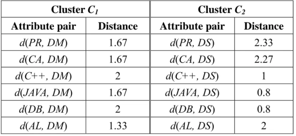
(42) Table 4.2: An example for attribute clustering. Object. PR. CA. DM. C++. JAVA. DB. DS. AL. ST. x1. A. B. A. B. B. A. B. B. Yes. x2. A. B. B. C. A. B. C. B. No. x3. B. B. B. A. B. B. A. A. Yes. x4. B. C. C. C. C. B. C. C. No. x5. C. C. C. D. C. C. D. C. No. x6. B. B. C. D. C. D. D. C. No. x7. B. B. C. B. B. A. B. C. Yes. x8. A. A. A. A. B. B. A. B. Yes. Step 1: k attributes are randomly selected as the initial centers of the clusters. In this. example, k is set at 2. Assume that the two attributes DM and DS are selected as the initial centers of the two clusters C1 and C2, respectively. Step 2: The distances (dissimilarities) between each non-center attribute and each center. are calculated. Take the distance between PR and DM as an example. Since |ΠPR| = 3, |ΠDM| = 3 and |ΠPR, DM| = 5, the relative dependency degrees Dep(PR, DM) is calculated as 0.6 and Dep(DM, PR) is 0.6 as well. The distance between the two attributes is thus calculated as: d ( PR, DM ) =. 1 = 1.67 . Avg (0.6, 0.6 ). All the distances between non-center attributes and representative centers are shown in Table 4.3.. 33.

(43) Table 4.3: The distances between non-center attributes and representative centers. Cluster C1. Cluster C2. Attribute pair. Distance. Attribute pair. Distance. d(PR, DM). 1.67. d(PR, DS). 2.33. d(CA, DM). 1.67. d(CA, DS). 2.27. d(C++, DM). 2. d(C++, DS). 1. d(JAVA, DM). 1.67. d(JAVA, DS). 0.8. d(DB, DM). 2. d(DB, DS). 0.8. d(AL, DM). 1.33. d(AL, DS). 2. Step 3: All non-center attributes are allocated to their nearest centers. Thus, cluster C1. contains {PR, CA, AL, DM} and cluster C2 contains {C++, JAVA, DB, DS}. Step 4: The distances between any two different attributes in the same clusters are. calculated. The results are shown in Table 4.4.. Table 4.4: The distances between any two attributes within the same clusters. Within cluster C1. Within cluster C2. Attribute pair. Distance. Attribute pair. Distance. d(PR, DM). 1.67. d(C++, DS). 1. d(PR, AL). 1.33. d(C++, DB). 1.25. d(CA, AL). 1.67. d(JAVA, DB). 2. d(PR, CA). 1.67. d(C++, JAVA). 1.67. d(CA, DM). 1.67. d(JAVA, DS). 1.25. d(AL, DM). 1.33. d(DB, DS). 1.25. 34.

(44) Step 5: The searching radius of each cluster is calculated. Take the cluster C1 as an. example. It includes 4 attributes {PR, CA, AL, DM}. The distances between each pair of attributes in C1 are {1.67, 1.67, 1.33, 1.67, 1.67, 1.33}. The radius r1 is then calculated as:. r1 =. 1.67 + 1.67 + 1.33 + 1.67 + 1.67 + 1.33 = 1.56 . 6. Step 6: The Near set of each attribute in a cluster is calculated. Take the attribute PR in. cluster C1 as an example. Its distance from the other three attributes CA, AL and DM in the same cluster are calculated as 1.67, 1.33 and 1.67. Near(PR) thus includes only the attribute AL since only AL is within the radius r1 (1.56), which is found from Step 5. Similarly, the Near sets of the other three attributes in the cluster C1 are found as follows: Near(CA) = φ , Near(AL) = {PR, DM}, and Near(DM) = {AL}.. Step 7: Since the attribute AL has the most attributes in its Near set for the cluster C1,. AL then replaces the attribute DM as the new center of C1. Similarly, the original center DS for C2 has the most attributes in its Near set. DS is thus still the center of C2. Step 8: Steps 2 to 7 are repeated until the two clusters no longer change. The final. clusters can thus be found as follows: C1 = {PR, CA, AL, DM}, with the center AL. C2 = {C++, JAVA, DB, DS}, with the center DS.. 35.

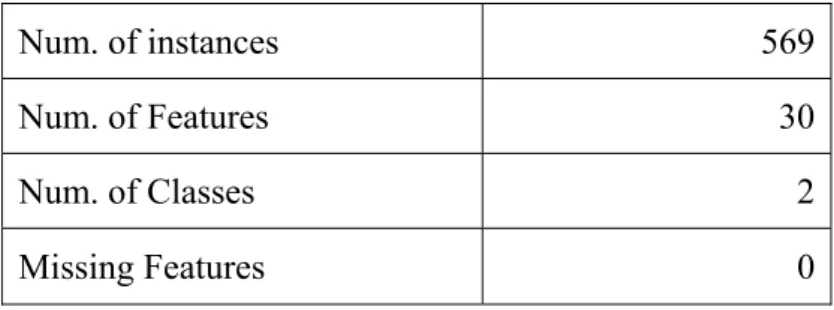
(45) Step 9: The final clusters and their centers as the representative attributes are then output.. The attributes in the same cluster can thus be considered to possess similar characteristics in classification and can be used as alternative attributes of the representative one. 1⎛ k 1 ⎜∑ k ⎜⎝ i =1 Ci. ⎞ d ( Aj , Ai ) ⎟ . ⎟ A j ∈Ci \ Ai ⎠. ∑. 4.3 Experimental Results In this section, the implement action of the proposed algorithms for clustering attributes with multiple cluster numbers is described. Note that the similarity measure, similarity based on majority sets, is used to compute the similarity between two attributes. The real world dataset, Wisconsin Breast Cancer Databases (wdbc), was used to verify our approach. The characteristics of the dataset are shown in Table 4.5. The experiments were implemented in C++ on an AMD Athlon 64 X2 Dual Core 3800+ personal computer with 2.01 GHz and 1 GB RAM.. Table 4.5: The characteristics of the dataset, wdbc.. Num. of instances. 569. Num. of Features. 30. Num. of Classes. 2. Missing Features. 0. 36.

(46) 0.7 0.6. Avg. S_in. 0.5 0.4. Equal Width Equal Freq. 0.3 0.2 0.1 0 1. 3. 5. 7. 9 11 13 15 17 19 21 23 25 27 Num. of cluster. Figure 4.1: The average S_in along with numbers of clusters.. In Figure 4.1, Sin denotes the average intra similarity for each cluster, it is defined as: 1⎛ k 1 . ⎜∑ k ⎜⎝ i =1 Ci. ⎞ Sim A A ( , ) ∑ j i ⎟. ⎟ A j ∈Ci \ Ai ⎠. 4.5 4. Avg. D_in. 3.5 3 2.5. Equal Width Equal Frequece. 2 1.5 1 0.5 0 1. 3 5. 7. 9 11 13 15 17 19 21 23 25 27 Num. of clusters. Figure 4.2: The average D_in along with numbers of clusters.. In Figure 4.2, D_in denotes the average intra distance (dissimilarity) for each cluster, it is. 37.

(47) defined as: 1⎛ k 1 ⎜∑ k ⎜⎝ i =1 Ci. ⎞ d ( Aj , Ai ) ⎟ ⎟ A j ∈Ci \ Ai ⎠. ∑. K=3. Times of being selected as centers. 90 80 70 60 50 40 30 20 10 0 1. 3. 5. 7. 9. 11. 13. 15. 17. 19. 21. 23. 25. 27. 29. 31. Attribute ID. Figure 4.3: The times of being selected as centers for each attribute for k=3.. K=6. Times of being selected as centers. 60 50 40 30 20 10 0 1. 3. 5. 7. 9. 11. 13. 15. 17. 19. 21. 23. 25. 27. 29. Attribute ID. Figure 4.4: The times of being selected as centers for each attribute for k=6.. 38.

(48) Times of beeing selected as centers. K=9 50 45 40 35 30 25 20 15 10 5 0 1. 3. 5. 7. 9. 11. 13. 15. 17. 19. 21. 23. 25. 27. 29. Attribute ID. Figure 4.5: The times of being selected as centers for each attribute for k=9.. According to the experimental results, the discretization is an important factor for our clustering algorithms. An unsuitable discretization method may destroy the dependency between a pair of attributes. Besides, the representative attribute could be arbitrary if the cluster number was larger. It is possible to define a criterion for selecting representative attributes, such as cost of the examination, ratio of missing values, and so on.. 39.

(49) CHAPTER 5 Attribute Clustering with Unknown Cluster Numbers In this chapter an attribute clustering method based on CAST is proposed. Although the number of clusters cannot be obtained, this algorithm can constructs clusters automatically. Given a threshold of affinity, the average similarity of the attribute pairs in the same cluster can be guaranteed to be within it.. 5.1 The Basics of the Proposed Algorithm In Chapter 4, we proposed an algorithm called the Most-Neighbor-First (MNF) to cluster attributes when the number of desired clusters has been known in advance. In many real applications, the appropriate number of attribute clusters may be hard to know in advance. Designing an attribute clustering algorithm when the number of clusters is not known in advance is thus important for feature selection and some other applications. We propose an approach for clustering attributes based on the CAST clustering algorithm, in which the average similarity of each cluster can be guaranteed to be within the given threshold γ. Besides, the majority similarity measure proposed in Section 3 is used to reflect the degree of similarity between two attributes.. 40.

(50) 5.2 The Proposed Algorithm In this section, we propose an approach for clustering attributes based on the CAST clustering algorithm, in which the average similarity of each cluster can be guaranteed to be above the given threshold γ. The notation used in the algorithm is first introduced below. Let A be the set of attributes to be clustered, C denote the set of clusters which have been constructed, Copen denote the cluster currently processed, Ac denote the set of representative attributes found, AU denote the set of attributes unassigned (not assigned) to any cluster, and k denote the current cluster number. Besides, the affinity of Ai, denoted a(Ai), represents the sum of the similarities between attribute Ai and the other attributes in the cluster Copen. That is: a(Ai) =. ∑ Sim. Ai ∈Copen A j ∈Copen − { Ai }. M. ( Ai , A j ) .. The proposed algorithm is described in details below.. The proposed attribute clustering algorithm with unknown cluster numbers:. Input: An information system I = (U, A∪{d}) and a similarity threshold parameter γ. Output: An appropriate number of attribute clusters, each with its representative attribute. Step 1 : Calculate the majority similarity SimM(Ai, Aj) of each pair of attributes Ai and Aj. Step 2 : Initially set C = φ , Ac = φ , copen = φ , AU = A, k = 1 and a(Ai) = 0 for 1≦i≦|A|.. 41.

(51) Step 3 : If Copen is empty, randomly choose and remove an attribute A+ from AU. ( AU = AU − { A+ } ) and add A+ to Copen (Copen = Copen∪{ A+ }); Otherwise, choose from AU the attribute A+ which will cause the maximum affinity in Copen; That is:. a( A+ ) = maxU a( Ai ) ; Ai ∈ A. If a( A+ ) ≥ γ Copen , then Copen = Copen∪{ A+ }, AU = AU − { A+ } , and do the next step; Otherwise, go to Step 6. Step 4 : Update the affinity of the old attributes in Copen due to the addition of A+ and. update the affinity of the remaining attributes in AU for later usage of finding another new A+ in Step 3. That is,. (. ). ∀Aj ∈ AU ∪ Copen − { A+ }, a( Aj ) = a( Aj ) + SimM ( Aj , A+ ) . Step 5 : Repeat Step 3 for adding more attributes to Copen until the maximum affinity of the. attributes in AU is less than γ Copen . Step 6 : Choose from Copen the attribute A− with the minimum affinity, that is:. a ( A− ) = min a ( Ai ) ; Ai ∈Copen. If a( A− ) < γ. (C. open. ). − 1 , then Copen = Copen－{ A− }, AU = AU ∪ { A− } , and do the. next step; Otherwise, go to Step 9. Step 7 : Update the affinity of the old attributes in Copen due to the removal of A− and. update the affinity of the old attributes in AU for later usage of finding another new. 42.

(52) A+ in Step 3. That is,. (. ). ∀Aj ∈ AU ∪ Copen − { A− }, a( Aj ) = a( Aj ) − SimM ( Aj , A− ) . Step 8 : Repeat Steps 3 to 7 until the attributes in Copen have converged. Step 9 : Construct the k-th cluster by setting Ck = Copen, C = C∪Ck. Step 10 : Choose the attribute A* with the largest affinity in Ck as the representative. attribute of Ck; That is, set Ac = Ac ∪ { A* } . Step 11 : Reset Copen as φ , a(Ai) = 0 for 1≦i≦|AU| and set k = k + 1. Step 12 : Repeat Steps 3 to 11 to generate the other clusters until the set AU is empty.. After Step 12, the clusters with their representative attributes can thus be found.. 5.3 An example In this section, a simple example is given to show how the proposed algorithm can be used to cluster the attributes. Table 5.1 is a decision system in which there are five condition attributes A = {SE, IN, TR, CH, AG} standing for Sex, Income, Transport, Children and Age respectively. The values of these attributes are {Male, Female}, {High, Middle, Low}, {Car, Bus, Train}, {Yes, No} and {Young, Middle, Senior}. Besides, there is a decision attribute PE standing for Keeping the Pet, and its possible values are {Yes, No}. Assume the similarity threshold parameter γ is set at 0.65. For the set of data, the proposed algorithm proceeds as follows.. 43.

(53) Table 5.1: An example for attribute clustering. Object. SE. IN. TR. CH. AG. PE. x1. Male. High. Car. Yes. Young. Yes. x2. Male. High. Bus. Yes. Senior. No. x3. Male. High. Bus. No. Middle. Yes. x4. Female. High. Train. No. Middle. No. x5. Female. Middle. Bus. No. Middle. No. x6. Female. Middle. Train. No. Senior. No. x7. Female. Middle. Car. Yes. Young. Yes. x8. Female. Low. Car. No. Young. Yes. Step 1: The majority similarity measure of each pair of attributes is calculated. Take the. similarity between CH and AG as an example. Since X ( AG = Young ∧ CH = Yes ) = 2 and X ( AG = Old ∧ CH = Yes ) = 1 , the majority set for CH = Yes on Age is Age = Young. That is,. Maj AG (CH = Yes ) = {Young}. Similarly, Maj AG (CH = No) = {Middle} can be found. The dependency degree Dep M ( AG , CH ) for the attribute CH to depend on AG is calculated as:. | X ( AG = Young ∧ CH = Yes ) | + | X ( AG = Male ∧ CH = No) | 8 2+3 = = 0.625. 8. Dep M ( AG, CH ) =. Similarly, the dependency degree DepM(CH, AG) for CH to depend on AG is calculated as 0.75. The majority similarity (SimM(CH, AG)) of the two attributes CH and AG is thus calculated as (0.625+0.75)/2, which is 0.688. The majority similarity values for the other pairs can be found in the same way. The resulting majority similarity values for all the pairs of attributes are shown in Table 5.2.. 44.