1
Deterministic Test Pattern Generation using
Segmented LFSR
Lung-Jen Lee1, Wang-Dauh Tseng, Rung-Bin Lin, and You-An Chen
Department of Computer Science & Engineering Yuan Ze University, Chung-li, Taiwan, 32026, ROC
1s959101@mail.yzu.edu.tw
Abstract — A new test data generation technique combining traditional internal liner feedback shift register (LFSR) with a specific polynomial LFSR, is presented in this work. The specific polynomial LFSR (SP-LFSR) method explores the distributions of 0’s and 1’s in each column and logically gathers the columns with mostly 0’s or 1’s for generation. This approach reduces more test time than the traditional LFSR does. Most previous techniques reduce test application time at the expense of hardware overhead. In our new method, we analyze the test data and reorder the scan chain into two parts while feeding the test data. The hardware overhead is low, only some inverters and XOR gates are required.
Index terms — specific polynomial LFSR, test data
generation
1.INTRODUCTION
Built-in self-test (BIST) is a technique that makes circuits test itself without using automatic test equipment (ATE). Linear feedback shift register (LFSR) are usually used as test pattern generator (TPGs) in low overhead BIST schemes. This is due to the fact that an LFSR can be built with little area overhead. By now, many BIST methods were developed [1]-[5], all of them trying to find some trade-off between these four mutually antipodal aspects: the fault coverage, test time, the area overhead and the BIST design time. Attainment of high fault coverage with sequences is the main objective of BIST techniques.
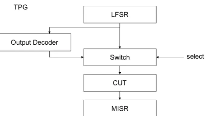
Achieving high fault coverage for CUTs that contain many random pattern resistant faults (RPRFs) only with pseudorandom patterns generated by an LFSR often requires unacceptably long test sequences and results in prohibitively long test time. A combination of a pseudo-random and deterministic BIST is being referred to as a mixed-
LFSR Switch CUT MISR Output Decoder TPG select
Figure 1. Mixed-Mode Architecture
mode BIST, the architecture shows in Figure 1. To support the mixed-mode testing, the test is divided into two disjoint phases, i.e., the pseudo-random phase and the deterministic phase. If test application time is long during pseudo-random phase, the output decoder is smaller. If test application time is short during pseudo-random phase, the output decoder is larger. Several techniques have been proposed to address this problem, e.g., reseedable and/or reconfigurable LFSRs in [6]-[8], bit-fixing and bit-flopping techniques in [2] and [4], and column-matching technique in [9] and [10].
Scan-Based BIST can be simply classified into two types of test schemes: test-per-scan scheme and test-per-clock scheme. In test-per-clock BIST, a test pattern is applied and the test response is captured every clock cycle. Using test-per-clock scheme to generate test patterns needs fewer test patterns to reach the same fault coverage than the test-per-scan test scheme does. The architecture shows in Figure 2.
2 LFSR CUT … … MISR
Figure 2. Test-per-clock BIST architecture LFSRs can be simply classified into two types: internal LFSR and external LFSR. In internal LFSR, inputs of selected stages Di, given by the feedback
polynomial of the LFSR, are driven by two-input XOR gates whose inputs are driven by outputs of preceding LFSR stages Di-1 and the last stage Dn.
Hence, unlike the external LFSR, Qi(t) can be
different from Qi-1(t-1) in an internal LFSR if the
input of Di is connected to the output of Di-1
through a two-input XOR gate whose other input is driven by the output of the last stage(Dn) of the
LFSR. The architectureof internal LFSR is shown
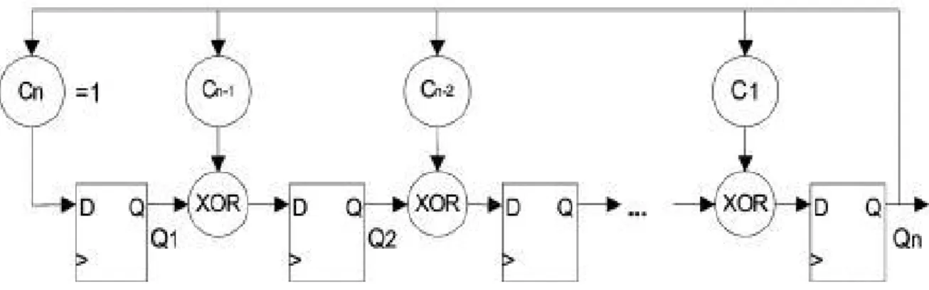
Figure 3. Ring counter architecture and test sequence
in Figure 3. The ring counter is a special case of internal LFSR, the polynomial is XN+1, as shown in Figure 4.
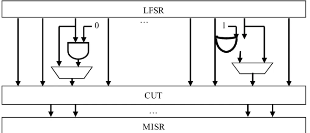
Figure 5 shows an architecture of mixed-mode BIST. First, LFSR is used to generate the test pattern to detect the easy-detect fault, and then bit-fixing technique is performed to fix random value to 0 or 1.
3 LFSR … 0 CUT MISR … 1
Figure 5. Mixed-mode architecture Table 1. Test cube sets and detection probability
C c6 c5 c4 c3 c2 c1 dp
P1 1 X 0 1 X 0 1/24
P2 X 1 0 0 0 X 1/24
P3 1 X X 0 X 1 1/23
P4 0 1 X 0 0 1 1/25
Table 2. The new detection probability after bit-fixing is used C c6 c5 c4 c3 c2 c1 dp P1 1 1 0 1 0 0 1/23 P2 X 1 0 0 0 X 1/2 P3 1 1 0 0 0 1 1/23 P4 0 1 0 0 0 1 1/23
Table 1 shows the test cube sets, input c2 is always assigned 0 or don’t care bit (X) in Table 1. Therefore, input c2 is assigned to 0 in every test cycle. Similarly, input c4 is assigned to 0 and c5 is assigned to 1. In order to lock the value, the authors use an AND gate to lock value to 0 and use an OR gate to lock value to 1.
The dp is detection probability, and it is simply given by 1/2the number of care bits. If input can be fixed to 0(1) (with underline in Table 2) without making any fault untestable, the dp can be increased as shown in Table 2.
2. PROPOSED METHOD
We proposed a methodology to reduce test application time during the test mode. Several techniques have been proposed to address this problem. The mixed-mode BIST is used to detect
hard-to-detect fault which is undetectable after RTPG patterns are applied. If test application time is long during pseudo-random phase, the output decoder is smaller. If test application time is short during pseudo-random phase, the output decoder is larger. The proposed method is to reduce application time that test patterns generated by the pseudo-random phase detect easy-to-detect faults. The proposed test scheme uses traditional LFSR and SP-LFSR to generate test patterns to detect easy-to-detect faults, the architecture as shown in Figure 6. The characteristic of internal LFSR is that scan cells would be partitioned according to the distribution of number 0 and 1. The ratio of don’t care-bit in the test patterns is very important when the scan chain is partitioned. If the don’t care-bit ratio is low, it is hard to find columns that generated by SP-LFSR.
Let us consider an RTPG that uses an internal LFSR where initial value D1D2…DN is 100…0.
The Dn is 0 from the first cycle to the (n-1)th cycle,
so the input of stage Di, where i =2,3,…,n, is
directly driven by the output of the preceding LFSR stage Di-1 and the D1 is driven by the Dn during the
(n-1) cycle. As show in Figure 7(a), it is the sequence that test patterns generated by the RTPG when LFSR size is 4 and seed is 1000. Internal LFSR has a special characteristic that there is only single 1 from P1 to P4 in the test patterns. Another characteristic of LFSR is to generate the shortest test pattern sequence when polynomial is Xn+1 and the seed is 100…0, we call the architecture as ring counter. Fig 7.(b) show the result when polynomial is X4+1 and seed is 1000. The rule is true when n > 1.
4
LFSR I LFSR II
CUT
MISR …
Figure 6. Proposed Architecture
(a) (b)
Figure 7(a). LFSR size is 4 and seed is 1000. (b) Polynomial is X4+X3+ X2+X+1 and seed 1000
Table 3. Test cubes
C1 C2 C3 C4 C5 C6 C7 C8 C9 C10 P1 1 0 X 1 1 X X X 1 X P2 0 0 X 1 0 0 0 1 X X P3 X 0 X 1 1 X X X 0 X P4 X 0 0 0 1 X 0 1 0 X P5 X 0 X X X 1 1 1 X 1 P6 1 X 0 1 X 1 1 X X X P7 X 0 X X X 0 1 X X 0 P8 1 0 X 0 X X X X X X P9 X 0 X X 1 X X 0 X 1 P10 X 1 0 1 1 X 1 0 X X
There are a lot of don’t-care bits in test patterns, if we don’t merge the test patterns. We try to collect columns that can be generated by SP-LFSR, and then use traditional LFSR and SP-LFSR to generate each test pattern. For example as show in Table 3, there are 10 test cubes and each test cube has 10 bits.
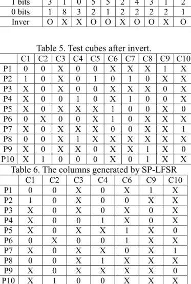
Firstly, we count the number of 0 and 1 in each column (Table 4). If the number of 1’s is more than
Table 4. The number of 1 and 0 in each column.
C1 C2 C3 C4 C5 C6 C7 C8 C9 C10
1 bits 3 1 0 5 5 2 4 3 1 2
0 bits 1 8 3 2 1 2 2 2 2 1
Inver O X X O O X O O X O
Table 5. Test cubes after invert.
C1 C2 C3 C4 C5 C6 C7 C8 C9 C10 P1 0 0 X 0 0 X X X 1 X P2 1 0 X 0 1 0 1 0 X X P3 X 0 X 0 0 X X X 0 X P4 X 0 0 1 0 X 1 0 0 X P5 X 0 X X X 1 0 0 X 0 P6 0 X 0 0 X 1 0 X X X P7 X 0 X X X 0 0 X X 1 P8 0 0 X 1 X X X X X X P9 X 0 X X 0 X X 1 X 0 P10 X 1 0 0 0 X 0 1 X X
Table 6. The columns generated by SP-LFSR
C1 C2 C3 C4 C6 C9 C10 P1 0 0 X 0 X 1 X P2 1 0 X 0 0 X X P3 X 0 X 0 X 0 X P4 X 0 0 1 X 0 X P5 X 0 X X 1 X 0 P6 0 X 0 0 1 X X P7 X 0 X X 0 X 1 P8 0 0 X 1 X X X P9 X 0 X X X X 0 P10 X 1 0 0 X X X
0’s, the column would be inverted to increase the number of columns that can be generated by SP-LFSR. Table 5 shows the test patterns after invert.
Secondly, we collect columns that can be generated by SP-LFSR. We reorder the columns according to the number of 1’s in each column. In this case, the sequence is C3, C1, C2, C5, C9, C10, C4, C6, C7, C8. We select C3 at first and find no any row conflict with C, so, we add the C3 to S. Because the C3 has no 1 in any row, we update C = {0,0,0,0,0,0,0,0,0,0}. After that we select C1, and find no any row conflict with C. So, we add C1 to S, and update C={0,1,0,0,0,0,0,0,0,0}. And then, we add S2 to S, and update C={0,1,0,0,0,0,0,0,0,1}. P1: 1 0 0 0 P2: 0 1 0 0 P3: 0 0 1 0 P4: 0 0 0 1 P5: … Test patterns P1: 1 0 0 0 P2: 0 1 0 0 P3: 0 0 1 0 P4: 0 0 0 1 P5: 1 0 0 0 Test patterns
5 When C5 is selected, we find the second row is 1 which is conflict with C, so, we don’t add C5 to S. Finally, we find the set S = {C1, C2, C3, C4, C6, C9, C10}. As show in Table 6, C={1,1,0,1,1,1,1,1,0,1}.
The final result is shown in Fig 8. The tradition method uses 121 cycles to detect all cubes, but our method only uses 44 cycles.
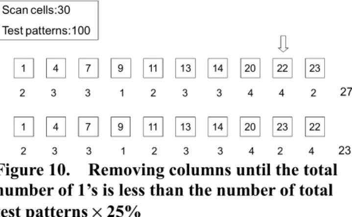
The test application time is affected by the number of 1 in C. The reason for the longer test application time is illustrated by Table 7. In Case I, the test cube is detected when the test pattern is 0010000000. In Case II, the test cube is detected when test patterns are 0100000000, 0001000000, 0000100000, 0000000100 and 0000000001. The authors remove columns which the number of 1 is more than the number of total test patterns × 5%, as shown in Figure 9. Another, the authors remove columns until the total number of 1 less than the number of total test patterns × 25%, as shown in Figure 10.
A special polynomial LFSR used to advance the detection probability, the polynomial is XN+XN/2+1,
SP-LFSR LFSR
I1 I2 I3 I4 I5 I6 I7 I8 I9 I10 CUT
Figure 8. The final link
Table 7. The test cubes and the corresponding detection probability by Ring Counter.
Test cubes probability detection Case I 0 X 1 X X 0 0 X 0 X 1/10 Case II 0 X 0 X X 0 0 X 0 X 5 /10 1 2 4 5 6 9 3 7 8 10 2 3 3 1 2 7 3 5 8 4 1 2 4 5 6 3 7 8 9 10 2 3 3 1 2 3 5 8 7 4 Scan cells:10 Test patterns:100
Figure 9. Removing the columns which the number of 1’s is more than the number of total test patterns × 5% 1 4 7 9 11 13 14 20 22 23 2 3 3 1 2 3 3 4 4 2 Scan cells:30 Test patterns:100 2 3 3 1 2 3 3 4 2 4 1 4 7 9 11 13 14 20 23 22 27 23 Figure 10. Removing columns until the total number of 1’s is less than the number of total test patterns × 25%
as shown in Figure 11. Figure 10 shows the test sequence increases from N to 3/2N. The hardware overhead is an XOR gate. The Max transition increases from 2 to 4. The detection probability increases as shown in Figure 12.
Ring Counter SP-LFSR Cycle N 3/2N Hardware 0 1 Max Transition 2 4 + Pattern: 1 0 0 0 0 0 0 1 0 0 0 0 0 0 0 0 0 1 1 0 0 1 0 0 0 1 0 0 1 0 0 0 1 0 0 1 … Polynomial = Xn+Xn/2+1
6
Test cube detection probability
Case I 0 X 1 X X 0 0 X 0 X 2/15 Case II 0 X 0 X X 0 0 X 0 X 6/15 0000000001 0000000010 0000000100 0000001000 0000010000 0000100000 0001000000 0010000000 0100000000 1000000000 Case I: 0000000001 0000000010 0000000100 0000001000 0000010000 0000100000 0001000000 0010000000 0100000000 1000000000 Case II: 0000100001 0001000010 0010000100 0100001000 1000010000 0000100001 0001000010 0010000100 0100001000 1000010000
Figure 12. The detection probability using SP-LFSR
3.EXPERIMENTAL RESULTS
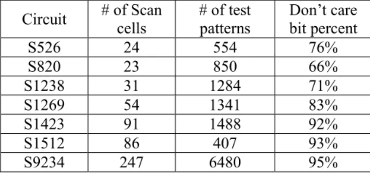
The experiments presented in the paper are focused on reducing the test application time and low hardware overhead. This work is implemented by C++ language and is performed on ISCAS’89 benchmarks. Table 8 shows the characteristics of the benchmark. The table shows the number of scan cells, test patterns in each circuit. It also shows the percentage of don’t care bits in each circuit.
The experiments were designed to detect the easy-to-detect faults. In order to compare the test application time applied by ring counter, SP-LFSR and Tradition LFSR test sequence, the same fault coverage is set for each circuit.
Table 9 compares the application time applied by test patterns generated by ring counter with those generated by Traditional LFSR. The column labeled Total patterns shows the number of total test patterns for each benchmark circuit and column labeled Hit patterns shows the number of test patterns detected to each benchmark circuit. The labeled FC shows fault coverage achieved by test sequence. In order to compare application time applied candidly, the authors set the same seed (10…00) and polynomial of Traditional LFSR (Xn+X+1). The column labeled Traditional LFSR
shows the length of the test sequence that Tradition LFSR applied to each circuit and column ring counter shows the length of the test sequence that ring counter applied to each circuit. The column labeled Test time reduction shows the improvement in test application time using ring counter. The column labeled XOR gates shows the number of total XOR gates used to each benchmark circuit. Table 10 compares the application time applied by test patterns generated by SP-LFSR with those generated by Traditional LFSR. Table 11 compares the fault coverage achieved by test pattern generated by ring counter with those generated by Traditional. The column labeled Time shows the test application time applied to each circuit. The column labeled Traditional LFSR FC(%) shows fault coverage achieved using
Table 8. The characteristics of the benchmarks
Circuit # of Scan cells # of test patterns Don’t care bit percent S526 24 554 76% S820 23 850 66% S1238 31 1284 71% S1269 54 1341 83% S1423 91 1488 92% S1512 86 407 93% S9234 247 6480 95%
7
Table 9. Test length comparison between Ring Counter with Traditional LFSR
Circuit #Total patterns #Hit patterns #FC Traditional LFSR Ring Counter Improve (%) #XOR gates S526 554 553 99.8% 23559 19548 17.03 1 S820 850 850 100% 92326 27292 70.44 1 S1238 1284 1164 90.6% 27067 7152 73.58 1 S1269 1341 1274 95.0 542119 18556 96.58 1 S1423 1488 1453 97.6% 476030 107230 77.47 1 S1512 407 375 92.1% 16386 2293 86.01 1 S9234 6480 5798 89.4% 3497280 360317 89.70 1 Average 72.97
Table 10. Test length comparison between SP-LFSR with Traditional LFSR
Circuit #Total patterns #Hit patterns #FC (%) Tradition Method SP-LFSR Improve (%) #XOR gates S526 554 553 99.8 23559 16273 30.93 2 S820 850 850 100 92326 15340 83.38 2 S1238 1284 1164 90.6 27067 7710 71.51 2 S1269 1341 1274 95.0 542119 18098 96.66 2 S1423 1488 1453 97.6 476030 103147 78.33 2 S1512 407 375 92.1 16386 2056 87.45 2 S9234 6480 5798 89.4 3497280 481511 86.23 2 Average 76.36
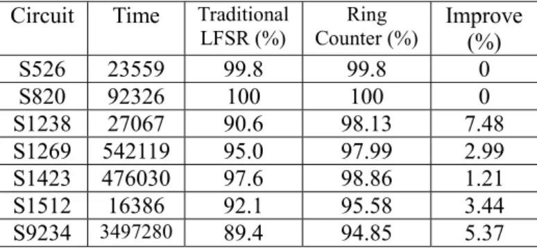
Traditional LFSR generator the test pattern by test sequence. The column labeled Ring Counter FC(%) shows fault coverage achieved using ring counter generator the test pattern by test sequence. The column labeled Improve shows the improvement in fault coverage using ring counter. Table 12 compares the fault coverage achieved by test pattern generated by SP-LFSR with those generated by Traditional.
4.CONCLUSIONS
In this paper, we propose a new architecture of test generation to reduce the test application time without sacrificing fault coverage. The scan chain is partitioned into two parts according to the distribution in number of 1’s and 0’s. Test data in the two parts are generated by the SP-LFSR and the traditional LFSR respectively. Results show the test application time can be reduced efficiently compared with traditional LFSR architecture.
Table 11. Fault coverage comparison between Ring Counter with Traditional LFSR
Circuit Time Traditional
LFSR (%) Ring Counter (%) Improve (%) S526 23559 99.8 99.8 0 S820 92326 100 100 0 S1238 27067 90.6 98.13 7.48 S1269 542119 95.0 97.99 2.99 S1423 476030 97.6 98.86 1.21 S1512 16386 92.1 95.58 3.44 S9234 3497280 89.4 94.85 5.37
Table 12. Fault coverage comparison between SP-LFSR with Traditional LFSR
Circuit Time Traditional
LFSR (%) SP-LFSR (%) Improve (%) S526 23559 99.8 99.8 0 S820 92326 100 100 0 S1238 27067 90.6 99.07 8.42 S1269 542119 95.0 98.14 3.14 S1423 476030 97.6 98.72 1.07 S1512 16386 92.1 95.82 3.68 S9234 3497280 89.4 94.24 4.76
8
REFERENCES
[1] V.K. Agrawal, C.R. Kime and K.K. Saluja. A tutorial on BIST, part 1: Principles, IEEE Design & Test of Computers, vol.10, No.1 March 1993, pp. 73-83, part 2:Applications, No.2 June 1993, pp. 69-77.
[2] H.J. Wunderlich and G. Keifer. Bit-Flipping BIST, Proc. ACM/IEEE International Conference on CAD-96 (ICCAD96), San Jose, California, November 1996, pp. 337-343. [3] N.A. Touba and E.J. McCluskey. Altering a
Pseudo-Random Bit Sequence for Scan-Based BISR, Proc. of ITC’96, PP. 167-175.
[4] N.A. Touba and E.J. McCluskey. Bit-Fixing in Pseudorandom Sequences for Scan BIST, IEEE TCAD, Vol. 20, No. 4, April 2001. pp 545-555. [5] M. Chatterjee and D.K. Pradhan. A BIST
Pattern Generator Design for Near-Perfect Fault Coverage, IEEE Transactions on Computers, vol. 52, no. 12, December 2003, pp. 1543-1558.
[6] S. Hellebrand, J. Rajski, S. Tarnick, S. Venkataraman, and B.Courtois, “Built-In test for circuits with scan base on reseeding of multiple-polynomial linear feedback shift registers,” IEEE Trans. Comput., vol. 44, no.2,
pp. 223-233, Feb. 1995.
[7] N. Zacharia, J. Rajski, and J. Tyszer, “Decompression of test data using variable-length seed LFSRs,” in Proc. IEEE 13th VLSI Test Symp., 1995, pp. 426-433.
[8] S. Hellebrand, J. Rajski, S. Tarnick, “Generation of vector patterns through reseeding of multiple-polynomial linear feedback shift registers,” in Proc. IEEE Int. Test Conf., 1992, pp. 120-129.
[9] Fišer, P., Hlavička, J., Kubátová, H.: “Column-Matching BIST Exploiting Test Don't-Cares“, Proc. 8th IEEE Europian Test Workshop, Maastricht, 2003, pp. 215-216
[10] Fišer, P., Kubátová, H.: “An Efficient Mixed-Mode BIST Technique“, Proc. 7th IEEE Design and Diagnostics of Electronic Circuits and Systems Workshop 2004, Tatranská Lomnica, SK, 18.-21.4.2004, pp. 227-230
[11] Seongmoon Wang, Sandeep K. Gupta, “LT-RTPG: A New Test-Per-Scan BIST TPG for Low Switching Activity,” IEEE Transactions on Computer-Aided Design of Integrated Circuits and Systems, vol. 25, no. 8, August 2006