APPROXIMATE SOLUTIONS FOR TRANSIENT-RESPONSE OF A SHELL AND TUBE HEAT-EXCHANGER

(1)

Approximate Solutions for Transient Response of a Shell and Tube Heat

Exchanger

K. S . Tan

Institute of Applied Chemistry, National Chiao Tung University, Hsinchu, Taiwan, R.O.C.

I. H.

Spinners

Department of Chemical Engineering and Applied Chemistry, University of Toronto, Toronto, Canada M5S 1Al

Approximate solutions for the transient response of a shell and tube heat exchanger to step change

in shell fluid temperature and tube fluid velocity are derived.

It has

been shown that other previously

published limited or approximate solutions are derivable from the exact solutions. T h e limiting

asymptotic “no wall” solutions for both response to shell fluid temperature and tube fluid velocity

change are also deducible from a limiting tube wall time constant solution. Some of the approximate

solutions presented include the use of simple exponential forms of equations that enable the quick estimation of the time required t o reach a given degree of approach to the final steady state. The error between the exact and the approximate exponential form of solutions are in most cases less than 2%. All the previous derived exact and approximate solutions presented here are applicable

to crosscurrent, cocurrent, or countercurrent flow heat exchangers with one infinite thermal capa-

citance rate fluid.

Introduction

The design, operation, and control of heat exchangers would be facilitated by equations describing the transient response. Unfortunately the basic dynamic equations in- volve simultaneous partial differential equations for which

the analytic solutions are complex and difficult to obtain.

In most cases, numerical methods such as method of characteristics (Tan and Spinner, 1984) are used to cal- culate the transient response for heat exchanger with cocurrent, crosscurrent, or countercurrent flow.

For the case of heat exchangers with one infinite capa-

citance rate fluid, London et al. (1959) present some results

from analog simulation. Myers et al. (1970) gave extensive

results from finite difference calculations. Rizika (1956) gave an exact analytic solution for this case, but the solution is applicable only for time less than one residence time. Limiting and approximate solutions were also

presented by London et al. (1959) and Myers et al. (1970).

All the above studies deal only with response to fluid temperature change.

Exact analytic solutions for the transient response of a shell and tube heat exchanger to change in both fluid temperature and tube fluid velocity changes have been previously published (Tan and Spinner, 1978). Shah

(1981) has statsd that these solutions are equally applicable

to a heat exchanger having an infinite capacitance rate

fluid. Graphs prepared from these exact solutions have

also been published (Tan and Spinner, 1978; Shah, 1981). The purpose of this paper is to present some useful approximate solutions which give results that are in good agreement with the exact solutions. The applicability of these solutions with regard to the values of the design

parameters will be investigated, and the magnitude of error

introduced compared to the exact solution will be dis-

cussed. Limiting asymptotic solutions as applied to the

case in which the product of Cf (limiting dimensionless tube wall time constant) becomes very small will be ex-

amined. It will be shown that all the previous published

approximate solutions for response to shell fluid temper-

ature change are directly derivable from these exact so-

lutions. It will be shown that the limiting “no wall” solution is obtainable from the approximate solution for a small value of the product Cf.

0888-5885/91/2630-1639$02.50/0

The use of a simple exponential form of equation as an approximate solution not only facilitates the evaluation

of the transient history of the exchanger but also provides

a simple method of estimating the time required to reach

a given degree of attainment of the final steady state. For compactness, all the derived new approximate solutions will be expressed in terms of the previous notation (Tan and Spinner, 1978).

Transient Response to Step Change in Shell Fluid Temperature

In a previous paper

Tan

and Spinner (1978) derived the

following exact solution to the transient response of step

change in shell fluid temperature:

exp

[

-a -

(if

-

- R1

)

(e*

-

+

where

U

is the fractional attainment of the final steady

state, with

R 1 = J[ 2 (1

+

Q)

+

[

(1

+

Q ) 2 - 4(1 T]l”] - f )

Since

C

is the dimensionless thermal capacity ratio of

tube wall to tube fluid and f is the fractional heat-transfer

(2)

1640 Ind. Eng. Chem. Res., Vol. 30, No. 7, 1991

resistance on the shell side, then Cf is the dimensionless

tube wall time constant and l/R1 and 1/R2 are the

"effective time constants" for the coupled tube fluid and wall system.

The normalized final steady state value is given by

P = 1

-

exp[-(l - fla]

The two mathematical functions

d1

and $ are defined

by

d l ( x , ~ ) = J'do(X,y) dX = 1 -

AXY)

dO(x,y) = exp(-x - ~ ) 1 ~ [ 2 ( x y ) ~ / ~ ] where

Both J and

#

can be easily generated by the following

simple algorithms:

X O = 1

-

exp(-x) and X k = kXk-l

-

x k exp(-x)

for k 1 1

X o = 1

-

exp(-x) and X k = xc - kXcl for k 2 1

Note that J is a well-known tabulated function whose

values are readily obtainable (Helfferich, 1962; Sherwood

et al., 1975). It was mentioned in the previous publication

(Tan and Spinner, 1978) that neglecting the term con-

taining the $ function would lead to at most 2% relative

error for a practical range of parameters. More specifically, the range was 1

<

a

<

3, C

<

3, f

<

0.2. Thus eq 1 without

the

#

term is a good approximation for design purposes

since J or

d1

are known tabulated functions and the nu-

merical evaluation could be readily carried out if tables

were available. Alternatively the J function could be easily

calculated with a programmable calculator or microcom- puter using the algorithms given.

For engineering application, it would be worthwhile to consider the possibility of using an equation that is in a simpler form. Myers et al. (1970) had successfully used a first-order exponential function to approximate the

transient response for 8* 1 1. They compared 27 cases of

solution with those obtained from a finite difference numerical method. The difference between the exponential form of equation and the finite difference solution was almost indistinguishable on the graphs presented. Since exact analytic solutions are available, it would not be difficult to compare the approximate solution for an extensive range of values of the parameters C, f , and a. The

method used by Myers et al. (1970) in formulating an

exponential form of equation as an approximating solution was followed. However, a more compact equation for the

evaluation of the constant used in the exponential function

was obtained. The derivation by Myers et al. was based on the exact solution for transient response for the first

time domain as presented by Rizika (1956). In this regard

it should be noted that the first three terms of eq 1 which

provide the first time domain

(e*

<

1) response are readily

rearranged in the following form:

1

U

= - 4 1

-

exp(-X)[sinh (X/Y)

+

cosh

(X/Y)])

(2)

II"

y=- R1

+

R2 = - 1

+

Cf

[

(

1 + -

kf

)2 -- 4(l& t 7 ] - 1 ' 2

%-R2 Cf

The f i s t three terms of eq 1 are thus identical with the analytical solution derived by Rizika (1956). However, eq

2 not only provides the exact solution for the first time

domain (8*

<

1) but also constitutes part of the solution

for the entire time domain. The approximate solution proposed by Myers et al. could thus be expressed in the following form using the present authors' notation:

(3)

U = 1 - (1 - U,) exp[-K(B* - l)]

An equivalent form of eq 3 is

U = U1

+

(1 - Ul)(l - exp[-K(B* - l)]) (3A)

with

where Ul is the fractional attainment of the final steady

state at one throughput time.

Since 1 - U , represents the fraction of remaining tran-

sient after one throughput time has elapsed, the second

term of eq 3A can be viewed as a simple exponential

growth function that describes the transients of the term

1 - U , for the time region of 8* 1 1. Equation 3 contains

only one adjustable parameter, K, and therefore can be

readily determined from one independent relationship. Myers et al. obtained the value of K by matching the

derivative of U with respect to 8* at 8* = 1. Since eq 3

is to be applied for the time domain of 8* 1 1, it would

be more appropriate to use the derivative evaluated from

eq 1 for matching purposes. After differentiating eq 1 for

8* 1 1 and letting 8* approach 1, the following value of K was obtained:

K = R1R2[ exp(-R2a)

-

exp(-Rla)] (4)

a

p(1 - Ui)(Rl

-

R2)

By substituting the values for

Ul

and

P

K =

R1R2[exp(-R2a) - exp(-Rla)]a

R1 exp(-R2a) - R2 exp(-Rla)

-

(Rl

-

R2) exp[-(1

-

t7.1

(4A) Myers et al. (1970) used Rizika's exact solution for the

first time domain for determining the slope at 8* = 1. The value of K expressed in the same hyperbolic functions but using the present authors' notation is

2C(1

-

f).

T"(1

-

UJ(1

+

cfl

K = - Y exp(-z) sinh

(Z/Y)

(4B)

where

1

+

Cf

z = -

2Cf a

and Y is defined in eq 2.

Equations 4 and 4B are identical; however, it is felt that

the form of eq 4 is more convenient to use. It is noted that

in eq 4 the "effective time constant" of the approximate

equation consists of P(1

-

Ul),

which is the fraction of

remaining transient after 8* 2 1 and the quantity, ( R ,

-

R2)/R1R2, which is the difference of the two "effective time

constants", l / R 1 and 1/RP The constant

K

incorporates

all the parameters C, f, and a. The fact that the derivatives dU/d8*lrll are identical when derived from both time

(3)

Limiting "No Wall" and Small Cf Solutions. For

extremely small values of

C

and f where both

C

and f are

finite, practically no transient exists after the first time domain. In such a case the

third

term in eq 6 could become

negligible and a two-term equation would be sufficient to

describe the dynamic response. Thus, for Cf

<

0.05, the

third term in eq 1 is negligible. In this case the first

"effective time constant", l/Rl, has become very much smaller than the second "effective time constant", 1/R2.

Finally, for Cf approaching zero, the solution reduces to

the %o wall" solution. This latter solution was obtained

(Tan and Spinner, 1978) on the assumption that either

C

or f is zero, i.e., conditions different from the cases where

the value l/Cf is large but both

C

and f are finite. The

final =no wall solution" can thus be obtained by substituting either

C

or f equal to zero in eq 6.

Asymptotic Solution for Large Value of Cand

Cf.

For very large

C (C

>

100) and assuming f is not too small

(Cf

>

20), the value of R1 approaches 1 and R2 approaches

(1 - f)/Cf. Since R2 is extremely small compared to Rl,

the coefficients of exponential terms exp(-Rla8*) and exp(-R2a8*) are approximately equal to zero and unity,

respectively. The value of l/Cf - R2 can be shown to

approach 1/C.

Thus,

for large values of Cf, the asymptotic

solution as obtained from eq 1 is

domain solutions (as shown in Appendix 1) verifies that

there is continuity in both

U

and its derivative a t 8* = 1.

The advantage of eq 3 is its simplicity. For engineering

application, it is useful to obtain a rough estimation of the

time required to reach a certain degree of fractional attainment of the final steady state. From eq 3 the time

required to obtain

U

fraction of the final steady state is

( 5 )

For large values of a and Cf, e.g., a

>

10, Cf

>

2, and f

<

0.5, it can be shown that K is approximately equal to

Rna, thus simplifying the evaluation of value of K for eq

3. Extensive calculations with eq 3 for more than 100 cases

of different values of C, f , and a showed very good

agreement with the exact solution. Discussion of these calculated results and the criteria for using this approximate design equation will be covered in a later section.

The drawback in using eq 3 is the need for preliminary

calculation of R1,

R2, P ,

and 1

-

VI

before K can be

determined. In addition, the basic parameter effects cannot be readily determined. Ideally if the values of R1

and

R2

could be related to

C

and f without use of the

quadratic form, the quantitative effects of

C

and f could

be more easily interpreted.

As

pointed out previously, the terms l/R1 and 1/R2 are

the "effective time constants" for the coupled tube fluid and wall system. The values of these effective time con-

stante depend on both f and the product Cf. From the

expressions given for R1 and R2, it can be shown that the limiting values of

R1

are given by 1 C

R1

C 1

+

l/Cf. Since

RlR2 = (1

-

f)/Cf, the limiting values of R2 are determined

by (1

-

f)/CfR1. For relatively small values of Cf, R1 is

approximately equal to l/Cf

+

f and R2 is approximately

equal to (1

-

f)/(l

+

Cfl). The error in the estimation of

R1

and

R2

using these approximations is lese than 1%. The

coefficients of the exponential term exp(-Rla8*) and exp(-R&*) in eq 1 can also be simplified to [Cf(l -f)]/(l

+

Cp)

and (1

+

Cf)/(l+

Cfl), respectively. Hence for very

small value of Cf, say Cf

<

0.1, the first time domain

(e*

<

1) solution can be approximated by

Although in most cases for Cf

<

0.1 more than 90% of

the final steady state value is reached at 8* = 1, eq 3 can

be used to calculate the remaining transient if desired.

Here VI in eq 3 is calculated from

and the value of K in eq 3 is calculated from

Calculations using eq 6 (for 8* C 1) and eq 3 (for

e*

L

1) for a

>

0.5 and Cf C 0.1 result in at most 2 % error.

Myers et al. (1970) derived an analytic equation for the transient response for shell fluid temperature change for

very large values of C, by neglecting the transients for the

first time domain. The derived equation was identical with

eq 7 except for the second term in which 8*

-

1 rather

than

8* appeared in the argument of exponential term. It

should be noted that eq 7 contains the solution of 8*

<

1

even though the transient for large values of

C

and Cf is

small. For large values of

C

and Cf, large values of 8* are

required before the attainment of the final steady state.

Thus eq 7 and the analytic equation of Myers et al. give almost identical resulta of response for large C, Cf, and 8*.

If eq 3 is used to calculate transients for large values of

C, the expression for K can further be simplified. For

C

>

100 and Cf

>

20, an approximate expression for K is

(4D)

with the value of VI calculated from the first two terms

of eq 7.

Examination of eqs 3 and 4D shows that for large values

of

C

and Cf there is justification for normalizing the time

variable in terms of

(e*

- 1)/C in the manner used by

Myers et al.

Transient Response to Step Change in Tube Fluid Velocity

Following a procedure similar to that used for the re-

sponse to shell fluid temperature change, an exponential

form of equation can be formulated as an approximate solution for response to step change in tube fluid velocity. Unlike the case for response to shell fluid temperature

change, the derivative of

U

with respect to 8* for the time

domain of 8* C 1 and

e*

2 1 do not match at 8* = 1 (see [(I

-

f)/fl[l

-

exp(-a)Ia

P C

K =

(4)

1642 Ind. Eng. Chem. Res., Vol. 30, No. 7, 1991

Appendix 2 for the exact solution and the evaluation of ita time derivative). Matching the slope of the exponential

form of equation a t 8* = 1 with that obtained from the

second time domain solution, the following exponential constant was obtained:

K =

[AR4 exp(-R4a)

-

BR3 exp(-R3a)]a

+

(1 - U , ) P

(BR3 AR,);

exp[-a - a(1- f * ) V " / v ]

(4E)

(1 - U 1 ) P

with

1

T=

U1 = -[1- A exp(R4a8*)

+

B exp(R,aB*)]

where

U1

is the fractional attainment of the final steady

state and A, B, R3, R4 and

!P

are defined in Appendix 2.

It should be noted that the first part of eq 4E corre-

sponds to the value obtained by matching the time derivative of eq 3 with that obtained by differentiating the

exact solution for B*

<

1. The discontinuity in dU/dB* of

the exact solution at 8* = 1 is indicated by the presence

of the second part of eq

4E.

Since the response to tube

fluid velocity change involves more parameter effects compared to the response to shell fluid temperature change, an exponential fit with one single constant would not be expected to be valid for as wide a range of param-

eters. For practical purposes, only the cases for which

C

and a are not greater than 10 have been investigated. A

large number of applications are within this range of parameter values, and hence the approximate solution could be very useful provided that the error introduced is tol-

erable. To use eq 3 as an approximation solution, we

evaluate the value of K from eq 4E. Preliminary calcu-

lations indicate that use of the value of only the first part

of K in eq

4E

would lead to large error. Because of the

unrealistic assumption of constant heat transfer coefficient, the study was confined to the case of n = 0.8. Extensive calculations showed that good agreement with the exact solution was obtainable for many practical ranges of design parameters. The calculated results and the constraints on the parameter values will be discussed later. In the previous paper (Tan and Spinner, 1978) numerous calculations for the range of

C

<

3 and f

<

0.2 and for a

>

1 were carried out. In all those calculations it was found that dropping the #-function term in the exact solution resulted

in at most 2% relative error. In this work, we found that

dropping of this term was also justified for other ranges of parameters (see later section).

Small

Cf

and Limiting "No Wall" Solution. Like the

response to shell fluid temperature change, the transient response to the velocity change depends on the values of the two "effective time constants", l / R 3 and 1/R4. For

small values of Cf, it can be shown that R3 approaches the

value of 1 - (1

-

f*)V"/V while R4 approaches the value

of [l - f - (1 -f*)Vn/'v]/[Cf[l- (1 - f " ) V " / v ] ] . Likewise the coefficients of exp(-R,aB*) and exp(-R4aO*) approach

zero and unity, respectively. Thus for small values of Cf,

say Cf

<

0.1, the following approximate equation can be used for B*

<

1:

r \

For small values of Cf, the final steady state is essentially reached at the end of one throughput time. However, if transients for 8* 1 1 are needed, then eq 3 can also be used. In this case the values of Ul and K obtained from eq 8 are

.I)

( 8 4 1 - f - (1 - f * ) V / V 1

+

cf2

u1

=

+(

1 - exp[ - l - f - ( l - f * ) V " / V 1

+

cf2

Calculation indicates that for Cf

<

0.1, V

<

1.5, and a

>

1 the relative error is a t most 2 %

.

For either

C

or f approaching zero as the other remains

finite, eq 8 reduces to the "no wall" solution. Thus even with both C and f finite, a solution similar to the "no wall" solution can be obtained. For Cf

<

0.01, the exact "no wall" solution (Tan and Spinner, 1978) is applicable since sub-

stituting zero for Cf instead of any values less than 0.01

in eq 8 would hardly give any significant error.

Comparison of Approximate and Exact Solutions Response to Step Change in Shell Fluid Tempera- ture Change. For large values o f f , dropping out the

#

term in the exact solution provides an approximate solution with a small error. For example, for f

<

0.9, the relative error is less than 1% if a

>

3 and 5 % if a

>

2.

Calculations for values of Cf less than 0.1 using the

approximate solution of eq 6 showed at most a relative

error of about 2%. The approximate solutions of eq 7 for

large values of

C

and Cf were also checked against the

exact solution. For

C

>

100 and Cf

>

20, it was found that

the relative error was about 3 %

.

Because of the simplicity

of evaluating K, it is recommended that eq 3 instead of

eq 7 to be used for large values of

C

and

Cf.

We have found that eq 3 could be used for any values of a and

C

with f

<

0.5. The resulting relative error com-

pared to the exact solution is at most 2%. A maximum

relative error of 5 % is obtained for 0.5

<

f

<

0.7, 7% for 0.7

<

f

<

0.8, 10% for 0.8

<

f

<

0.9, and up to 18% for 0.9

<

f

<

0.99. The error is smaller when a is small. Thus, for any value of

C

and for f

<

0.9, the relative error is no more than 2 % , ifa

<

1 and 5% if 1

<

a

<

2. It was found

that the largest error occurred when f was close to 1 and

a was between 3 and 8. Some typical calculated results

abstracted from more than 100 calculations using the

semiempirical exponential form of eq 3 are given in Table

I.

Response to Tube Fluid Velocity Change. For small

values of C, large values of a*, and either small or large

values off, neglecting the #-function term in the exact

solution (Appendix 2) gave very small error. For CY*

>

1,

f*

<

0.2, and

C

<

5, the relative error was less than 290,

while for a*

>

2, f*

<

0.9, and

C

<

5, the relative error was less than 1%.

For values of Cf less than 0.1, use of the asymptotic

solution given in eq 8 for

e*

<

1 and the approximate

solution of eqs 8A and 4F for 8* L 1 led to about 2%

relative error.

The use of the semiempirical exponential form of

equation led to at most 5 % relative error for a large range

of practical parameters values. For 1.5

<

CY*

<

4,

C

<

10,

f"

<

0.5, and

V

<

1.5, the relative error is at most 2%. The range of applicability for a* and f" can be extended when

smaller values of

C

are used. For example, when

C

<

5,

f*

<

0.9, and 0.5

<

a*

<

2.5, less than 5% error was ob-

served. Some typical calculated results using eq 3 for the

(5)

Ind. Eng. Chem. Vol. 30,

Table I. Typical Calculated Results for Response to Shell Fluid Temperature Change: Compadson of Exact Solution and

ADDroximate solution of Ea 3

~ ~~

c

= 1.0, f = 0.2, a = 1.0 C = 3.0, f = 0.7, a = 3.0

e+ ea 3 exact

e*

ea 3 exact e* ea3 exact

C = 5.0, f = 0.5, a = 5.0 1.00 0.827 18 0.827 18 1.00 0.353 08 0.353 08 1.00 0.531 01 0.531 01 1.05 0.860 81 0.860 84 1.50 0.527 86 0.532 78 1.25 0.630 86 0.631 88 1.10 0.887 89 0.888 00 2.00 0.655 42 0.668 94 1.50 0.709 44 0.71262 1.15 0.909 71 0.909 89 2.50 0.748 51 0.769 30 2.00 0.819 99 0.827 57 1.20 0.927 28 0.927 54 3.00 0.816 46 0.841 58 2.50 0.888 47 0.898 56 1.25 0.941 43 0.941 75 4.00 0.902 24 0.928 08 3.00 0.93090 0.941 38 1.35 0.962 01 0.962 40 5.50 0.961 99 0.979 64 4.00 0.973 48 0.981 35 C = 20.0, f = 0.6, a = 4.0

e* eq 3 exact

e*

eq 3 exact

e*

eq 3 exact

1 .00 0.361 66 0.361 66 2.0 0.246 54 0.247 59 30.0 0.31292 0.31449 0.533 42 1.50 0.506 33 0.507 31 4.0 0.453 28 0.459 94 60.0 0.528 89 2.00 0.618 22 0.621 35 6.0 0.603 30 0.616 31 90.0 0.676 98 0.684 11 3.00 0.771 66 0.779 57 8.0 0.712 15 0.730 01 120.0 0.778 52 0.787 29 0.857 55 4.00 0.863 43 0.874 37 10.0 0.791 13 0.811 71 150.0 5.00 0.918 32 0.929 98 14.0 0.890 03 0.910 64 180.0 0.895 87 0.905 11 6.50 0.962 22 0.972 07 22.0 0.969 51 0.981 50 210.0 0.928 60 0.937 14 C = 10, f = 0.6, a = 8 C = 500.0, f = 0.5, a = 6.0 0.848 14

Table 11. Typical Calculated Results for Response to Tube Fluid Velocity Change: Comparison of Exact Solution and

Approximate Solution of Eq 3

C = 1.0, f* = 0.50, a* 5.0

c

= 3.0, p = 0.40, a* = 6.0

c

= 4.0, p = 0.50, a* = 8.0

V 0.8, f 0.455, a 5.23 V = 1.10, f = 0.418, a = 5.89 V = 0.70, f = 0.429, a = 8.59

e* eq 3 exact e* eq 3 exact

e*

eq 3 exact

1.00 0.816 35 0.816 35 1.00 0.601 91 0.601 91 1.00 0.634 54 0.634 54 1.05 0.848 92 0.850 26 1-10 0.660 93 0.663 00 1.20 0.724 30 0.729 39 1.40 0.792 02 0.806 62 1.10 0.875 71 1.15 0.897 75 0.905 11 1.50 0.821 54 0.844 07 1.60 0.843 10 0.866 24 1.80 0.881 64 0.910 15 1.20 0.915 88 0.926 00 1.80 1.30 0.943 07 0.956 54 2.00 0.920 00 0.95005 2.00 0.910 71 0.941 22 0.985 59 1.45 0.968 30 0.981 80 2.40 0.957 90 0,981 82 2.60 0.879 91 1.20 0.711 20 0.71796 0.889 73 0.91972 0.961 67 C = 5.0, f* = 0.50, a* = 3.0 C = 7.0, f* = 0.60, a* = 2.0

c

= 10.0, p = 0.30, a* = 4.0 V = 1.2, f = 0.536, a 2.89 V = 0.70, f = 0.530, a = 2.15

e

eq 3 exact

e*

eq 3 exact

e*

eq 3 exact

V = 1.50, f = 0.372, a = 3.69 1.00 0.374 97 0.37497 1.0 0.319 89 0.319 89 1.00 0.403 03 0.403 03 0.542 69 1.50 0.521 01 0.524 63 2.0 0.51989 0.523 05 1.50 0.539 63 2.00 0.632 92 0.642 94 3.0 0.661 07 0.668 81 2.00 0.644 98 0.653 23 0.739 38 3.00 0.784 42 0.804 73 4.0 0.760 74 0.77201 2.50 0.726 21 4.00 0.873 39 0.896 78 5.0 0.831 10 0.844 24 3.00 0.788 86 0.805 66 5.00 0.925 64 0.946 91 6.0 0.880 77 0.894 32 5.00 0.925 32 0.943 60 7.00 0.974 35 0.986 84 10.0 0.970 39 0.978 82 7.00 0.973 59 0.984 85

Application of Exact and Approximate Solutions to Heat Exchangers with

One

Infinite

Capacitance Rate Fluid

As

pointed out by Shah (19811, the previous derived

exact solutions (Tan and Spinner, 1978) are applicable to

heat exchangers with one infinite thermal capacitance rate fluid. Thus for this case the exact and approximate solutions are applicable to crosscurrent, cocurrent, and

countercurrent flow heat exchangers. The response to the

shell fluid temperature change corresponds to a

,

C

(maximum of

C,

or

ch)

fluid temperature change. The

response to tube fluid velocity change componds to a C-

(minimum of

c,

or

ch)

fluid velocity change. It is noted

that the notation used in the mechanical engineering lit-

erature (Kays and London, 1964; Myers et al., 1970; Shah,

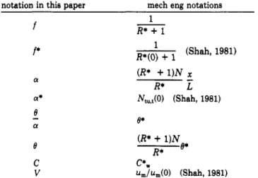
1981) is quite different from that used here. To facilitate the conversion to the nomenclature used in mechanical

engineering publications, a table for conversion is provided

in Table 111.

Summary and Conclusions

In this paper, we have presented approximate solutions for the transient response of shell and tube heat exchangers. These solutions are obtained from the exact solutions in our previous publication. It has been shown that the limiting "no wall" solutions can be deduced from the ap-

proximate solution for small values of Cf. For the response

Table 111. Table for Conversion to Mechanical Engineering

Notation

notation in this paper mech ena notations

f f* a a* 0

-

a e C V 1 R*

+

1 (Shah, 1981) 1 R*(O)

+

1

e*

(R*

+

l)N

R*

c*w

e*

u,/u,(O) (Shah, 1981) to shell fluid temperature change, the previous published

analytic solution for large values of

C

(Myers et al., 1970)

is also directly derivable from the exact solution. Rizika's

(1956) analytic solution in terms of hyperbolic functions was shown to be identical with the first three terms of eq

1. The case off = 1 for which London et al. (1959) gave

an exact solution can also be derived starting with our

(6)

1644 Ind. Eng. Chem. Res., Vol. 30, No. 7,1991

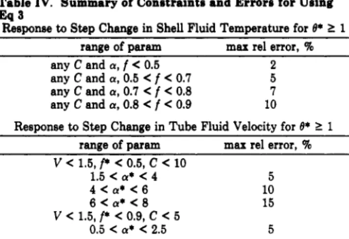
Table IV. Summary of Constraints and Errors for Using

Response to Step Change in Shell Fluid Temperature for 8* 2 1

Eq 3 range of param any C and a, f C 0.5 any C and a, 0.5 C f C 0.7 any C and a, 0.7 < f < 0.8 any C and a, 0.8 C f C 0.9

max re1 error, %

2 5

7

10

Response to Step Change in Tube Fluid Velocity for 8* 1 1

range of D B T B ~ max re1 error, %

V C 1.5, f* C 0.5, C C 10 1.5 C a* C 4 5 4 C a * < 6 10 6 < a * C 8 15 0.5 < a* < 2.5 5 V C 1.5, f* C 0.9, C < 5

=

Pw.

It is noted that the previously derived exact solu-

tions and the approximate solutions presented here are

also

applicable to crosscurrent, cocurrent, or countercurrent flow heat exchangers with an infiite capacitance rate fluid. In the previous paper (Tan and Spinner, 1978) and in

this

work it has been found that neglecting the $-function

term in the exact solution leads to small error for C

<

5

and a

>

2. Thus the exact solution without the $ function provides a good approximation for many practical values

of C and a. Thus only tabulated values of the known

mathematical function J or +1 in addition to the expo-

nential terms will be required for the numerical evaluation

of the transient response. For engineering design calcu-

lations, it is desirable to use a simple form of equation. Thus we have formulated a simple exponential form of

equation for approximating the transient response. It is

noted that the constant present in the exponential form

of equations is obtained by matching the slope of the re-

sponse curve of the exact solutions. Hence the resulting

approximate solutions are not entirely empirical. For the

response to shell fluid temperature, the exponential ap-

proximate solution gave excellent agreement with the exact solution for any values of C and a, except for f

>

0.5. For

the response to tube

fluid

velocity change, the approximate

exponential form of solution resulted in at most 5% relative error if 1

<

a*

<

4, f*

<

0.5,

C

<

10, and

V

<

1.5. Table IV summarizes the range of constraints and the maximum relative error for the use of eq 3. A further

practical use of this exponential form of approximate so-

lution is the estimation of the time required to reach a given fractional attainment of final steady state given the

magnitude of C, f, and a. In addition, it can be easily

adopted for the study of the dynamic response to time- dependent disturbances.

Nomenclature

C = thermal capacity ratio of tube wall to tube fluid, di-

mensionless

C* = thermal capacitance rate ratio of

ch/c,,

dimensionless

Ch = thermal capacitance rate of hot fluid, W/"C

C,

= thermal capacitance rate of cold fluid, W/"C

P

= initial fractional heat-transfer resistance on the shell side

f = final fractional heat-transfer resistance on the shell side

H = Heavieide function with H(O*<l) = 0 and H(O*ll) = 1

Io

= modified Bessel function of the first kind of order zero

J = mathematical function, defined in the text

L = heat exchanger flow length, m

rt = exponent in velocity-dependence heat-transfer correlation

N

= number of heat-transfer unite, dimensionless

R*

= ratio of fluid heat-transfer resistance of C, and Ch fluid

P = normalized final steady state tube fluid temperature,

equation

dimensionless

U

= fractional attainment of final steady state

Vl = fractional attainment of fiial steady state at 8* = 1

V = normalized linear velocity of tube fluid, dimensionless

x = length coordinate in flow direction, m

Greek Letters

CY = normalized exchanger length variable, dimensionless

8 = normalized time variable, dimensionless

8* = normalized throughput time, dimensionless

4,, = mathematical function, defined in text

+1 = mathematical function = 1 - J , defined in text

fi = mathematical function, defined in text

Appendix 1. Evaluation of Time Derivative from Exact Solution for Response to Step Change in

Shell Fluid Temperature For

e*

<

1 [exp(-R2aB*)

-

e x p ( - R l a 8 * ) ] ~

au

RlR2

ae*

R~ - R~

T-

- = - For

e*

1 1

(7)

Nota that _{The relationships o f f}and f c , a and a* are

P a *

f*v” a=-

f = 1 + ( v “ - l ) f C 9 V

- -

a’

-

[AR,

exp(-R2a8*)

-

BR3 exp(-R1d*)]-

Evaluation of Time Derivatives. For 8*

<

1 1

ae*

P

For

e*

1 1

1

au

ae*

-

[AR4 exp(-R2a8*)

-

BR, exp(-RlaO*)]- It”

+

_ -

Thus we have shown that

Appendix 2. Exact Solution for Response to Step Change in Tube Fluid Velocity and Evaluation of Its Time Derivatives

Exact Solution for Response to Step Flow Rate Change.

U

=

L(

1

-

A exp(-R,aO*)

+

B exp(-R3aO*)

+

H(B* -

P

1)B exp -R3a

+

(

CfR3

-

1 -

(&

- R3)(0* - l)a]g[ ( R ~

-

&)(e*

- u a ,

-

[(6-

H(e*

-

1)A exp(-R4a8*)dl R4)(0*

-

l ) a ,

1) exp[-(l- f ) a

+

(1

-

f*)a*l41

[

(e*

fa]) where

“1

+

[

1

+

6 -

(1 - 1 R3

’[

[

1

+

cf

-

(1

-

f*)- 2

v”

2

4

1 -

;[

1

-

f

-

(1 - f * ) q l i 2 ]

v”

“1

-

[ [

1

+

$

- (1 - 1 R 4 =

’[

[

1

+

q -

(1 -f c ) - 2

v”

P ) 3 -

;[

1

-

f

-

(1

-r)”l11’2]

v” 1 R , > - > R 4 > 0 f o r V < l R3

>

-

>

0

>

R4 for

V >

1

The two velocity forcing functions are Cf

Cf

1

F 1 = - -

v” V 1, Fz =

($

-

1)/C

The normalized final steady state is

T“

= 1

-

exp[-(1

-

n a

+

(1

-

P)a*]. For 8*

<

1 For 8* 2 1 a - [ A R 4 exp(-R,a)

-

BR3 exp(-R3a)]

+

“(

-

P

T”

Cf exp[-a

+

(1

-

fC)a*] a 1

= -[AR4 exp(-R4a)

-

BR3 exp(-R3a)]-

+

P

T”

$[A(

$

- R4)

+

g ( R 3 -

6)

-

$1

exp[-a

+

-

(1

-

f*)ff*l a = d [ A R 4 exp(-R4a)

-

BR3 exp(-Rga)]

+

(BR3

-

T”

AR4) exp[-a

+

(1

-

fC)ar*])

Note that

exp( -R4a -

*)

= ex,( -R3a

+

exp[-a

+

(1

-

fC)a*]

(8)

1646 I n d . Eng. Chem. Res. 1991,30,1646-1651

Literature Cited

Helfferich, F. Zon Exchange; McGraw-Hilk New York, 1962.

K a y , W. M.; London, A. L. Compact Heat Exchangers, 2nd ed.;

McGraw-Hilk New York, 1964.

London, A. L.; Biancardi, F. R.; Mitchell, J. W. The Transient Re-

sponse of Cas-Turbine-Plant Heat Exchangers-Regenerators, In- tercoolers, Precoolere, and Ducting. Trans. ASME J. Eng. Power, Series A 1959,81,433-448.

Myers, G . E.; Mitchell, J. W.; Lindeman, Jr., C. F. The Transient Response of Heat Exchangers Having An Infinite Capacitance Rate Fluid. Trans. ASME J . Heat Transfer 1970,92,269-275.

Rizika, J. W. Thermal Lags in Flowing Incompressible Fluid System.

Trans. ASME 1966, 78,1407-1413.

Shah, R. K. The Transient Response of Heat Exchangers. In Heat

Exchanger: Thermal-Hydraulic Fundamentals and Design; Ka-

kac, S., Bergles, A. D., Mayinger, F., Eds.; Hemisphere: Bristol,

PA, 1981; pp 721-763.

Sherwood, T. K.; Pigford, R. L.; Wilkes, C. R. Mass Transfer;

McGraw-Hill: New York, 1975.

Tan, K. S.; Spinner, I. H. Dynamics of A Shell-and-Tube Heat Ex- changer with Finite Tube-Wall Heat Capacity and Finite Shell- Side Resistance. Znd. Eng. Chem. Fundam. 1978, 17, 353-358.

Tan, K. S.; Spinner, I. H. Numerical Methods of Solutions for Con- tinuous Countercurrent Processes in the Nonsteady State, Part

I Model Equations and Development of Numerical Methods and Algorithms. AIChE J. 1984, 30, 770-779.

Received for reoiew August 15, 1990

Accepted August 28,1990

Dynamics of Fluid Mixing Induced at a T-Junction.

2.t

An Evaluation

of

a Mathematical Model with Existing Experimental Observations

S h a w

H.

Chen* and Jane

J. Ou

Department of Chemical Engineering, 206 Gavett Hall, University of Rochester, Rochester, New York 14627-0166

Alexander

J.

D u k a t

Columbia Gas System Service Corporation, 1600 Dublin Road, Columbus, Ohio 43216-2318

Mixing induced by flow through a T-junction is described with a mathematical model based on the

flow geometry comprising the jet trajectory, the evolution of the jet cross section, and the three- dimensional velocity distribution constructed for the jet stream. The experimentally determined

maximum tracer concentration across the main pipe reported in the literature is found to be closely

represented by the present model. The predicted second moment is also found to agree with the

existing correlation based on the integral analysis incorporating scaling laws and verified with extensive experimental observations.

I. Introduction

Flow through a T-junction has been considered a sen-

sible means to promote mixing, and hence heat and mass

transfer and chemical reaction (Kadotani and Goldstein,

1979; Forney and Kwon, 1979; Kim, 1985; Tosun, 1987). In the natural gas industry, effective utilization of a local production relies on mixing with a high-quality main stream via flow through a T-junction (Chen et al. (1990),

referred to hereafter as part 1). Conceptually, mixing is

caused by fluid flow that defines the fluid macroscale on which micromixing takes place via molecular diffusion. Thus, a problem involving mixing with simultaneous chemical and/or physical processes can be treated from a streamline perspective (e.g., Ou et al., 1985). Such an

approach has its general appeal to a problem in which the

underlying three-dimensional flow field could be established analytically or numerically from a fluid dynamic standpoint; laminar flow in a device with a simple geometry represents a manageable example (e.g., Lee et al.,

1987). Mixing induced at a T-junction, in which turbulent flow occurs within a rather complex geometry, remains a challenging problem for which a solution of a fundamental nature is attempted.

In the work reported here the flow geometry is syn- thesized through considerations of the jet trajectory as well

as the growth of the jet stream via entrainment

(Hill,

1972).

Mixing between the jet stream and the ambient fluid is

*

Author t o whom correspondence should be addressed.

'Part 1: Chen, 5. H.; Ou, J. J.; Dukat, A. J.; Murthy, J. Y. Id. Eng. Chem. Res. 1990,29, 1690-5.

Qs8s-5ss5/91/2630-1646$02.50/0

thus envisioned to occur through the jet entrainment of the ambient fluid as well as turbulent mass transfer across the jet/ambient boundary. One of the unique features of our approach is the new physical insight into the evolution

of the jet cross section that permits the three-dimensional

flow field to be established for the jet stream. The treatment of a jet stream staying in contact with the main pipe wall is the other unique feature of the present study. The mathematical model is tested by comparing the predicted values for both the maximum and the second moment of the tracer concentration distribution across the main pipe to the experimental observations reported by Forney and his co-workers (Forney and Kwon, 1979;

Forney and Lee, 1982; Sroka and Forney, 1989) over a wide

range of flow conditions. 11. Mathematical Model

In the model to be presented, a passive tracer is injected

as a side stream into a main flow containing no tracer. Both flow streams enter a T-junction at the same temperature, pressure, and essentially the same density for a relatively low tracer concentration. Flow conditions leading to both a free jet, defined here as a jet stream

staying clear of the main pipe wall, and a wall jet, Le., a

jet stream staying in contact with the main pipe wall, are considered; the geometric features of both cases are de-

picted in Figure l. Moreover, the jet-to-ambient flow

velocity ratio

R,

uj,/u, will be varied from 0.05 to 7,

which covers a wide range of conditions, to permit the present model to be tested with existing experimental results for T-mixing (Forney and Kwon, 1979; Forney and