Reducing the Variation of Gene Expression Patterns: A Grey Model Approach Applied to Microarray Data Classification

全文

(1)Int. Computer Symposium, Dec. 15-17, 2004, Taipei, Taiwan.. Reducing the Variation of Gene Expression Patterns: A Grey Model Approach Applied to Microarray Data Classification Tsun-Chen Lin1, Ru-Sheng Liu2, Chen-Chung Liu3, Shu-Yuan Chen4 Department of Computer Science and Engineering, Yuan Ze University 1 lintsunc@ms01.dahan.edu.tw, 2 csrobinl@saturn.yzu.edu.tw 3 christia@saturn.yzu.edu.tw, 4cschen@saturn.yzu.edu.tw Chieh-Yu Chen Graduate School of Biotechnology and Bioinformatics, Yuan Ze University cychen@mars.csie.ntu.edu.tw Abstract The gene expression levels measured from microarray spots vary between patients with the same type of tumor. This reduces the performance of microarray classification, especially when the microarray dataset has few samples. Here, we introduce the grey model GM(1,1) of the grey system theory for modeling gene expression patterns of small samples to eliminate variations. To evaluate the application of GM(1,1), we have combined GM(1,1) with GA/MLHD approach to solve the problem of multi-class classification. The GM(1,1)GA/MLHD model was tested on two published microarray datasets: (1) NCI60 cancer cell lines and (2) the GCM dataset. The experimental results show that the GM(1,1) gave gene expression patterns with less variations and helped the MLHD classifier to improve classification accuracy over the method of GA/MLHD, but they also outperformed many class prediction approaches.. Keywords: GM(1,1), microarray, genetic algorithm, classification, tumor class.. 1. Introduction The development of microarray technologies has provided a powerful tool by which the expression profiles of thousands of genes can be monitored simultaneously. One of the most promising applications of this technology is to provide a useful tool for tumor classification. Several previous works such as Alizadeh et al. [1], Ben-Dor et al. [2], and Golub et al. [14] have been proposed and have given promising results for most binary class data. However, if we consider the classification of gene expression data into more than two classes, the performance of most binary or 3-class methods will decrease significantly. One of the reasons is that a dataset may. contain many classes and the sample size is small. Recently, Romualdi et al. [5] tried a simulation approach to control the huge source of variation among and between patients and to evaluate a series of supervised statistical techniques. The simulation results show that all the methodologies have comparable performances when the number of patient samples per tumor is greater than 50, the number of tumors is lower than 4 and the number of discriminating gene is larger than 40. As there might be over a hundred types of cancer and potentially even more subtypes Hanahan. and Weinberg. [6] the microarray experiments are still too costly and time consuming so limit the number of samples, and therefore make variations within a class become more accentuated relatively. This fact suggests that the methodologies used to reduce the variability of gene expression patterns should be encouraged for practical applications. The grey model GM(1,1) as introduced by Deng. [8-9] has been successfully used in many research areas to filter out the random variations in control systems. This leads to our proposal for using GM(1,1) to reduce the variability and identify regularity of gene expressions. The key issues in using GM(1,1) are based on the accumulated generating operation (AGO), a group of differential equations, and the inverse accumulated generating operation (IAGO) to transform gene expression profiles. In this work, we have made many experiments using the GM(1,1)GA/MLHD (genetic algorithm/maximum likelihood) approach of Ooi et al. [3] under different parameter settings of GA in order to demonstrate that GM(1,1) has generality to take the advantage not only of transforming a gene expression pattern into a lessnoise pattern by using a few samples (at least 4 samples /class), but also of assessing the regularity for patterns to associate their phenotypes unique to a class. Finally, our method provides an average 2.5% improvement in classification accuracy for NCI60 data, and 2% improvement for the GCM dataset. In. 1198.

(2) Int. Computer Symposium, Dec. 15-17, 2004, Taipei, Taiwan.. addition, the importance of gene selection on microarray data analysis was also emphasized.. ˆ Y method by pseudo-inverse matrix B  applied and yields. is. a T 1 ˆ   ( B B ) BY u . 2. Methods 2.1. Data Transformation of GM(1,1) GM(1,1) is one of the GM(m,n) models of grey system theory. The m=1 and n=1 inside the parentheses indicate the 1st-order AGO and the number of variables of the differential equation, respectively. Our works, following the GM(1,1) model, would initially treat a given gene expression pattern of uncertain (high or low) expression values as a serial output of a variable/gene from different patients with the same type of tumor. When constructing a grey model, the GM(1,1) first applies a 1st-order AGO to this pattern to provide the middle message to weaken the variation tendency. Next, a group of grey differential equations were used to give function to this AGO-generated gene expression pattern. Finally, the GM(1,1) requested a 1st-order IAGO (Inverse-AGO) to predict the outputs of gene expressions from GM(1,1)-treated sequence. Therefore, the proposed method is composed of the operations: AGO, GM(1,1), and IAGO for the purpose of transferring raw gene expressions to a new gene expression pattern by steps described in detail as follows. Step 1. Let y i( 0 ) be the gene expression levels for a given gene i to a specific tumor type. yi( 0) ( yi( 0) (1), yi( 0) ( 2),......., yi( 0) ( k )), k 4. where. (0) (1) yˆ ( k ) yˆi(1) ( k ) yˆ (4) i i ( k 1) Equation (5) is calculated by substituting Equation ( 0) (3) into Equation (4) so that the yˆ with respect to i ( 0) the data sequence yi is obtained by. u  ( 0) ( 0) yˆ y i (1)    (1 e a )  e a ( k 1) (5) i ( k )  a   Step 5. Following the method mentioned above, a dataset then can be preprocessed by following procedures to filter out the noises and will be used by the classifier. 1. 2. 3. 4.. k. y. (0) i (. 2.2. Reviews of GA/MLHD. The number “ 1”in the parentheses on the superscript denotes 1st-order AGO. Step 3. To derive the exponential 1st-order grey function of y i(1) , the GM(1,1) defines the grey differential equation as. y i(0) ( k ) az i(1) ( k ) u (1) where a is the development coefficient and u is the grey control variable of GM(1,1). We also define. zi(1) (k) ( yi(1) (k) yi(1) (k 1)),k 2,3,.....n where the parameter =0.5 means a MEAN operation on y i(1) . Next, we can build up the whitening equation corresponding to Equation (1) as ay i(1) (k ) u. For each class Cj in gene expression profiles For each gene i in gene expression profiles For each sample’ s order k1 in Cj Calculate Equation (5). j ), k 1, 2 ,.... n. j 1. dy i(1) (k ). 1 y i( 0 ) ( 2 )   (0)   1 y (3)  ..  Y  i  .. .    .     (0)  1 y ( n )  i . (1) Substituting a and u into Equation (2), the yˆ i (k) can be obtained and further be expressed as u  a ( k 1) u  (0) (1) yˆ y i (1)   e  (3) i ( k )  a a  where the symbol “ ^”means the prediction value. ( 0) (1) Step 4. To predict sequence yˆ from yˆ , the i i corresponding IAGO is defined as. where k denotes the number of samples. Step 2. To reduce the variations, we define the 1storder AGO on y i( 0 ) by following operation. y i(1) ( k ) AGO y i( 0 ) .  z i(1) (2)  (1) z i (3)  B  . .  . (1)  z i (n) . (2) dx For an approximate solution to determine the a and u of Equation (1), the least squares estimation. Examinations to the GM(1,1) model, applied to microarray classification, were performed by using an available implementation of the GA toolbox for gene selection and the MLHD classifier for discrimination analysis from Ooi et al. [3]. In order to work with an ensemble of different gene subspaces (sets of predictor genes), this GA toolbox provides two selection methods: (1) stochastic universal sampling (SUS) and (2) roulette wheel selection (RWS). It also provides two tuning parameters, Pc: crossover rate and Pm: mutation rate, used to tune one-point and uniform crossover operations to evolve the population in the mating pool for choosing the optimal genes, consisting of chromosomes, to work with the MLHD classifier. For the discrimination analysis to a chromosome, the chromosome is designed by a string Si, Si = [R g1, g2… gi=Rmax], where R value denotes the number of genes, and g1, g2…gi=Rmax denotes the indices of. 1199.

(3) Int. Computer Symposium, Dec. 15-17, 2004, Taipei, Taiwan.. predictor genes. In the process of pattern classification, the first R genes out of g1, g2… gi=Rmax are then used to form dataset of sample patterns for all samples and will be fed into the MLHD classifier. The essence of the MLHD classifier is based on a discriminant function to estimate the discrimination score of genes in classifying tumor samples, and it is given by    1   f q (e ) qT 1 e  qT 1 q 2  T where  is the class mean q (  q ,1 ,  q , 2 .... q, R ) vector, q,i is the average expression level of gene i for all samples belonging to class q,  means the common covariance matrix [10] between classes and is defined as Q 1  q M t Q q 1. where q , q{ 1, 2, ……, Q} is the class covariance matrix of the selected R genes for all training samples belonging to class q, and Mt is the number of all training samples. To predict the class of an query sample  pattern e (e1 , e2 ,....., eR )T  class q, where the element ei is the expression level of gene i, the classification rule of the MLHD classifier is defined as    C( e ) = q, where f q (e ) f r (e ) (6) for q r , r{ 1, 2…Q} ,a n dQ is the possible classes of the experiment dataset. The MLHD classifier also defines a fitness function as f (Si) = 200 –(EC + EI), where EC is the error rate of the Leave-One-Out Cross-Validation (LOOCV) test on the training data , and EI is the error rate of independent test on the test data. By calculating Ec and Ei under the classification rule as Equation (6), the returning fitness value, which is in turn, will be used by GA to evolve better gene subsets.. dataset of reduced dimensions and to be evaluated by MLHD classifier. 1. FOR each generation G=1 to G=100 2. FOR each chromosome C=1 to C=100  3. FOR each training sample e class q 4. Build up discriminant model with remaining training samples for LOOCV tests   5. IF ( f q (e ) f r (e ) ) 6. XcError = XcError + 1 // sample misclassified 7. END FOR  8. FOR each unknown sample e class q 9. Build up discriminant model with all training samples for independent tests   10. IF ( f q (e ) f r (e ) ) 11. XiError = XiError + 1 // sample misclassified 12. END FOR 13. EcErrorRate = XcError / Total training samples 14. EiErrorRate = XiError / Total test samples 15. Fitness[G][C]=200–(EcErrorRate + EiErrorRate) 16. END FOR 17. END FOR 18. Findmax (Fitness ) // best chromosome In the running of above program through 100 generations and 100 individual runs, the chromosome with the best fitness, chosen from the simulation to arrive at the optimal operation will be based on the idea that a classifier need not only work well on the training samples, but also work equally well on previously unseen samples. Therefore, the optimal individuals of each generation were sorted in ascending order by the sum of the error number on both tests. The smallest number then determines the chromosome that contains discriminatory genes and the number of genes needed in the classification as well as gives the classification accuracy obtained by our methods.. 3. Datasets 2.3. Prediction Errors In a domain of Q classes, the success rate estimations through GM(1,1)-GA/MLHD method begin with setting 100 runs by following the program, with each run beginning with a different initial gene pool in order to have an unbiased estimate of classifier performance. The maximum generations for each run are set to 100, which each generation produces 100 and 30 chromosomes with size of genes ranging from Rmin=11 to Rmax=15 and from Rmin=5 to Rmax=50 in a chromosome corresponding to the NCI60 and the GCM dataset respectively. According to the gene indices in each chromosome, only the first R numbers of genes out of g1, g2,… gnmax are picked to form sample patterns for all samples and hereby assume that we are given a. There are two published microarray datasets from human cancer cell lines will be used in this paper. Before the datasets were used in our experiments, the data was preprocessed by following steps. 1. The spots with missing data, control, and empty spots were excluded. 2. For each sample array in both datasets, the gene expression intensity of every spot was normalized by subtracting the mean expression intensity of control spots and dividing the result by the standard deviation of control spots. 3. A preliminary selection of 1000 genes with the highest ratios of their between-groups to within– groups sum of squares (BSS/WSS) was performed. In our case, the BSS/WSS ratios for NCI60 data are ranging from 0.4 to 2.613 and from 0.977 to 3.809. 1200.

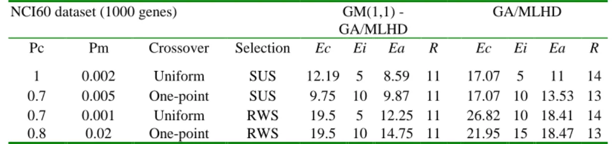
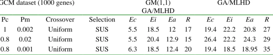
(4) Int. Computer Symposium, Dec. 15-17, 2004, Taipei, Taiwan.. for the GCM. For gene i, xij denotes the expression level from patient j, and the ratio is define as Mt. Q. I (c. j. q)(qi i ) 2. I (c. q)( xij qi )2. BSS (i ) j 1 q 1  Mt Q WSS (i ). j 1 q 1. j. where Mt is the training sample size, Q is the number of classes and I(• ) is the indicator function which equal 1 if the argument inside the parentheses is true, and 0 otherwise. •i denotes the average expression level of gene i across all samples, qi denotes the average expression level of gene i across all samples belonging to class q. This is the same gene preselection method as the paper of Dudoit et al [12].. The GCM dataset Ramaswamy et al. [14] were measured by Affymetrix Genechips containing 16063 genes among 198 samples with 14 different classes of tumor, and can be obtained from http://wwwgenome.wi.mit.edu/mpr/publications/projects/Global _Cancer_Map/. In our data preprocessing, the dataset left a matrix of 1000 genes 198 samples. These genes are referred to by their index numbers (1 to 1000) in our experiments. This dataset originally contains 144 samples for training, and 54 for testing. The 144 patient samples are gene expression levels composed of 8 breast, 8 prostate, 8 lung, 8 colorectal, 16 lymphoma, 8 bladder, 8 melanoma, 8 uterine, 24 leukemia, 8 renal, 8 pancreatic, 8 ovarian, 8 mesothelioma, and 8 brain.. 4. Results and Discussions. 3.1. The NCI60 Dataset. 4.1. Classification Accuracy. The NCI60 dataset Ross et al. [7] were measured with 9,703 spotted cDNA sequences among the 64 cell lines from tumors with 9 different sites of origin from the National Cancer Institute’ s anti-cancer drug screen and can be downloaded from http://genomewww.stanford.edu/sutech/download/nci60/dross_arra y_nci60.tgz. During the data preprocessing, the single unknown cell line and two prostate cell lines were excluded due to their small sample size, leaving a matrix of 1000 genes 61 samples. These genes are henceafter referred to by their index numbers (1 to 1000) in our experiments. To build the classifier and run GM(1,1) in a small size of training samples, this dataset was divided into a learning and test set (2:1 scheme, 41 samples for training and 20 for testing). The 41 patient samples are gene expression levels composed of 5 breast, 4 central nervous system (CNS), 5 colon, 4 leukemia, 5 melanoma, 6 nonsmall-cell-lung-carcinoma (NSCLC), 4 ovarian, 5 renal, and 3 reproductive.. In this section, the classification accuracy of MLHD classifier, using GM(1,1)-treated NCI60 dataset, will be compared to its performance without using GM(1,1)-treated data. From Table 1, the best predictive accuracies are achieved using the Uniform crossover and SUS selection strategy with GAs. The best predictor set obtained from GM(1,1)-GA/MLHD method exhibits a cross-validation success rate of 87.8% while the success rate of GA/MLHD is 83%. Even in diagnosing blind test samples our method needs only 11 predictive genes to produce a success rate of 95% (overall success rate = 91.4%), whereas GA/MLHD needs 14 predictive genes to produce Ei = 95% (overall success rate = 89%). If we take only the average performance over different parameter settings on independent test data, the mean test error rate in the model of GM(1,1)-GA/MLHD is 7.5%, and in the model of GA/MLHD it is 10%. This indicates that our method is better than GA/MLHD and has improved 2.5% better classification accuracy.. 3.2. The GCM Dataset Table 1. Recognition error rate (%) and the parameters used in the NCI60 dataset. NCI60 dataset (1000 genes) GM(1,1) GA/MLHD GA/MLHD Pc Pm Crossover Selection Ec Ei Ea R Ec Ei Ea R 1 0.7 0.7 0.8. 0.002 Uniform SUS 12.19 5 8.59 11 17.07 5 11 0.005 One-point SUS 9.75 10 9.87 11 17.07 10 13.53 0.001 Uniform RWS 19.5 5 12.25 11 26.82 10 18.41 0.02 One-point RWS 19.5 10 14.75 11 21.95 15 18.47 Ea: overall error rate ((Ec + Ei) / 2); R: optimal number of predictive genes.. Having obtained good performance on the NCI60 dataset with 9 classes, we next tested the proposed method on a more complicated dataset consisting of 14 classes with each class containing more samples to examine the generality of our method. By using the experience with the NCI60. 14 13 14 13. dataset, we also employed the Uniform and SUS strategies and set the Pc = 1, 0.8, 0.8, and Pm = 0.002, 0.02, 0.001 respectively. From Table 2, the best outcomes that selected an optimal gene set of 17 elements producing Ec = 5.5% and Ei = 18.5% (over all rate = 12%) of our method still outperformed. 1201.

(5) Int. Computer Symposium, Dec. 15-17, 2004, Taipei, Taiwan.. GA/MLHD method, which selected an optimal geneset of 35 elements, producing Ec = 19.4% and Ei = 18.5% (over all rate = 18.95%). When the NCI60 and the GCM datasets have become two popular benchmark data used by many classification algorithms, we list the performance differences for the NCI60 and the GCM datasets among various. methods. More detailed discussions to these methods can be found in the papers of Ooi et al. [3], Yeang et al. [4], and Peng et al. [13]. In our comparisons with these methods, we found the best model of our methods yielded clear improvements compared to other approaches listed in the Table 3 with respect to the dataset they used.. Table 2. Recognition error rate (%) and the parameters used in the GCM dataset. GCM dataset (1000 genes) GM(1,1) GA/MLHD GA/MLHD Pc Pm Crossover Selection Ec Ei Ea R Ec Ei Ea R 1 0.002 Uniform SUS 5.5 18.5 12 17 19.4 22.2 20.8 27 0.8 0.02 Uniform SUS 5.5 20.4 12.9 15 26.4 22.2 24.3 29 0.8 0.001 Uniform SUS 6.3 18.5 12.4 20 19.4 18.5 18.95 35 Ea: overall error rate ((Ec + Ei) / 2); R: optimal number of predictive genes. Table 3. Classification accuracy comparisons among different approaches. LOOCV Independent Overall Genes Reference NCI 60 dataset (%) test (%) (%) needed GM(1,1)-GA/MLHD 88 95 92 11 [This paper] GA/MLHD 83 95 89 14 [3] GA/SVM/RFE 88 －－ 27 [13] GCM dataset GM(1,1)-GA/MLHD GA/SVM/RFE GA/MLHD OVA/SVM OVA/KNN. 94 85 79 81 73. 82 － 82 78 54. 4.2. Perturbed Versions of Learning Data In this section, we examine a possible effect that may influence the tumor classification using the GM(1,1) model. As we have mentioned, for a given gene, GM(1,1) generated new pattern, which was transformed from the original gene expression levels across a set of micrarrays through Equation (5) depending on the development coefficient, the grey control variable and the first value of the original sequence. We questioned whether if we reorder the order of input sequence, GM(1,1) may be capable of selecting better patterns for discrimination analyses. Therefore, we took the NCI60 dataset for example and tried to randomly reorder the learning dataset. 88 － 82 80 63. 17 26 32 16063 100. [This paper] [13] [3] [4] [4]. into 30 different perturbed versions of the same size as the original learning set without changing the test data in order to examine the effect of sequence order on the results of classification. Strikingly, with the Uniform and SUS strategy of GA, we found that the best version of training dataset produced a crossvalidation error rate equal to 2.4% and a test error rate equal to 5%. In Table 5, we list the results performed by the best and worst versions of the datasets, as well as the average performances over 30 learning sets. Although this procedure is computationally more expensive, it is valuable for the pattern recognition to select discriminatory genes and thus improve the accuracy in the classification.. Table 5. Classification results of 30 different training sets for the NCI60 data. NCI60 dataset (1000 genes) Best Worst Average Pc Pm Crossover Selection Ec Ei Ea R Ec Ei Ea R Ec Ei Ea R 1 0.002 Uniform SUS 2.4 5 3.7 11 12.2 5 8.6 13 2.6 5.7 4.15 11 Ea: overall error rate ((Ec + Ei) / 2); R: optimal number of predictive genes.. 1202.

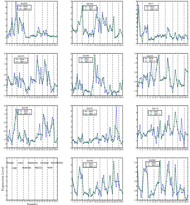
(6) Int. Computer Symposium, Dec. 15-17, 2004, Taipei, Taiwan.. 4.3. Gene Expression Patterns According to the assumption of Yeang et al. [4], individual genes for the same type of tumor may share some expression profile patterns unique to their class. The usage of GM(1,1) to provide gene expression profiles with less variations within a class but more discriminatory information among classes then will help gene expression patterns catch internal regularity and become more tightly associated to class phenotype for samples in the same tumor class. Figure 1 illustrates 11 discriminatory gene patterns 10. 5. Gid:539 RAW GM(1,1). 8. 4. 6. 3. 4. 2. 2. 1. 0. 0. -2. -1. indexed by 539, 493, 11, 470, 460, 975, 326, 341, 112, 626, 996 corresponding to the NCI60 training dataset, and compared to original gene expression patterns. Clearly, the GM(1,1) method inflates the variance of observations and hence assess the smaller variability within a class. This is the reason why GM(1,1) is useful to form gene patterns as good candidates for molecular fingerprints in tumor classification. And we also believe that classification methods, by carefully choosing predictor genes used by a classifier from better quality gene expression patterns, will thus help classification analysis.. GID:493 RAW GM(1,1). 8 7 6. Gid:11 RAW GM(1,1). 5 4 3. -4. 1 3 5 7 9 11 13 15 17 19 21 23 25 27 29 31 33 35 37 39 41. 2.5. 6. Gid:470. 2. RAW GM(1,1). 1.5. -2. 5. 2 1 0 -1 1 3 5 7 9 11 13 15 17 19 21 23 25 27 29 31 33 35 37 39 41. 2.5. Gid:460 RAW GM(1,1). 4. 1. -1.5. -1. 0. 1 3 5 7 9 11 13 15 17 19 21 23 25 27 29 31 33 35 37 39 41. RAW GM(1,1). 1.5. -1. 6. Gid:326. 2. 5 4. 1. -1.5 1 3 5 7 9 11 13 15 17 19 21 23 25 27 29 31 33 35 37 39 41. Gid:341 RAW GM(1,1). 0. 2. -0.5. 1. -1. -2. 1 3 5 7 9 11 13 15 17 19 21 23 25 27 29 31 33 35 37 39 41. 4 Gid:112 3. RAW GM(1,1). 2. 3. 0.5. 1 0. 0. -1.5. -1. -1. -2 1 3 5 7 9 11 13 15 17 19 21 23 25 27 29 31 33 35 37 39 41. 3. -2. 1 3 5 7 9 11 13 15 17 19 21 23 25 27 29 31 33 35 37 39 41. 4. 4. Expression Level. -0.5. 1. 2.5. -2.5. 0. 2. -1. 1.5. Gid:975 RAW GM(1,1). 0.5. 0.5. -0.5. 2. 1 3 5 7 9 11 13 15 17 19 21 23 25 27 29 31 33 35 37 39 41. 1. 3. 0. -2. breast. 2. colon. CNS. melanoma. leukemia. bovarian reproductive. NSCCL. renal. 3 Gid:626. 3. RAW GM(1,1). 2. 1. 0.5. 0. 0 -0.5. -3. -1. -4 -5. 1. 3. 5. 7. 9 11 13 15 17 19 21 23 25 27 29 31 33 35 37 39 41. Samples. -2. 2. Gid:996 RAW GM(1,1). 1. 1. -2. 2.5. 1 3 5 7 9 11 13 15 17 19 21 23 25 27 29 31 33 35 37 39 41. 1.5. 0 -1. -2. -1 1 3 5 7 9 11 13 15 17 19 21 23 25 27 29 31 33 35 37 39 41. -1.5. 1 3 5 7 9 11 13 15 17 19 21 23 25 27 29 31 33 35 37 39 41. Figure 1. shows 11 gene expression patterns of the best predictor set selected fromt the GM(1,1)-GA/MLHD method and compares to original gene expression patterns. These patterns are gene expression levels composed of 41 samples: 5 breast, 4 central nervous system (CNS), 5 colon, 4 leukemia, 5 melanoma, 6 non-small-cell-lung-carcinoma (NSCLC), 4 ovarian, 5 renal, and 3 reproductive.. 1203.

(7) Int. Computer Symposium, Dec. 15-17, 2004, Taipei, Taiwan.. 5. Conclusions To obtain the ability to eliminate the variations in microarray data and find genetic fingerprints among various tumor classes, we propose using the GM(1,1)-GA/MLHD method for the classification problem of small-sample issues. Based on the success of our method, we conclude the main advantages of GM(1,1). First, GM(1,1) has the ability to smooth data variation by processing discrete numerical data into a pattern with less-noise, while the data in a class are not necessarily distributed normally. Secondly, the GM(1,1), representing a gene expression pattern shared by samples of the same tumor type, only needs a few samples to obtain better gene expression pattern. This is a reversal of traditional data mining techniques, where there are typically more samples than variables. The work reported here is an expansion of paper Ooi et al. [3]. Our approach combined GM(1,1) and GA/MLHD methods, using the same procedures in classification on the same dataset, and exhibiting a 2.5-4% improvement in accuracy. In the multi-class classification scenario, the currently available datasets containing relatively few samples but a large number of variables make it difficult to demonstrate one method’ s superiority. While no methods have yet become the standard method to be adopted in this domain, we have shown GM(1,1)-treated gene expression patterns along with classifiers outperform classifiers without GM(1,1)’ s. And finally, we anticipate that the use of GM(1,1) would be a helpful tool leading to practical uses of microarray data in cancer diagnosis.. [6] [7]. [8]. [9]. [10] [11]. [12]. [13]. References [1] A.A. Alizadeh, M.B. Eisen, R.E. Davis, C. Ma, I.S. Lossos, A. Rosenwald, J.C. Boldrick, H. Sabet, T. Tran, X. Yu, “ Distinct types of diffuse large B-cell lymphoma identified by gene expression profiling,”Nature, 403, pp.503–511, 2000. [2] A. Ben-Dor, N. Friedman, and Z. Yakhini, “ Scoring genes for relevance,”Technical Report AGL-2000-13 Agilent Laboratories, 2000. [3] C.H. Ooi, and P. Tan, “ Genetic algorithms applied to multi-class prediction for the analysis of gene expression data,”Bioinformatics, 19, pp.37–44, 2003. [4] C.H. Yeang, S. Ramaswamy, P. Tamayo, S. Mukherjee, R.M. Rifkin, M. Angelo, M. Reich, E.S. Lander, J.P. Mesirov and T.R Golub, “ Molecular classification of multiple tumor types,”Bioinformatics, 17, pp.S316–S322, 2001. [5] C. Romualdi, S. Campanaro, D. Campagna, B. Celegato, N. Cannata, S. Toppo, G. Valle, and G, Lanfranchi, “ Pattern recognition in gene. [14]. 1204. expression profiling using DNA array: a comparative study of different statistical methods applied to cancer classification,” Human Molecular Genetics, vol. 12, No. 8, pp.823-836, 2003. D. Hanahan, and R. Weinberg, “ The hallmark of cancer,”Cell, 100, pp.57–71, 2000. D.T. Ross, U. Scherf, M.B. Eisen,, C.M. Perou, C. Rees, P. Spellman, V. Iyer, S.S. Jeffrey, M.V. de Rijn, M. Waltham, A. Pergamenschikov, J.C. Lee, D. Lashkari, D. Shalon, T.G. Myers, J.N. Weinstein, D. Botstein, and P. O. Brown, “ Systematic variation in gene expression patterns in human cancer cell lines,”Nat. Genet, 24, pp.227–235, 2000. J.L. Deng, “ Control problems of grey system,” System and Control Letters, 5, pp.288-294, 1982. J.L. Deng, “ Introduction to Grey System Theory,”Journal of Grey System, vol.1, pp.1-24, 1989. M. James, “ Classification Algorithms,”Wiley, New York, 1985. S. Ramaswamy, P. Tamayo, R. Rifkin, S. Mukherjee, C. Yeang,, M. Angelo, C. Ladd, M. Reich,M, E. Latulippe, J. Mesirov, T. Poggio, et al., “ Multiclass cancer diagnosis using tumor gene expression signatures,”Proc. Natl. Acad. Sci USA, 98, pp.15149–15154, 2001. S. Dudoit, J. Fridly and T. Speed, “ Comparison of discrimination methods for the classification of tumors using gene expression data,”JASA, Berkeley Stat. Dept. Technical Report #576, 2000. S. Peng, Q. Xu, X. Ling, X. Peng, W. Du, L. Chen, “ Molecular classification of cancer types from microarray data using the combination of genetic algorithms and support vector machines,” FEBS Letters, 555, pp.358-362, 2003. T. Golub, D. Slonim, P. Tamayo, C. Huard, M. Gaasenbeek, J. Mesirov, H. Coller, M. Loh, J. Downing, M. Caligiuri, “ Molecular classification of cancer: class discovery and class prediction by gene expression monitoring,” Science, 286, pp.531–537, 1999..

(8)