模擬退火參數偵測系統於物件偵測與震測圖形之應用

(1)

模擬退火參數偵測系統於物件偵測與震測圖形之應用

Simulated Annealing Parameter Detection System for Object

Detection and Seismic Application

計畫編號：NSC 96-2221-E-009-197

執行期限：96 年 8 月 1 日至 97 年 7 月 31 日

主持人：黃國源交大資訊工程系 kyhuang@cis.nctu.edu.tw

一、中文摘要我們提出一個運用模擬退火演算法的參數偵測系統來偵測影像中的圓、橢圓，並以雙曲線的漸進線來偵測直線。在此系統中，我們定義了點到圖形的距離使得系統能夠成功的運作。這個模擬退火的參數偵測系統能找到一組圖形(圓、橢圓)的參數，使得影像上的點到這組圖形的距離為最小。除此之外，我們利用系統的誤差，或稱為能量作為判斷的依據來決定影像中圖形的數量。此系統對於影像中的直線、圓、橢圓均能成功的偵測。此結果將幫助影像中圖形的解釋，更可進一步應用於震測圖形的處理。關鍵詞：模擬退火、全域最佳化、類神經網路、Hough 轉換、震測圖形。 Abstract

Simulated annealing is adopted to detect the parameters of circles, ellipses, and detect lines as asymptote of hyperbolas in images and applied to seismic pattern detection. We define the distance from a point to a pattern such that the detection becomes feasible. The proposed simulated annealing parameter detection system has the capability of searching a set of parameter vectors with global minimal error with respect to the input data. Based on the error or energy, we propose a method to determine the number of patterns. Experiments on the detection of circles, ellipses, and lines as asymptotes of hyperbola in images are quite successful. The results can improve image interpretations and the system can be

applied to seismic signal processing in the future.

Keywords: simulated annealing, global

optimization, neural network, Hough transform, seismic pattern.

二、緣由與目的 近年來，類神經網路之研究在國內外受到相當的重視，其應用的領域更是相當廣泛，尤其是圖形識別上的應用。傳統上， Hough transform (HT) 曾經被應用在偵測參數圖形[1]-[2]，但是記憶體需求與峰值的偵測是其缺點。在2002、2003 年 J. Basak

和 A. Das 提出 Hough transform neural network (HTNN) 來偵測影像中的直線、圓與橢圓[3]-[4]，以改善這個問題。由於 HTNN 所採用的是梯度下降法 (gradient descent method) 來最小化點到圖形的距離，因此HTNN 有 local minimum 的問題。 1983 年，Kirkpatrick 等人提出的模擬

退火simulated annealing (SA) [5]這個全域

最佳化的方法，並且成功的運用在解決各種排列組合的問題上。在1987 年，Corana 等人成功的運用模擬退火的方法來解決連續函數的最佳化問題[6]。在此，我們便利用模擬退火的全域最佳化特性來解決 HTNN 會遭遇到的 local minimum 的問題，提出一個模擬退火的參數偵測系統來最小化點到圖形間的距離。我們首先給予每個圖形(直線、圓、橢圓)一組初始的參數。接著，對於每一個輸入點，計算點到每一個圖形的距離。然後計算點對所有圖形的總誤差值，並且利用模擬退火的方法來修正每個圖形的參數，

(2)

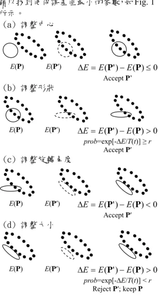
藉以找到使得誤差值最小的參數，如Fig. 1

所示。 _{system. The detection system takes the N}Fig. 2 shows the proposed detection data as the input, followed by the SA parameter detection system to detect a set of parameter vectors of K patterns. After convergence, K patterns are recovered from the detected parameter vectors.

(a) 調整中心 E(P) E(P′) _Δ_E ₌_E₍_P_'₎₋_E₍_P₎_≤₀ Accept P’ (b) 調整形狀 E(P) E(P′) _Δ_E₌_E₍_P_'₎₋_E₍_P₎_>₀ prob=exp[-∆E/T(t)] ≥ r Accept P′ (c) 調整旋轉角度 E(P) E(P′) _Δ_E₌_E₍_P_'₎₋_E₍_P₎_<₀ Accept P′ (d) 調整大小 E(P) E(P′) _Δ_E₌_E₍_P_'₎₋_E₍_P₎_>₀ prob=exp[-∆E/T(t)] < r Reject P′; keep P Fig. 1. Illustration of parameter learning.

SA parameter detection system consists of two main parts: 1. definition of system error (energy, distance); 2. SA algorithm for determination of the parameter vectors with minimum error. To obtain the system error, we calculate the error or the distance from a point to patterns, and combine the errors from all points to patterns to be the system error.

Any translated and rotated ellipse or hyperbola in 2D space can be expressed by the equation below:

f m y m x b m y m x a y x y x = − + − − + − + − 2 2 ] cos ) ( sin ) ( [ ] sin ) ( cos ) [( θ θ θ θ . (1) Table 1 lists the relation between a, b, f, and the graph. When an ellipse has the same a and b, the graph represents as a circle.

Table 1 Relation between graph and a, b, f in the equation.

三、結果與討論

(1) 結果:

(a) Simulated Annealing Parameter Detection System a b f Graph ＋＋＋ _Ellipse －－－ Ellipse ＋－ 0 Asymptote －＋ _{0 Asymptote}

The distance from a point xi = [xi yi]T to

the kth pattern is defined as Input

N data

Simulated annealing parameter detection system

Detected parameters Detected K patterns Fig. 2. The system overview.

. | ] cos ) ( sin ) ( [ ] sin ) ( cos ) [( | ) , ( 2 , , 2 , , k k y k i k x k i k k y k i k x k i k i i k f m y m x b m y m x a y x d − − + − − + − + − = θ θ θ θ (2)

When a point is on any pattern we have d(xi,

yi) = 0.

Error or distance from a point to the patterns is defined as the geometric mean of the distances from the point to all patterns. The error of the ith point xi is

(3)

[

_i _i _k _i _K _i

]

K i

i E d d d d

E = (x)= ₁(x) ₂(x )... (x)... (x ) 1 (3) Calculate the new energy E(P’) from N

points to K patterns. Using Metropolis criterion decides whether or not to accept

P′: If the new energy is less than or equal

to the original one, ∆E = E(P′) - E(P) ≤ 0, accept P′. Otherwise, the new energy is higher than the original one, ∆E = E(P′) - E(P) > 0. In this case, compute the probability prob = exp[-∆E/T(t)]. We generate a random number x uniformly distributed over (0, 1). If prob ≥ x, accept

P′; otherwise, reject it, and keep P.

where K is the total number of patterns. If the point is on any pattern, the error of this point will be zero.

The error or energy of the system is defined as the average of the error of points,

∑

= = N i i E N E 1 1 . (4) The simulated annealing algorithm to detect parameters is proposed below.

Algorithm: SA algorithm to detect

parameter vectors of K patterns including ellipses, circles, hyperbolas, and lines as asymptotes.

Input: N points in an image. Set K as the

number of patterns.

Output: A set of detected K parameter

vectors.

Step 1: Initialization.

In the initial step t = 1, choose T(1) = Tmax at high temperature, and define the

temperature decreasing function as T(t) = Tmax × 0.98(t-1)

Initialize parameter vectors, p1, p2, ...,

pk, …, pK, where pk = [mk,x, m k,y, ak, bk, θk,

fk]T, one p is for one pattern, and set P =

[p1, p2, ..., pk, …, pK].

Calculate energy E(P) as (2), (3), and (4). Step 2: Randomly change parameter vectors

and decide the new parameter vectors in the one temperature.

For m = 1 to Nt (Nt trials in a temperature)

For k = 1 to K (k is the index of the pattern)

Start a trial, including steps (a), (b), (c), and (d) in the following.

(a) Randomly change the center of the kth pattern:

(b) Randomly change the shape

parameters: n ab T k k T k k b a b a ' '] =[ ] +α [

and normalize it by |a_k'b_k |', where n = [n1 n2]Tis a 2 × 1 random vector, n1 and

n2 are Gaussian random variables with

N(0, 1) and αab is a constant. Now, pk′ =

[mk,x, mk,y, ak′, bk′, θk, fk]T, and P′ = [p1,

p2, …, pk′,…, pK].

Similar to Step 2(a), calculate the new energy E(P’) from N points to K patterns. Using Metropolis criterion decides whether or not to accept P’.

(c) Randomly change the angle: n

k

k θ αθ

θ' = +

where n is a Gaussian random variable with N(0, 1) and αθ is a constant. Here,

the angle is in degree. Now, pk′ = [mk,x,

mk,y, ak, bk, θk′, fk]T, and P′ = [p1, p2, …,

pk′,…, pK].

Similar to Step 2(a), calculate the new energy E(P′) from N points to K patterns. Using Metropolis criterion decides whether or not to accept P′.

(d) Randomly change the size: |

|

' f n

f _k= _k +α_f

where n is a Gaussian random variable with N(0, 1) and αf is a constant. Now, pk′

= [mk,x, mk,y, ak, bk, θk, fk′]T, and P′ = [p1, p2, …, pk′,…, pK]. n m T y k x k T k,y x k m' m m m' ] =[ ] +α [ _, _, _, where n = [n1 n2]T is a 2 × 1 random

vector, n1 and n2 are Gaussian random

variables with N(0, 1) and αm is a

constant. Now, p’k = [m’k,x, m’k,y, ak, bk,

θk, fk]T, and P′ = [p1, p2, …, p′k,…, pK].

Similar to Step 2(a), calculate the new energy E(P′) from N points to K patterns. Using Metropolis criterion decides

(4)

whether or not to accept P′. Table 2 Detected parameters in Fig. 3. End for k mx my a b θ f Ideal parameters 1st ellipse 25 25 2.5 0.4 10 121 2nd ellipse 30 30 2 0.5 0 64 Detected parameters 1st ellipse 25.3 24.6 2.4 0.4 11.8 118.8 2nd ellipse 30.0 34.9 2.1 0.5 0.2 64 End for m

Step 3: Cool the System.

Decrease temperature T according to the cooling function, T(t) = Tmax × 0.98(t-1),

for t = 1, 2, 3, …, to the next cooling cycle and repeat Step 2 and 3 until the temperature is low enough, for examples, repeat 500 times.

(b) Experimental Results

The detection system is applied to detect the lines, circles and ellipses in the image. The image size is 50×50. Each pattern has 50 points. Data are disturbed by Gaussian noise with zero mean and variance is 0.5,

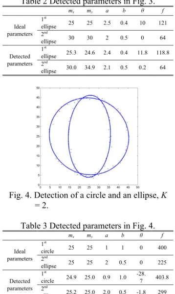
N(0, 0.5) × N(0, 0.5). Fig. 4. Detection of a circle and an ellipse, K

= 2. In initial stage, mx and my are randomly

distributed over (0, 50), fk = 0, ak = 1, bk = 1,

and θk = 0. The cooling function is T(t) =

Tmax × 0.98(t-1), for t = 1, 2, 3, …, with a high

enough temperature, Tmax = 500. We have

100 trials in one temperature. The temperature decreases 500 times to T = 0.0209, and this temperature is low enough. Set constants, αm = 1, αab = 1, αθ = 2, and αf

= 2.

Table 3 Detected parameters in Fig. 4.

mx my a b θ f Ideal parameters 1st circle 25 25 1 1 0 400 2nd ellipse 25 25 2 0.5 0 225 Detected parameters 1st circle 24.9 25.0 0.9 1.0 -28. 7 403.8 2nd ellipse 25.2 25.0 2.0 0.5 -1.8 299

Fig. 3-Fig. 6 show the detection results. Table 2-5 list the ideal and detected parameters in each figure. The results are quite successful.

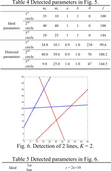
Fig. 5. Detection of three circles, K = 3.

(5)

Table 4 Detected parameters in Fig. 5. mx my a b θ f Ideal parameters 1st circle 35 10 1 1 0 100 2nd circle 40 40 1 1 0 100 3rd circle 10 25 1 1 0 144 Detected parameters 1st circle 34.8 10.1 0.9 1.0 238 99.6 2nd circle 40.0 39.6 0.9 1.0 70 100.2 3rd circle 9.8 25.0 1.0 1.0 47 144.5

Fig. 6. Detection of 2 lines, K = 2. Table 5 Detected parameters in Fig. 6.

Ideal parameter s 1st line y = 2x+10 2nd line x = x-10 mx my a b θ f Detected parameter s 1st line 25.4 15.7 -0.7 1.5 258 0(preset) 2nd line 7.68 25.4 -0.6 1.8 213 0(preset) (2) 討論:

We propose a system that adopts the simulated annealing algorithm to detect patterns such as lines, circles, and ellipses by finding their parameters in an unsupervised manner and global minimum fitting error related to points in an image. Also, we define the distance from a point to all patterns and this makes the computation feasible. Using four steps to adjust parameters through center, shape, angle, and the size of the pattern can get fast convergence. Experimental results on the detection of these patterns in images are successful.

The system can be extended to

hyperbolic pattern detection in the future. Also the determination of the number of patterns, parameters setting, and the initial temperature are the future work.

四、成果自評研究內容與原計畫相符程度: 100% 達成預期目標情況: 100% 研究成果的學術或應用價值: 利用模擬退火的全域最佳化特性求取影像中圖形 (直線、圓、橢圓)的參數，對於影像處理有實質的貢獻。是否適合在學術期刊發表: 是主要發現或其他有關價值: 可將系統做延伸用於震測信號的處理與解釋上。 五、參考文獻

[1] Hough, P.V.C., Method and means for recognizing complex patterns: U.S. Patent 3069654, 1962.

[2] Duda, R.O., and Hart, P.E., Use of the Hough transform to detect lines and curves in pictures: Communications of the ACM, 15, 11-15, 1972

[3] Basak, J. and Das, A., Hough transform networks: Learning conoidal structures in a connectionist framework: IEEE Transactions on Neural Networks, 13, no. 2, 381-392, 2002.

[4] Basak, J. and Das, A., Hough transform network: A Class of networks for identifying parametric structures: Neurocomputing, 51, 125-145, 2003.

[5] S. Kirkpatrick, C. D. Gelatt, and M. P. Vecchi, “Optimization by simulated annealing,” Science, vol. 220, pp. 671-680, 1983.

[6] A. Corana, M. Marchesi, C. Martini, and S. Ridella, “Minimizing multimodal functions of continuous variables with the simulated annealing algorithm,” ACM Transactions on Mathematical Software, vol. 13, pp. 262-280, 1987.