應用影像融合技術於彩色影像之對比強化演算法

(1)

國

立

交

通

大

學

多媒體工程研究所

碩

士

論

文

應用影像融合技術於彩色影像之對比強化演算法

Color Image Contrast Enhancement Using Image Fusion Technique

研究生：王維綱

指導教授：陳玲慧教授

指導教授：李建興教授

(2)

應用影像融合技術於彩色影像之對比強化演算法

Color Image Contrast Enhancement Using Image Fusion Technique

研究生：王維綱 Student：Wei-Kang Wang

指導教授：陳玲慧 Advisor：Ling-Hwei Chen

指導教授：李建興 Advisor：Chang-Hsing Lee

國立交通大學

多媒體工程研究所

碩士論文

A Thesis

Submitted to Institute of Multimedia Engineering College of Computer Science

National Chiao Tung University in partial Fulfillment of the Requirements

for the Degree of Master

in

Computer Science

July 2012

Hsinchu, Taiwan, Republic of China

(3)

i

應用影像融合技術於彩色影像之

對比強化演算法

研究生：王維綱指導教授：陳玲慧博士

李建興博士

國立交通大學多媒體工程研究所碩士班

摘要

由於攝影器材（例如數位相機和手機）的發展與普及，越來越多的數位影像出現在人們的日常生活中。同時，隨著網際網路與社群網路逐漸發展成熟，人們可以很輕易的與朋友分享彼此的影像。但是並不是所有的影像都是讓人滿意的。攝影器材的技術限制以及不適當的攝影環境會使得有些影像曝光不夠而有些影像則是過度曝光。為了能夠解決這個問題，許多傳統的影像強化技術被提出來。但是這些傳統技術經常只適用於一些特定的影像抑或這些方法是非自動化的。因此，本論文提供了一個基於影像融合技術的對比強化演算法。首先，數張亮度不同的影像會被產生出來。接著，輸入影像的像素會依據像素的亮度來做分群。最後，我們提出的 Classified Image Fusion (CIF)方法會將這些虛擬影像作結合來得到一張曝光良好的結合後的影像。

(4)

ii

Color Image Contrast Enhancement Using

Image Fusion Technique

Student：Wei-Kang Wang Advisor：Dr. Ling-Hwei Chen

Dr. Chang-Hsing Lee

Institute of Multimedia Engineering

College of Computer Science

National Chiao Tung University

ABSTRACT

There are more and more digital images in our daily life thanks to the popularity

of photograph capturing equipments, such as digital cameras and mobile phones. In

addition, as the Internet and social networks have been well developed, it’s easier for

people to share images with their friends. However, not all people are satisfied with

the photos they taken due to the limitations of the image capturing devices. The

improper luminance condition may cause under-exposed and over-exposed images.

To solve this problem, plenty of researches are proposed for contrast enhancement.

(5)

iii

low contrast images or cannot be automatically applied on all images. Hence, in this

thesis, we propose a classified image fusion (CIF) method for image contrast

enhancement. First several virtual images having different intensities are generated.

Second, the input image pixels are classified to several classes according to their

luminance values. Finally, CIF was proposed to combine these exposure images to

(6)

iv

誌謝

這篇論文的完成，首先感謝指導教授陳玲惠博士和李建興博士。謝謝兩位教授兩年間不辭辛勞的給予課業上及生活上的指導與關心。讓我在攻讀交通大學碩士的這兩年間，除了學習到如何做研究外，也學會了很多待人處事的道理。此外，也感謝口試委員李坤龍教授、石昭玲教授和李遠坤教授於口試中給予的建議與指導，使我能夠發現自己研究的盲點與潛力，也使的整篇論文更佳的完善。在碩士的兩年間，最常出現也待最久的地方就是實驗室了。非常感謝實驗室文超、惠龍、俊旻、占和、芳如、盈如和懷三學長們對我的指導與建議。謝謝他們教導了我不只是課業上的知識也教了我很多生活上的態度。感謝昱嘉、志錡、明昌三位學弟，有了他們讓實驗是充滿了朝氣與歡笑。感謝厚邑和子杰兩個我從大學時代起的好朋友，我們一起努力完成了碩士的學業、通過了最後口試的考驗。謝謝你們照兩年的陪伴與對我的照顧，萬分感謝。此外，這裡還想要謝謝我的朋友們，感謝他們對我的鼓勵與關心。感謝我的國中死黨們，即使沒有直接的話語，但是我知道你們一直都是支持我、關心我的。最後我想要感謝我的家人，感謝我的爸爸、媽媽、哥哥和弟弟，謝謝爸媽一直對我的鼓勵與支持，謝謝哥哥給我碩士生過來人的一些經驗，謝謝弟弟陪我一起宣洩我的壓力，有你們、有這個溫暖的家，讓我迷茫、疲憊、挫折時，能夠堅強的再站起來並鼓起勇氣去面對每一個挑戰。謹以此篇論文獻給你們，也獻給所有我關心以及關心我的人。

(7)

v

LIST OF FIGURES

Fig. 1 Flow chart of the proposed CIF system ………..……10 Fig. 2 Generated virtual exposure images (a) k = -7 (b) k = -6 (c) k = -5 (d) k = -4 (e)

k = -3 (f) k = -2 (g) k = -1 (h) k = 0 (original image) (i) k = 1 (j) k = 2 (k) k =

3 (l) k = 4 (m) k = 5 (n) k = 6 (o) k = 7………...12

Fig. 3 Generated virtual exposure images (a) k = -7 (b) k = -6 (c) k = -5 (d) k = -4

(e) k = -3 (f) k = -2 (g) k = -1 (h) k = 0 (original image) (i) k = 1 (j) k = 2 (k) k = 3 (l) k = 4 (m) k = 5 (n) k = 6 (o) k = 7 ………...…13

Fig. 4 Input images and classification results. (a) Original gray image (b)

Classification result with m = 3 (c) Original gray image (d) Classification result with m = 4 (e) Original gray image (f) Classification result with……16

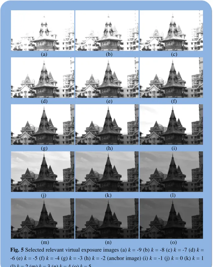
Fig. 5 Selected relevant virtual exposure images (a) k = -9 (b) k = -8 (c) k = -7 (d) k

= -6 (e) k = -5 (f) k = -4 (g) k = -3 (h) k = -2 (anchor image) (i) k = -1 (j) k = 0 (k) k = 1 (l) k = 2 (m) k = 3 (n) k = 4 (o) k = 5 ………...18

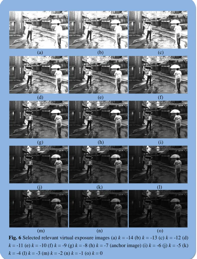
Fig. 6 Selected relevant virtual exposure images (a) k = -14 (b) k = -13 (c) k = -12

(d) k = -11 (e) k = -10 (f) k = -9 (g) k = -8 (h) k = -7 (anchor image) (i) k = -6 (j) k = -5 (k) k = -4 (l) k = -3 (m) k = -2 (n) k = -1 (o) k = 0………….……..19

Fig. 7 Flow chart of the proposed classified image fusion method ……….20 Fig. 8 The mask B used in computing bg(x, y) ………..………..22 Fig. 9 The gradient mask used in computing gradk(x, y) …………...22

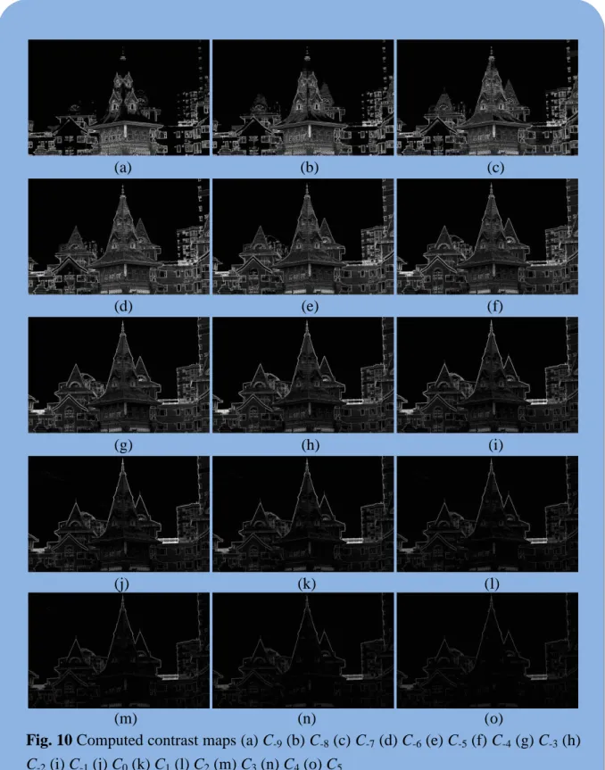
Fig. 10 Computed contrast maps (a) C-9 (b) C-8 (c) C-7 (d) C-6 (e) C-5 (f) C-4 (g) C-3 (h)

C-2 (i) C-1 (j) C0 (k) C1 (l) C2 (m) C3 (n) C4 (o) C5………...…..24

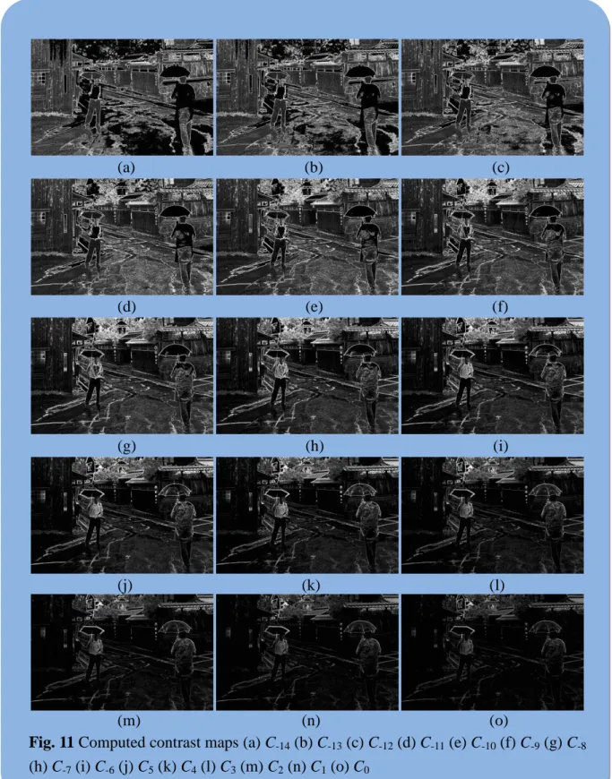
Fig. 11 Computed contrast maps (a) C-14 (b) C-13 (c) C-12 (d) C-11 (e) C-10 (f) C-9 (g)

C-8 (h) C-7 (i) C-6 (j) C5 (k) C4 (l) C3 (m) C2 (n) C1 (o) C0 ………25

Fig. 12 The equally-distributed target luminance values t i

Y with m = 3 ..………..27

Fig. 13 The target luminance values P i

Y with m = 3 ………..…28

Fig. 14 The luminance range to determine σi with m = 3 .……….30

Fig. 15 Exposedness maps generated by using the exposedness measure proposed by

Mertens et al. [22] (a) E-9 (b) E-8 (c) E-7 (d) E-6 (e) E-5 (f) E-4 (g) E-3 (h) E-2 (i)

E-1 (j) E0 (k) E1 (l) E2 (m) E3 (n) E4 (o) E5 ………....32

Fig. 16 Classified well-exposedness maps (a) E-9 (b) E-8 (c) E-7 (d) E-6 (e) E-5 (f) E-4

(g) E-3 (h) E-2 (i) E-1 (j) E0 (k) E1 (l) E2 (m) E3 (n) E4 (o) E5 ….……...33

Mertens et al. [22] (a) E-14 (b) E-13 (c) E-12 (d) E-11 (e) E-10 (f) E-9 (g) E-8 (h)

(10)

viii

Fig. 18 Classified well-exposedness maps (a) E-14 (b) E-13 (c) E-12 (d) E-11 (e) E-10 (f)

E-9 (g) E-8 (h) E-7 (i) E-6 (j) E-5 (k) E-4 (l) E-3 (m) E-2 (n) E-1 (o) E0 …….35

Fig. 19 Weight maps, Wk, of each exposure image Yk generated by using the

proposed classified exposedness measure. (a) W-9 (b) W-8 (c) W-7 (d) W-6 (e)

W-5 (f) W-4 (g) W-3 (h) W-2 (i) W-1 (j) W0 (k) W1 (l) W2 (m) W3 (n) W4 (o)

W5 ………37

Fig. 20 Weight maps, Wk, of each exposure image Yk generated by using the

proposed classified exposedness measure. (a) W-14 (b) W-13 (c) W-12 (d) W-11

(e) W-10 (f) W-9 (g) W-8 (h) W-7 (i) W-6 (j) W-5 (k) W-4 (l) W-3 (m) W-2 (n) W-1

(o) W0 ………38

Fig. 21 Enhanced results of a normal image using different methods ……….…...47 Fig. 22 Enhanced results of a backlight image using different methods ……..…….48 Fig. 23 Enhanced results of a low contrast image using different methods …..……49 Fig. 24 Enhanced results of another low contrast image using different methods …50 Fig. 25 Enhanced results of a dark scene image using different methods ………….51 Fig. 26 Enhanced results of a dark scene image using different methods ………….52 Fig. 27 Enhanced results of a dark scene image using different methods ………….53

(11)

1

CHAPTER 1 INTRODUCTION

1.1 Motivation

There are more and more digital images in our daily life thanks to the popularity

of photograph capturing equipments, such as digital cameras and mobile phones. In

addition, as the Internet and social networks have been widely developed, it’s easier

for people to share images with their friends. However, not all people are satisfied

with the photos they taken due to the limitations of image capturing devices. Typically,

the dynamic ranges of digital cameras or mobile phones are much smaller than that

human eyes can perceive. This phenomenon becomes more apparent in high dynamic

regions such as skies or shadows. The common shortages found in real-life images

include:

(1) A normal image with suitable exposure but some under-exposed and/or

some over-exposed regions;

(2) An over-exposed image;

(12)

2

1.2 Related Work

In order to obtain an image with proper exposedness and contrast, an image

contrast enhancement technique is needed. There are plenty of researches proposed

for image contrast enhancement. These methods can be classified into four major

categories:

(1) Histogram-based methods [1-7];

(2) Transform-based methods [1], [8], [9];

(3) Exposure-based methods [10], [11];

(4) Image fusion based methods [12-14].

The most common and well-known histogram-based method is histogram

equalization (HE) [1]. HE adjusts the input image histogram by using a non-linear

mapping function to yield a histogram which approximates uniform distribution. It

will spread the gray levels with high occurring probabilities and compress the gray

levels with low occurring probabilities to obtain an image having better contrast.

However, HE was proved to produce some unwanted artifacts, including

(1) False contour;

(2) Amplified noise;

(3) Washed-out appearance.

(13)

3

[2] proposed a local HE method. First, the input image is divided into several

non-overlapping blocks. Then, HE is applied on each block. The HE enhanced blocks

are finally fused by using bilinear interpolation to reduce the blocking effect. Kim [3]

proposed a subimage independent HE method named brightness preserving

bi-histogram equalization (BBHE). In BBHE, the input gray image is first

decomposed into two subimages based on its mean luminance, μ. Then, HE is applied

to the histograms corresponding to these two subimages independently. The subimage

with luminance lower than the mean value is mapped into the range [lmin, μ], where

lmin denotes the minimum gray level. The subimage with luminance larger than the

mean value is mapped into the range [μ, lmax], where lmax denotes the maximum gray

level. Then, the composition of these two equalized subimages is the output image.

Wang et al. [4] proposed another bi-histogram HE method in which the input image is

decomposed into two subimages by using the threshold value which yields maximum

entropy of the processed image. Then, HE is applied to two subimages independently

and the composition of HE enhanced subimages will form the output image. Chen et

al. [5] extended the former two methods and proposed minimum mean brightness

error bi-histogram equalization (MMBEBHE). In MMBEBHE, the threshold with

minimum absolute mean brightness error (AMBE) is found to divide the input image

(14)

4

composition of the HE result is the output image. Wang et al. [6] used histogram

specification to yield the target histogram which maximizes the entropy under the

constraint that the mean brightness is fixed. Chen et al. [7] proposed a method based

on BBHE. They recursively divide each subimage into two new subimages and finally

perform HE on each portions independently.

Transform-based methods [1], [8], [9] were widely used in electrical devices and

computer software. These methods use a function to map original image luminance

values to another ones. To get a pleasing image, some user-specified parameters are

needed. That is, these methods require some user interactions and thus are not fully

automatic. Transform-based methods can well handle either under-exposed images or

over-exposed images if appropriate parameters are selected. However, they cannot

produce pleasing images when the input images have both under-exposed regions and

over-exposed regions. Moroney [8] proposed a local color correction operation which

uses non-linear masking and a pixel-by-pixel gamma correction to enhance the image

quality. Schettini et al. [9] presented a local and image-dependent exponential

correction method which uses bilateral filter instead of Gaussian filter to avoid halo

effects. However, the global contrast is reduced as well.

Exposure-based methods [10], [11] adjust the exposedness of images by using a

(15)

5

proposed a method which first identifies the information carrying regions and then

adjusts the exposure levels using a “camera response”-like function. In their algorithm,

contrast and focus are used as the measures to identify the information carrying

regions. In addition, skin pixel identification method is applied to find the skin

regions. Then, the mean gray values of those pixels in informative regions are used as

reference values to adjust the exposure levels. Since the technique is designed

specifically to regions of interest, it can produce proper results in those interested

regions. However, other regions may yield poorer illumination. Safonov et al. [11]

provided an exposure correction approach based on contrast stretching and

alpha-blending which considers both brightness and the estimated reflectance of the

input image. The main problem of this method is that it may exhibit unsatisfied

illumination in some regions.

Image fusion based methods [12-14], [22], [26] tried to extract and merge

relevant information from several images taken in the same scene in order to form a

fused image which contains more information and has better visual quality/contrast

than each input image. Hsieh et al. [12] used a linear function to fuse the input image

and a HE enhanced image to produce a fused image. Pei et al. [13] performed HE and

sharpening to the input image and fused together these two enhanced images in the

(16)

6

well-exposedness as image quality measures to evaluate the contribution of each pixel

to the fused image. First, for each input image, a corresponding weight map is

computed. Then, the Laplacian pyramid of the input image and Gaussian pyramid of

the weight map are built respectively. The Laplacian pyramids of the input images are

blended with the corresponding Gaussian pyramid as the weights. Finally, the output

image is produced from the blended Laplacian pyramid. Malik et al. [26] proposed an

image fusion method performed in the wavelet transform domain. The output image is

produced by taken the inverse wavelet transform.

The aforementioned contrast enhancement methods [1-14], [22], [26] often

cannot produce pleasing images for a broad variety of low contrast images or cannot

be automatically applied on all images. That is, some user-specified parameters are

needed to obtain satisfied pictures. Therefore, we tried to design an image contrast

enhancement algorithm which can automatically enhance the contrast without taking

any user-specified parameters for any low contrast images.

In this thesis, we will propose a classified image fusion method for image

contrast enhancement. First, several virtual images having different intensities are

generated. In addition, the input image pixels are classified to several classes

according to their luminance values. Finally, a classified image fusion method,

(17)

7

virtual images and produce a fused image which is well-exposed in every region.

1.3 Organization of the Thesis

The thesis is organized as follows. In Chapter 1, motivation and some related

work are given. In Chapter 2, the proposed classified image fusion method, which can

combine the generated virtual images in an attempt to obtain an image which is

well-exposed in every region. In Chapter 3, experimental results will be given to show

the effectiveness of the proposed method. Finally, a brief conclusion and future work

(18)

8

CHAPTER 2 PROPOSED CLASIFIED IMAGE FUSION METHOD

FOR IMAGE CONTRAST ENHANCEMENT

In this chapter, we will describe the proposed classified image fusion (CIF)

method for image contrast enhancement. Image fusion is the process that aims to

extract relevant information from multiple images taken in the same scene and obtain

a more informative picture with better contrast and image quality. Image fusion has

numerous applications such as remote sensing [15-17], medical imaging [17], high

dynamic range imaging (HDRI) [17], [18], multi-focus imaging [17], [19], etc. In

remote sensing and medical imaging, several images captured from various sensors

are given. Then, these images are fused to produce a high quality image. In HDRI,

multiple images taken in the same scene with different exposure time are generated.

The image pixels having distinct luminance values are then fused to yield an image

having wide dynamic range than each individual one. In multi-focus imaging, several

images with each having some objects in focus will be merged to obtain an image in

which all relevant objects are in focus. For these applications, several images with

varying luminance, exposure, or focus, should be obtained in advance. However, it is

(19)

9

the same scene with variant information. Therefore, an algorithm will be proposed to

produce several virtual images for image fusion.

Since our proposed CIF method works on gray images, a color value to gray

value conversion is first applied on each input color image. The luminance image Y(x,

y) is converted from its original red, blue, green components using the following

function: ). , ( 114 . 0 ) , ( 587 . 0 ) , ( 299 . 0 ) , (x y R x y G x y B x y Y       (1)

where R(x, y), G(x, y), and B(x, y) denote red, green and blue color values of the pixel

located at (x, y). Then, several virtual images having different intensities are generated.

In addition, a multilevel thresholding algorithm is employed to classify the input

image pixels to different classes depending on their luminance values. By using the

classification result, several relevant virtual images are selected among the generated

virtual images. After the relevant virtual images are selected, the proposed classified

image fusion algorithm, performed in discrete wavelet transform (DWT) domain, will

be designed to obtain a fused image with proper exposure in every region. The flow

(20)

10

2.1 Generation of Virtual Exposure Images

In image fusion, several images are combined to produce an output image having

better quality. For image enhancement, only one input image is given to produce an

output image with higher contrast. Therefore, it is necessary to design an algorithm to

generate several virtual images such that image fusion technique can be applied for

image contrast enhancement. In the proposed CIF method, the concept of exposure,

which refers to how much light will reach the image sensors on image capturing

devices, will be exploited to generate several virtual images having distinct luminance.

For digital cameras, shutter speed and F-stop are used to determine the exposure when

taking photos. Shutter speed controls how long the shutter is open, which corresponds

to the length of time the light can reach the image sensors. The larger the shutter

speed, the more the amount of light reaching the image sensors. Another factor

controlling the exposure of a photo is F-stop, which controls the size of the aperture.

The aperture is the hole the light of the scene passing through in the digital cameras.

(21)

11

Modern cameras use a standard F-stop scale: f/1, f/1.4, f/2, f/2.8, f/4, f/5.6, f/8, f/11,

f/16, f/22, etc. The scale is an approximately geometric sequence that corresponds to

the sequence of the powers of the square of 2. In this sequence, each stop represents a

halving of the light intensity from the previous stop. For example, f/1 allows twice as

much light to fall on the image sensor than f/1.4, and four times as much light than f/2.

In this study, we exploit the F-stop concept to generate virtual images such that their

pixel luminance values approximate a geometric sequence. In this thesis, the

luminance of the k-th virtual exposure image, denoted by Yk, is defined by the

following equation:           otherwise , 255 255 2 ) ( if , 2 ) , ( ) , ( 4 4 k k x,y Y y x Y y x Yk (2)

where Y(x, y) is the gray level of input image pixel located at (x, y).

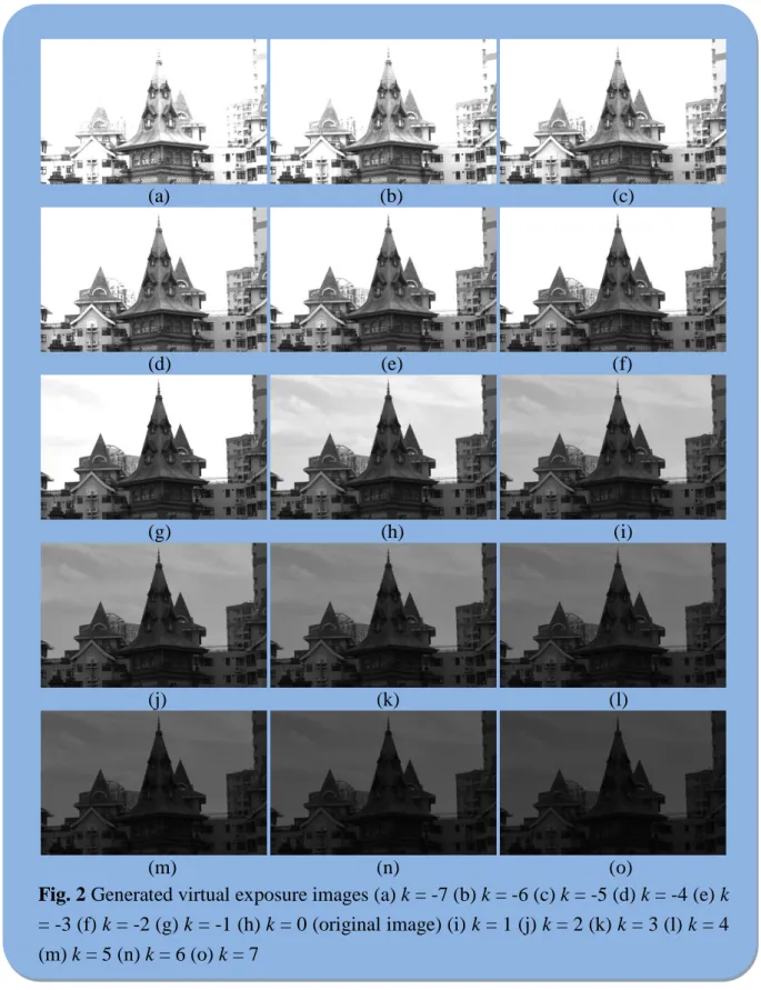
From Eq. (2), N brighter images (with k N,-N1,...,1) and N darker images (with k 1,2,...,N) compared to the input image Y are generated. Fig. 2 and Fig. 3 show some generated virtual exposure images. From Fig. 2, we can see that in

those brighter virtual images, the detail of the central building becomes more apparent

and the contrast is much sharper than that in the original image (with k = 0). However,

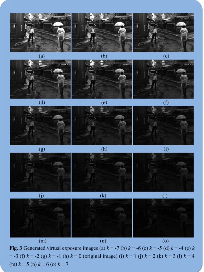
the contrast in the sky region becomes less sharp in these brighter images. Fig. 3

shows a similar result. That is, the detail of the dark foreground objects becomes

(22)

12 (a) (b) (c) (d) (e) (f) (g) (h) (i) (j) (k) (l) (m) (n) (o)

Fig. 2 Generated virtual exposure images (a) k = -7 (b) k = -6 (c) k = -5 (d) k = -4 (e) k

= -3 (f) k = -2 (g) k = -1 (h) k = 0 (original image) (i) k = 1 (j) k = 2 (k) k = 3 (l) k = 4 (m) k = 5 (n) k = 6 (o) k = 7

(23)

Fig. 3 Generated virtual exposure images (a) k = -7 (b) k = -6 (c) k = -5 (d) k = -4 (e) k

= -3 (f) k = -2 (g) k = -1 (h) k = 0 (original image) (i) k = 1 (j) k = 2 (k) k = 3 (l) k = 4 (m) k = 5 (n) k = 6 (o) k = 7

(24)

14

2.2 Image Pixel Classification

In the proposed CIF method, the input image pixels are classified to m classes.

Pixels in different classes will be blended with different image fusion rules. A

multilevel thresholding algorithm designed by Liao et al. [20] is utilized to find m-1

thresholds, denoted by Thd1, Thd2, …, Thdm-1 (Thd1 < Thd2 < … < Thdm-1), to divide

the input image pixels into m classes. Let Ω1, Ω2, …, Ωm denote these m classes,

according to the m-1 thresholds, these classes can be defined as follows:



( , )| ( , ) ₁



. 1 x y Y x y Thd  (3)



(x,y)|Thd_i₁ Y(x,y) Thd_i



for i 2,...,m-1. i     _ (4)



( , )| ( , ) _₁



.  _m x y Y x y Thd_m (5)

In order to determine the proper cluster number m, a metric called Dunn index (DI)

[20] will be used to evaluate the classification results. DI was defined to get a

clustering result having small within-class variance and a large between-class

variance. The definition of DI for n classes is given by:

k j i c c DI k n k j i i j n j i n , , , max ) , ( min 1 , , 1 _         (6)

where (c_i,c_j) denotes the distance between two cluster centers of Ωi and Ωj

(between-class variance) and Δk is defined as follows:

). , ( max ,q kd p q p k __  (7)

(25)

15

variance). The higher DI indicates the better clustering result. Based on Eq. (6), the

cluster number m is determined by:

. max arg max min n m n m DI m    ₍₈₎

where mmin and mmax are the maximum and minimum cluster number to be examined.

To save computation time, we bound the cluster number in the range from 3 to 6. That

is, set mmin = 3 and mmax = 6. This setting is based on the observation that typically an

image has at least three classes: dark pixels, bright pixels, and pixels with luminance

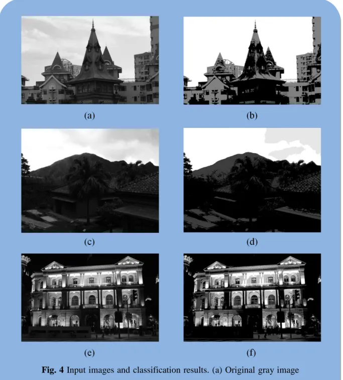
values in-between. Fig. 4 shows three input images and the corresponding image pixel

classification results. The input image shown in Fig. 4(a) is classified to three classes

as shown in Fig. 4(b): the sky region (the bright pixels), the background buildings

(well-exposed pixels), and the front-central building (dark pixels). Fig. 4(c) shows an

input image which is classified to four classes as shown in Fig. 4(d): the left side of

the sky region, the right side of the sky region, the background mountain, and the dark

houses. In Fig. 4(c), since the right side of the sky is visibly darker than the left side

of the sky, they are separated to two classes. Similarly, the right side of the sky is

noticeable brighter than the background mountain and the roof of the houses, they are

also separated. Finally, the dark trees, parts of the houses and the wall are classified to

the dark pixels. Fig. 4(f) shows the classification result of Fig. 4(e) which is classified

(26)

16

Fig. 4 Input images and classification results. (a) Original gray image

(b) Classification result with m = 3 (c) Original gray image (d) Classification result with m = 4 (e) Original gray image (f) Classification result with m = 5

(27)

17

2.3 Selection of Relevant Virtual Exposure Images

The previously generated 2N+1 images are not all used in the image fusion

process. Among these 2N+1 virtual exposure images, only those images having some

relevant informative regions will be chosen for image fusion. That is, those images

which are completely under-exposed or completely over-exposed will not be used in

the image fusion process in an attempt to yield a high informative fused image. To

this end, an anchor image among these 2N+1 virtual exposure images will be selected

first. For virtual image Yk, the trimmed mean luminance, denoted byk,of the image

pixels belonging to clusters Ω2, Ω3, …, Ωm-1 is calculated:

. Ω ) , ( 1 2 Ω ,..., Ω ) , ( ₂ ₁



     _m i i y x k k m y x Y  (9)

That is, the pixels in the darkest class C1 and the brightest class Cm are not considered.

The image having a trimmed mean luminance_kclosest to gray level 128 (the middle

value in the luminance range [0, 255]) will be selected as the anchor image:

. | 128 | min arg ,...,     N N k k anc  (10)

The anchor image and its preceding M (M  N) brighter images and succeeding M

darker images, denoted by Yanc-M, …, Yanc, …, Yanc+M,, will yield the final set of virtual

exposure images for image fusion. Fig. 5 and Fig. 6 show two examples of selected

(28)

18

we can see that those dark virtual images which are less informative are excluded for

image fusion process.

(a) (b) (c)

(d) (e) (f)

(g) (h) (i)

(j) (k) (l)

(m) (n) (o)

Fig. 5 Selected relevant virtual exposure images (a) k = -9 (b) k = -8 (c) k = -7 (d) k =

-6 (e) k = -5 (f) k = -4 (g) k = -3 (h) k = -2 (anchor image) (i) k = -1 (j) k = 0 (k) k = 1 (l) k = 2 (m) k = 3 (n) k = 4 (o) k = 5

(29)

Fig. 6 Selected relevant virtual exposure images (a) k = -14 (b) k = -13 (c) k = -12 (d)

k = -11 (e) k = -10 (f) k = -9 (g) k = -8 (h) k = -7 (anchor image) (i) k = -6 (j) k = -5 (k) k = -4 (l) k = -3 (m) k = -2 (n) k = -1 (o) k = 0

(30)

20

2.4 Classified Image Fusion

The 2M+1 virtual exposure images, denoted by Yk (k = anc-M, …, anc, …,

anc+M), having different intensities are then blended by using the proposed classified

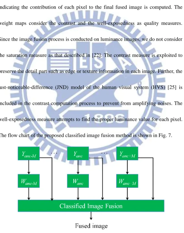
image fusion method. First, for every virtual exposure image Yk, a weighted map Wk

indicating the contribution of each pixel to the final fused image is computed. The

weight maps consider the contrast and the well-exposedness as quality measures.

Since the image fusion process is conducted on luminance images, we do not consider

the saturation measure as that described in [22]. The contrast measure is exploited to

preserve the detail part such as edge or texture information in each image. Further, the

just-noticeable-difference (JND) model of the human visual system (HVS) [25] is

included in the contrast computation process to prevent from amplifying noises. The

well-exposedness measure attempts to find the proper luminance value for each pixel.

The flow chart of the proposed classified image fusion method is shown in Fig. 7.

(31)

21

2.4.1 Just-Noticeable-Difference (JND) Model of the Human Visual

System (HVS)

JND determines the threshold of luminance difference that can be perceived by

HVS. In this thesis, the JND model proposed by Chou and Li [25], determined by the

average background intensity and the spatial non-uniformity, will be used for quality

measure evaluation. The JND value of the image pixel located at (x, y) is defined as

follows:



( ( , ), ( , )), ( ( , ))



. max ) , (x y J₁ bg x y mg x y J₂ bg x y JND  (11)

where J1 models the spatial masking effect and is defined by:

)). , ( ( )) , ( ( ) , ( )) , ( ), , ( ( 1 bg x y mg x y mg x y bg x y bg x y J 







(12)

where α(x) and β(x) are defined as follows:

, 115 . 0 0001 . 0 ) (x x   (13) , 01 . 0 ) (x x  (14)

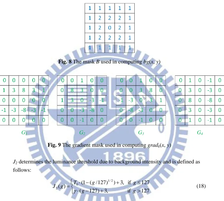
where λ influences the visibility threshold due to spatial masking effect, bg(x, y) is the

average background intensity computed by using the mask B (as shown in Fig. 8):

. ) 2 , 2 ( ) , ( 32 1 ) , ( 2 2 2 2

 

        i j j i B j y i x Y y x bg (15)

mg(x, y) is the maximum gradient value in four directions:

|}. ) , ( {| max ) , ( 4 , 3 , 2 , 1 grad x y y x mg k k  (16)

(32)

22 . ) 2 , 2 ( ) , ( 16 1 ) , ( 2 2 2 2

 

        i j k k x y Y x i y j G i j grad (17)

where Gk is the k-th gradient mask as shown in Fig. 9.

Fig. 8 The mask B used in computing bg(x, y)

G1 G2 G3 G4

Fig. 9 The gradient mask used in computing gradk(x, y)

J2 determines the luminance threshold due to background intensity and is defined as

follows:             127 if , 3 ) 127 ( 127 if , 3 ) ) 127 / ( 1 ( ) ( 2 / 1 0 2 g g g g T g J  (18)

where T0 and γ depend on the viewing distance between the monitor and the tester,T0

denotes the visibility threshold when the background gray level is 0, and γ denotes the

slope of the line that models the JND visibility threshold function at higher

background luminance. In this thesis, we set T0 = 17, γ = 3/128, and λ = 1/2 as

(33)

23

2.4.2 Contrast Measure

To measure the contrast of a pixel p located at (x, y) in the virtual image Yk, we

find the maximum and the minimum values (denoted by Y_kmax(x,y) and Y_kmin(x,y)) of its eight neighbors within a 3×3 window centered at p. Then the difference

) , (x y

Y_kdif between Y_kmax(x,y) and Y_kmin(x,y) is calculated: ). , ( ) , ( ) , (x y Ymax x y Ymin x y Y_kdif  _k  _k (19)

The difference can be considered as a simple contrast value for pixel p. If the

difference is smaller than its corresponding JND value JND_k(x,y), which implies

that there is no visible edge or texture information, the contrast measure is set to 0.

Otherwise, we set the contrast value as Y_kdif(x,y). To prevent from zero weight value and variant range for different quality measures, the contrast measure for pixel p is

normalized by using the following equation:

       otherwise , 256 / ) 1 ) , ( ( ) ( ) ( if , 256 / 1 ) , ( y x Y x,y JND x,y Y y x C dif k k dif k k (20)

where C_k(x,y) denotes the contrast value for the pixel located at (x, y) in exposure

image Yk. For each virtual exposure image Yk, a corresponding contrast map Ck is

computed. In total, 2M+1 contrast maps are computed. Fig. 10 and Fig. 11 show the

(34)

Fig. 10 Computed contrast maps (a) C-9 (b) C-8 (c) C-7 (d) C-6 (e) C-5 (f) C-4 (g) C-3 (h)

(35)

Fig. 11 Computed contrast maps (a) C-14 (b) C-13 (c) C-12 (d) C-11 (e) C-10 (f) C-9 (g) C-8

(36)

26

2.4.3 Well-exposedness Measure

Well-exposedness measure evaluates how well a pixel is exposed. Mertens et al.

[22] utilized a Gaussian distribution to model the exposedness of a pixel depending on

how close its luminance is to the target luminance values 128 (the middle value of

luminance range [0, 255]). That is, the pixels with luminance value closer to gray

level 128 should have a larger weight while the pixels with luminance far away from

128 should have a smaller weight when computing the well-exposedness measure.

Generally, the well-exposedness measure is defined as follows [22]:

. 2 ) 128 ) , ( ( exp ) , ( ₂ 2      _    y x Y y x E k k (21)

where Ek(x, y) is the well-exposedness value of the pixel located at (x, y), and σ is the

standard deviation of the Gaussian distribution which is set as 0.2×255 (the luminance

range). From Eq. (21), the well-exposedness value is bounded to be the range [0, 1].

Further, the pixel with luminance value closer to gray level 128 will be assigned a

larger exposedness value. Consequently, the luminance of each pixel in the fused

image will be adjusted toward 128. However, this does not make sense for real-life

images. For example, all dark pixels and bright pixels will be both adjusted toward

128. As a result, the global contrast will be reduced. To solve this problem, we

classify the pixels in the original image into different classes according to their

(37)

27

different classes. Intuitively, the target luminance values Y_it (i = 1, 2, …, m) can be determined by finding the center of each equally-spaced interval (see Fig. 12 for an

example with cluster number m = 3).

Fig. 12 The equally-distributed target luminance values Y_it with m = 3.

This method assumes that the whole luminance range (256) is divided into m

equally-spaced intervals having width R = 256/m. Further assuming that the

luminance values in each class are Gaussian distributed with width equals R = 6σe

where σe is the standard deviation of the Gaussian distribution. Thus, the target

luminance value associated with class Ωi is

. ) 2 1 (i R Y_it    (22)

However, the equally-spaced target luminance values, without considering property of

the input image, should be adjusted to appropriate values. For example, if the input

image is a dark one consisting of many dark pixels in Ω1, the target luminance value

t

Y₁ should be adjusted as well. Similarly, if the input image is a bright one consisting

of many bright pixels in Ωm, the target luminance value Ymt should be adjusted in

(38)

28

the number of pixels in each class, will take into account the image property to find

target luminance values. Let pi denote the probability of the pixels belonging to class

Ωi in the input image. Then, the cumulative probability Cum(i) for each class Ωi is

defined as follows:



  i k k p i Cum 1 ) ( (23)

Thus, the target luminance range associated with class Ωi is [Cum(i-1)×255,

Cum(i)×255] (see Fig. 13) for 1im, where Cum(i) is defined as 0.

Fig. 13 The target luminance values Y_iPwith m = 3.

According to the probability of each class, the target luminance value is defined as the

middle value in each target luminance range:

m ..., , , i i Cum i Cum Y_iP ), for 12 2 ) ( ) 1 ( ( 255     (24)

Further, the mean luminance value of the pixels belonging to the largest class is

used to determine whether an input image is a dark one or a bright one. Let Ni denote

the number of pixels belonging to class Ωi. The index of the largest class is defined as

follows: . max arg 1 max i m i N n    (25)

Then the mean luminance value of the largest class _no

max

(39)

29 , ) , ( m a x m a x m a x ) , ( n y x o n n y x Y  



  (26)

Finally, Y_it is defined as follows:









i , ,...,m Y R i Y R i Y P i P i t i for 1 2 128 if , , ) 2 / 1 ( min 128 if , , ) 2 / 1 ( max o n o n max max               (27)

If the pixel belongs to Ωi, the pixel luminance value will be adjusted toward Yit.

However, if the luminance value of a pixel is near the boundary of two classes, it is

hard to determine which class this pixel really belongs to. That is, it is hard to

determine its target luminance value and thus it is impossible to correctly evaluate the

appropriate exposedness value. Therefore, we exploit the concept of fuzzy clustering

to determine the probability that a pixel belongs to a class. Let _io denote in the input image the average luminance of those pixels belonging to cluster Ωi:

m i y x Y i y x o i i ..., , 2 , 1 for , ) , ( ) , (   



  (28)

Then, the probability, computed as the likelihood that a pixel value is from each class,

is modeled as a Gaussian function:

, 2 ) ) , ( ( exp ) , ( ₂ 2      _   i o i i y x Y y x P   (29)

where Y is the input image, σi is the standard deviation computed from the luminance

values of those pixels having luminance values in the range [_{i 1}o, i 1o ]. Note that o

0

 is set to 0 and _{m 1}o is set to 255. Since the range [ 1,

o i

 o i 1

(40)

30

with 1im and thus the corresponding standard deviation is multiplied by 0.75 such that every σi is computed from similar range. Fig. 14 illustrates the above

concept.

Fig. 14 The luminance range for determining σi with m = 3.

To utilize the fuzzy clustering concept, the well-exposedness value of the pixel in Yk

associated with class Ωi is defined as follows:

m ..., , , i Y y x Y y x W e t i k e i k ,for 12 ) 2 ( 2 ) ) , ( ( exp ) , ( ₂ 2 ,       _    (30)

Finally, the well-exposedness is defined by:

). , ( ) , ( ) , ( _, 1 P x y W x y Max y x E e i k i m i k  __  (31)

where Ek(x, y) denotes the well-exposedness value associated with the pixel located at

(x, y) in virtual exposure image Yk. By applying different target luminance values to

different classes, pixels will be adjusted toward different luminance value and thus the

global contrast can be reserved. Fig. 15 and Fig. 16 show the well-exposedness maps

produced by using the exposedness measure computed by using a single target

(41)

31

exposedness measure. From Fig. 15, by observing the sky region, we can see that

those lower exposure dark images have larger weight values than those in the brighter

images. As a result, the luminance of the sky region will decrease in the fused image.

From Fig. 16, however, by using the proposed method, E-2 has larger weight values in

the sky region and can preserve the luminance much better than Mertens’s method.

Fig. 17 and Fig. 18 show another example of computed well-exposedness maps by

using the exposedness measure proposed by Mertens el al. [22] and the proposed

(42)

Mertens et al. [22] (a) E-9 (b) E-8 (c) E-7 (d) E-6 (e) E-5 (f) E-4 (g) E-3 (h) E-2 (i) E-1 (j)

(43)

Fig. 16 Classified well-exposedness maps (a) E-9 (b) E-8 (c) E-7 (d) E-6 (e) E-5 (f) E-4 (g)

(44)

Mertens et al. [22] (a) E-14 (b) E-13 (c) E-12 (d) E-11 (e) E-10 (f) E-9 (g) E-8 (h) E-7 (i) E-6

(45)

Fig. 18 Classified well-exposedness maps (a) E-14 (b) E-13 (c) E-12 (d) E-11 (e) E-10 (f)

(46)

36

Finally, W_kt, denoting the weight map of the virtual exposure image Yk, is

defined as the multiplication of Ck_{and E}k:

). , ( ) , ( ) , (x y C x y E x y W_kt  _k  _k (32)

Because the fused image is the weighted average of these 2M+1 virtual exposure

images, we normalize each weight map, W_kt, such that for each pixel (x, y), the sum of weights among these 2M+1 weight maps equals 1:

. ) , ( ) , ( ) , (



    _anc_M M anc i t i t k k y x W y x W y x W (33)

Fig. 19 and Fig. 20 show two example of final weight maps produced by multiplying

(47)

Fig 19 Weight maps, Wk,of each exposure image Yk generated by using the proposed

classified exposedness measure. (a) W-9 (b) W-8 (c) W-7 (d) W-6 (e) W-5 (f) W-4 (g) W-3

(48)

Fig 20 Weight maps, Wk,of each exposure image Yk generated by using the proposed

classified exposedness measure. (a) W-14 (b) W-13 (c) W-12 (d) W-11 (e) W-10 (f) W-9 (g)

(49)

39

2.4.4 Classified Image Fusion in the DWT Domain

Mertens et al. [22] have shown that if images are directly fused in the spatial

domain, there will be annoying seams at pixels where weight values change quickly.

To solve this problem, they blend the images in multiple resolutions realized by using

image pyramid decomposition. First, a Laplacian pyramid is built for each exposure

image and a Gaussian pyramid is constructed for each weight map. Then the

coefficients are combined for each level independently. Finally, the combined

coefficients are collapsed to obtain the fused image. In this thesis, the fusion method

proposed by Malik et al. [26] will be employed to merge the virtual images in discrete

wavelet transform (DWT) domain to avoid annoying seams caused by the rapid

change of weight values. Discrete wavelet transform is a well-known method to

perform multi-resolution decomposition of an image. For one-dimensional (1-D)

DWT, the input signal is filtered by a low-pass filter and a high-pass filter. The

low-pass filtering reserves the coarse information while the high-pass filtering

extracts the detail information of the input signal. Then, the filtering result is

down-sampled by a factor of two. To apply 2-D DWT to an image, 1-D DWT can be

first applied to each row of the input image. Then, 1-D DWT is again applied to each

column of the corresponding two decimated signals. This procedure completes one

(50)

40

denoted by LL, LH, HL, HH. The subimage LL preserves the coarse information of

the input image while the other subimages, LH, HL, and HH respectively correspond

to vertical, horizontal, and diagonal details. The subimage LL can be further

decomposed to four subimages by applying 2-D DWT to it. Therefore, there will be

3L+1 subimages after applying L-level 2-D DWT on the input image.

In this thesis, we apply L-level 2-D DWT on each virtual exposure image Yk in

order to produce 3L+1 wavelet subimages. Let Y_kl,denotes the wavelet subimage with direction θ ({LL,LH,HL,HH}) at level l. For each weight map, Wk, a

Gaussian pyramid is constructed. Let W_kl denote the subimage of weight map at level l associated with exposure image Yk. Then the blending of these virtual exposure

images is implemented by a weighted sum of the wavelet subimages at level l

(1≦l≦L) of all virtual images with the coefficients at the same level of the Gaussian

pyramid of the weight map serving as the weights:

. ) , ( ) , ( ) , ( , ,



     anc M M anc k l k l k l y x W y x Y y x F   (34)

where Fl,θ(x, y) denotes the fused wavelet coefficients of pixel (x, y) with direction θ at level l. The final fused image F(x, y) can be obtained by applying the inverse DWT

(51)

41

2.5 Color Components Reconstruction

Finally, the fused grayscale image, F(x, y), will be used to reconstruct the color

image. Let R, G, and B represent the red, green, blue components of the original

image respectively. To prevent from relevant hue shift and color desaturation, the

color components will be reconstructed by the following equation [23]:



( , ) ( , )



, ) , ( ) , ( ) , ( ) , ( 2 1 ) , ( _          R x y R x y F x y Y x y y x Y y x F y x Rr (35)



( , ) ( , )



, ) , ( ) , ( ) , ( ) , ( 2 1 ) , ( _          G x y G x y F x y Y x y y x Y y x F y x Gr (36)



( , ) ( , )



, ) , ( ) , ( ) , ( ) , ( 2 1 ) , ( _          B x y B x y F x y Y x y y x Y y x F y x Br (37) where r R , r G , and r

(52)

42

CHAPTER 3 EXPERIMENTAL RESULTS

In this thesis, four different types of real-life images will be used to show the

effectiveness of our proposed method:

(1) A normal image with suitable exposure but some regions are

under-exposed;

(2) A backlight image with over-exposed and/or under-exposed regions

(3) Four low contrast images;

(4) A dark scene image.

The proposed CIF method will be compared with the following techniques:

(1) HE [1];

(2) Local gamma correction (LCC) proposed by Schettini et al. [9];

(3) Exposure correction (EC) proposed by Battiato et al. [10];

(4) Shadow correction (SC) proposed by Safonov et al. [11];

(5) Picasa software [27].

(6) A wavelet image fusion based method proposed by Pei et al. [13]

(53)

43

3.1 Experimental Results on a Normal Image

Fig. 21 shows an image with proper exposure in most areas and the enhanced

images by applying different contrast enhancement methods. Fig. 21(a) shows the

original image; we can observe that the exposure of the whole image is proper, except

that the central building is under-exposed to some extent. Fig. 21(b) shows the

enhanced image produced by HE; we can see that the central building is still not

well-exposed; however, the sky region is over enhanced. There is no big change in Fig.

21(c) produced by Picasa software [27]. Fig. 21(d) and Fig. 21(e) show the enhanced

results using EC and LCC. Though the contrast of the central building becomes better

compared to the original image, it’s still not sufficient. In Fig. 21(f), though the

central building has a better contrast, the global contrast is not satisfactory. Fig. 21(g)

shows the result using the method proposed by Pei et al. The contrast of center

building is better but still insufficient. In Fig. 21(h), the global contrast decreases. By

using the proposed CIF method, the result shown in Fig. 21(i) has a high contrast than

other enhanced images.

3.2 Experimental Results on a Backlight Image

Fig. 22 shows a backlight image and the enhanced images by applying different

(54)

44

that the tower and trees in the foreground are almost invisible. Fig. 22(b) and Fig.

22(g) yield a clear foreground. However, the washed-out appearance happens. Picasa

software enhanced very little as shown in Fig 22(c). Battiato’s EC method, Schettini’s

LCC method, and Safonov’s SC method can enhance the foreground tower and trees

to some extent. Nevertheless, the global contrast is not satisfied (see Fig. 22(d), Fig.

22(e) and Fig. 22(f)). In Fig. 22(h), the global contrast decreases severely. From Fig.

22(i), we can see that our proposed CIF method produces an image with clear

foreground and the global contrast is increased.

3.3 Experimental Results on Low Contrast Images

Fig. 23 shows a low contrast image and the enhanced images by applying

different contrast enhancement methods. Fig. 23(a) shows the original image; we can

observe that the advertise board in the left side and the building in the right side is too

dark and is not clear. Fig. 23(b) and Fig. 23(g) show the results produced by using HE

and the method proposed by Pei et al. The contrast increases, however, there is severe

false contour in the sky region. Picasa software enhances very little and the result is

shown in Fig. 23(c). Battiato’s EC method, Schettini’s LCC method, and Safonov’s

SC method can enhance the contrast a bit (see Fig. 23(d), Fig. 23(e) and Fig. 23(f)).

(55)

45

decreases severely. From Fig. 23(i), we can see our proposed CIF method produces a

pleasing, high-contrast image.

Fig. 24 shows another low contrast image and the enhanced images by using

different contrast enhancement methods. The original image is shown in Fig. 24(a).

We can observe that it is an under-exposed, low contrast image. From Fig. 24(b), we

can see that HE produces a high contrast image. However, the saturation in the bright

regions reduced. Schettini’s LCC method produces an enhanced image with

washed-out appearance and thus the enhanced image (see Fig. 24(e)) seems unnatural.

Picasa software and Safonov’s SC method can produce images with slightly better

contrast (see Fig. 24(c) and Fig. 24(f)). From Fig. 24(d) and Fig. 24(g), In Fig. 24(h),

the global contrast decreases severely. Battiato’s EC method, the method proposed by

Pei et al. and the proposed CIF method can yield comparably pleasing images with

higher contrast.

Fig 25 shows a low contrast image and the enhanced images by applying

different contrast enhancement methods. Fig. 25(a) shows the original image; we can

see that the subjects in the foreground are dark while the sky is well-exposed. From

Fig. 25(b) and Fig. 25(g), we can see that there is severe false contour in the sky

region. Fig. 25(c) shows the image produced by using Picasa software. Thought the

(56)

46

lost. Battiato‘s EC method, Schettini’s LCC method and Safonov’s SC method can

produce images with a little better contrast (see Fig. 24(d), Fig. 25(e), and Fig. 25(f)).

In Fig. 25(h), the global contrast decreases severely. From Fig. 25(i), we can see that

the proposed CIF method can produce a pleasing image with higher contrast.

Fig. 26 shows another example of low contrast image. Fig. 26(a) shows the

original image; we can see that the foreground subject is dark and in low contrast. By

comparing all the results, the contrast is insufficient for some methods (see Fig. 26(c),

Fig. 26(e), Fig. 26(f) and Fig. 26(g)). The result images produced by using HE and

Battiato’s EC method can enhance the contrast quite well, but the background is

over-exposed (see Fig. 26(b) and Fig. 26(d)). In Fig. 26(h), the global contrast

decreases severely. From Fig. 26(i), the proposed CIF method can produce

comparably pleasing images with higher contrast.

3.4 Experimental Results on a Dark Scene Image

Fig. 27 shows a dark scene image and the enhanced images by applying different

contrast enhancement methods. Fig. 27(a) shows the original image; we can see that

the subjects in the foreground are dark due to the bright neon and the Chinese lanterns.

By comparing all the results, the subjects in the foreground become clear by using HE

(57)

47

(a) Original Image (b) HE

(c) Picasa software (d) EC

(e) LCC (f) SC

(g) Pei’s method (h) EF

(i) Proposed CIF

(58)

48

(a) Original image (b) HE (c) Picasa software

(d) EC (e) LCC (f) SC

(g) Pei’s method (h) EF (i) Proposed CIF

(59)

49

(e) LCC (f) SC

(i) Proposed CIF

(60)

50

(e) LCC (f) SC

(i) Proposed CIF

(61)

51

(e) LCC (f) SC

(i) Proposed CIF

(62)

52

(e) LCC (f) SC

(i) Proposed CIF

(63)

53

(e) LCC (f) SC

(i) Proposed CIF

(64)

54

CHAPTER 4 CONCLUSIONS

In this thesis, an image fusion method named classified image fusion (CIF) is

proposed for image contrast enhancement. In the proposed CIF method, several

virtual exposure images with different luminance are generated by using an imitative

“F-stop” function. Then, a classified image fusion method performed in DWT domain is designed to produce a fused image in which every region is well-exposed. Four

types of images including a normal image, a backlight image, two low contrast

images, and a dark scene image are used as the test images. The proposed method can

produce a pleasing image with every region well-exposed when comparing the

enhanced results with several methods, including HE, local gamma correction (LCC),

(65)

55

REFERENCES

[1] R. C. Gonzalez and R. E. Woods, Digital Image Processing, 2nd ed., New Jersey:

Prentice-Hall, 2002.

[2] S. M. Pizer, E. P. Amburn, J. D. Austin, R. Cromartie, A. Geselowitz, T. Greer,

B. H. Romeny, J. B. Zimmerman, and K. Zuiderveld, “Adaptive histogram equalization and its variations,” Comput. Vision, Graph., Image Process., vol. 39, no. 3, pp. 355-368, Sep. 1987.

[3] Y. T. Kim, “Contrast enhancement using brightness preserving bi-histogram

equalization,” IEEE Trans. Consumer Electron., vol. 43, no. 1, pp. 1-8, Feb. 1997.

[4] Y. Wang, Q. Chen, and B. Zhang, “Image enhancement based on equal area

dualistic sub-image histogram equalization method,” IEEE Trans. Consumer

Electron., vol. 45, no. 1, pp. 68-75, Feb. 1999.

[5] S. D. Chen and A. R. Ramli, “Minimum mean brightness error bi-histogram

equalization in contrast enhancement,” IEEE Trans. Consumer Electron., vol. 49,

no. 4, pp. 1310-1319, Nov. 2003.

[6] C. Wang and Z. Ye, “Brightness preserving histogram equalization with

maximum entropy: a variational perspective,” IEEE Trans. Consumer Electron., vol. 51, no. 4, pp. 1326-1334, Nov. 2005.

應用影像融合技術於彩色影像之對比強化演算法

國

立

交

通

大

學

多媒體工程研究所

碩

士

論

文

應用影像融合技術於彩色影像之對比強化演算法

Color Image Contrast Enhancement Using Image Fusion Technique

研 究 生：王維綱

指導教授：陳玲慧 教授

指導教授：李建興 教授

應用影像融合技術於彩色影像之對比強化演算法

Color Image Contrast Enhancement Using Image Fusion Technique

研 究 生：王維綱 Student：Wei-Kang Wang

指導教授：陳玲慧 Advisor：Ling-Hwei Chen

指導教授：李建興 Advisor：Chang-Hsing Lee

國 立 交 通 大 學

多媒體工程研究所

碩 士 論 文

應用影像融合技術於彩色影像之

對比強化演算法

研究生：王維綱 指導教授：陳玲慧 博士

李建興 博士

國立交通大學多媒體工程研究所碩士班

摘 要

Color Image Contrast Enhancement Using

Image Fusion Technique

Student：Wei-Kang Wang Advisor：Dr. Ling-Hwei Chen

Dr. Chang-Hsing Lee

Institute of Multimedia Engineering

College of Computer Science

National Chiao Tung University

ABSTRACT

誌 謝

CONTENTS

LIST OF FIGURES

CHAPTER 1

INTRODUCTION

1.1 Motivation

1.2 Related Work

1.3 Organization of the Thesis

CHAPTER 2

PROPOSED CLASIFIED IMAGE FUSION METHOD

FOR IMAGE CONTRAST ENHANCEMENT

2.1 Generation of Virtual Exposure Images

2.2 Image Pixel Classification













2.3 Selection of Relevant Virtual Exposure Images





2.4 Classified Image Fusion

2.4.1 Just-Noticeable-Difference (JND) Model of the Human Visual

System (HVS)









 

 

2.4.2 Contrast Measure

2.4.3 Well-exposedness Measure

















研究生：王維綱

指導教授：陳玲慧教授

指導教授：李建興教授

研究生：王維綱 Student：Wei-Kang Wang

國立交通大學

碩士論文

研究生：王維綱指導教授：陳玲慧博士

李建興博士

摘要

誌謝