國 立 交 通 大 學
電控工程研究所
碩士論文
應用迴授控制系統於水處理系統之模組
Modeling Water Treatments with a Two-Tank Feedback Process
Control System
研 究 生:王雅萱
Student: Ya-Hsuan Wang
指導教授:黃育綸 博士
Advisor: Dr. Yu-Lun Huang
中華民國九十九年七月
應用迴授控制系統於水處理系統之模組
Modeling Water Treatments with a Two-Tank Feedback Process Control
System
研 究 生:王雅萱 Student: Ya-Hsuan Wang 指導教授:黃育綸 博士 Advisor: Dr. Yu-Lun Huang
國 立 交 通 大 學 電控工程研究所
碩士論文
A Thesis
Submitted to Institute of Electrical Control Engineering College of Electrical Engineering
National Chiao Tung University in partial Fulfill of the Requirements
for the Degree of Master
in
Institute of Electrical Control Engineering
July, 2010
Hsinchu, Taiwan, Republic of China 中華民國九十九年七月
應用迴授控制系統於水處理系統之模組
學生:王雅萱
指導教授:黃育綸 博士
國 立 交 通 大 學電控工程研究所(研究所)碩士班
摘
要
過程控制系統(Process Control System)主要是藉由網路即時地針對控制系統作監 控,並期望控制系統可以在中央控制器的控制之下產生最佳的輸出結果。過程控制系 統運用的範圍很廣泛,尤其是許多重要的公眾建設,包括了電力系統、水利系統...等 等。此篇論文主要是針對水處理系統的控制作討論,水處理系統主要目標是提供穩定 且乾淨的使用水給使用者,控制系統期望能夠控制水系統穩定地輸出具有一定品質的 使用水。目前一般水處理系統中,大多使用開環式控制(Open-loop Control),不會針對 水系統的輸出作追蹤的動作。另外,開環式控制有時無法應付系統變動性所產生的干 擾,並妥善的將這些干擾所造成的影響降至最低。 在此篇論文中,我們建立了一個水系統的模組,模組中考慮了水力的變動性質與水 質的變化,並針對此模組作進一步的控制。我們將迴授控制(Feedback Control)應用在 水處理系統模組上,藉由追蹤系統輸出的結果,適時的調整控制訊號,使控制系統可以 達到我們的期望,並且藉由迴授控制的優點,將外在或系統變動所產生的干擾影響降至 最低。此篇論文使用模型預測控制(Model Predictive Control)來控制水系統,利用模型 預測方法的演算方法,預測出系統未來的狀態,並藉由預測出的資訊以及現有系統狀態 產生出最佳的控制訊號。藉由我們所提出的模組系統以及所使用的控制方法,期望更 詳細且深入的了解水力控制系統,並找出更適合的控制訊號去實際控制水處理系統。
Modeling Water Treatments with a Two-Tank Feedback
Process Control System
Student: Ya-Hsuan Wang
Advisor: Dr. Yu-Lun Huang
Institute of Electrical Control Engineering
National Chiao Tung University
Abstract
Process control system (PCS) refers to a system with controllers and network connection to monitor and control the physical process. PCSs are usually used in critical infrastructures or industrial plants to control the physical system. Water system providing clean and drinkable water is one of the applications of PCS. Steady supply and qualified water are appreciate and required to the public. The control goal for water system is to stable the output flow of the system and also maintain the water quality of the outlet. Open-loop control and manual operation to control water system are commonly used now for controlling water system. The outputs of the system is not traced with open-loop control. The disturbance due to the dynamic of the system may be not capable to compensated with open-loop control.
In this paper, we proposed a model to simulate the water treatment system. The hydraulic dynamic and the water quality are concerned in this model. Feedback control is utilized to construct the control architecture of PCS. We apply model predictive control (MPC) algorithm to control the system to approach the desired system outputs. With feedback control, controller will trace the output of the system to adjust the control signal real-time. And with MPC, future system states are predicted to assist the controller in generating optimal control signal to meet the requirements. Thus, we can understand more about the behavior of the water system under
誌謝
能完成此篇論文,首先要感謝我的指導教授,黃育綸博士,在我在交大的這些日子 裡給予了我許多指導與機會。每次都不厭其煩地與我一起討論並面對每個問題,給予 我許多發展的方向與空間,並且不斷地給予我信心與力量。也感謝老師給予我一個機 會,讓我能夠到美國加州柏克萊分校進行半年的研究合作計畫,不只讓我增長見聞也 獲得了一個難得的經驗與回憶。另外,特別感謝林清安教授在控制領域上給予了我許 多建議與方向,讓我可以更順利的理解控制理論並完成其相關研究。感謝口試委員林 源倍教授、謝續平教授以及徐保羅教授,給我論文上的建議,讓我的論文更為完整。 感謝RTES實驗室欣宜學姐、學長姐們、同學們與學弟們這兩年的陪伴與關心,在 研究上激勵我,也在生活中帶給我許多歡樂,令我的研究所生活添色不少。另外,感 謝俊吉學長與建樟學長熱心地給予我口試上許多的相當精闢的意見與幫助;感謝宛 真、虹君、思穎、廷芳與佳旻在交大這六年來的陪伴與支持,有你們的陪伴與幫助, 讓我在交大留下更精采的回憶。最後,特別感謝我的家人一直以來的支持與付出,讓 我無後顧之憂的完成學業,並包容我的一切與選擇。 謹將此篇論文獻給這六年來所有陪伴過我,幫助過我的人,也謝謝陪伴了我六年 的交大。Contents
摘要 i
Abstract ii
誌謝 iv
Table of Contents v
List of Figures viii
Chapter 1 Introduction 1
1.1 Process control system . . . 1
1.2 Synopsis . . . 4
Chapter 2 Background 6 2.1 Water system . . . 6
2.1.1 Water treatment . . . 6
2.1.2 Water distribution network . . . 7
2.2 Water quality . . . 8
2.3 Water system with process control . . . 10
2.3.1 Water treatment with process control . . . 10
2.3.2 Water distribution with process control . . . 13
2.4 Model predictive control . . . 14
2.4.1 Real-time optimization . . . 15
2.4.2 Design with constraints . . . 15
3.1 A single tank-based water system . . . 17
3.1.1 Mathematical formulation . . . 19
3.2 Proposed system . . . 22
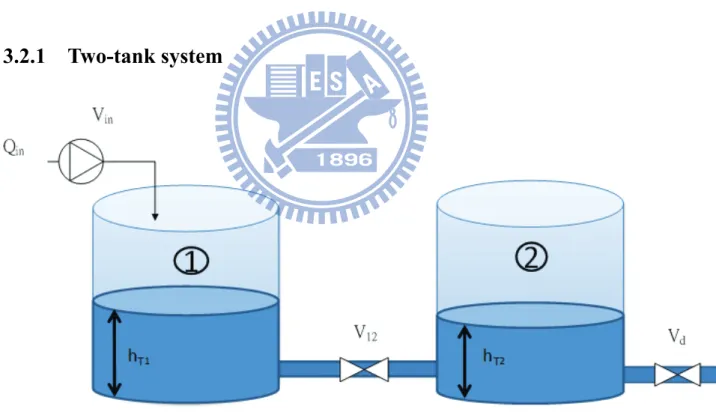
3.2.1 Two-tank system . . . 22
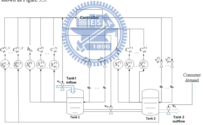
3.2.2 Proposed system with controller . . . 23
3.2.3 Dynamic model . . . 24
Chapter 4 Implementation 27 4.1 Linearized system . . . 27
4.1.1 Discrete time system . . . 30
4.2 Model predictive control . . . 30
4.2.1 Augmented model with embedded integrator . . . 30
4.2.2 Model predictive . . . 31
4.2.3 Optimization . . . 33
4.3 MPC with control constraints . . . 35
4.3.1 Constraints on control variables . . . 35
4.3.2 Hidreth's quadratic programming procedure . . . 36
4.4 Disturbances . . . 39
4.4.1 Inflow water quality . . . 39
4.4.2 Consumer water demand . . . 40
Chapter 5 Simulations 42 5.1 System model . . . 42 5.1.1 Preliminaries . . . 42 5.2 Simulations . . . 43 5.2.1 Nonlinear system . . . 43 5.2.2 Linear system . . . 45
5.3 Simulations with MPC . . . 48
5.3.1 MPC control with reference input . . . 49
5.3.2 Control without constraints . . . 50
5.3.3 Control with constraints . . . 52
5.4 Disturbances . . . 55
5.4.1 Time-variant inflow water quality . . . 55
5.4.2 Consumer water demand . . . 56 Chapter 6 Conclusion and Future Work 63
List of Figures
1.1 general architecture of control systems . . . 2
2.1 Water treatment process [1] . . . 7
2.2 Topology of water network . . . 8
2.3 Schema of open-loop water system . . . 12
2.4 Schema of close-loop water system . . . 13
3.1 simplified one-tank system schematic diagram . . . 18
3.2 Two-tank System . . . 22
3.3 general architecture of control systems . . . 23
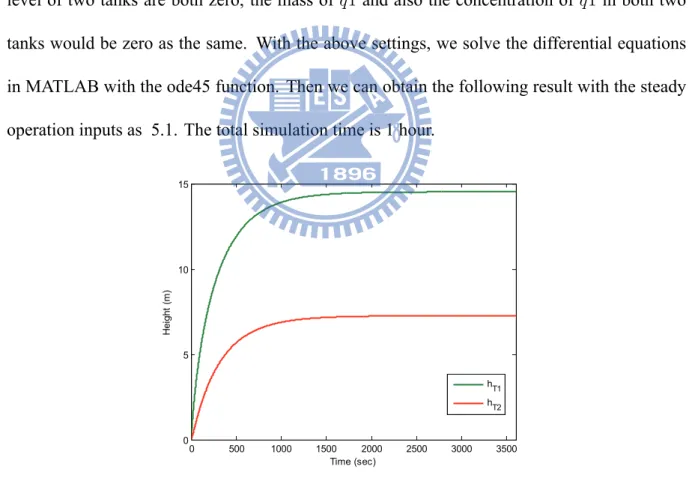
5.1 Nonlinear model: water level . . . 43
5.2 Nonlinear model: mass of q1 in tank 1, pipe and tank 2 . . . 44
5.3 Nonlinear model: concentration of q1 in tank 1 and tank 2 . . . 44
5.4 Water level . . . 50
5.5 Concentration of q1 in tank 1 and tank 2 . . . 51
5.6 Manipulated variables uvinand uv12 . . . 51
5.7 Manipulated variables uT 1 q1 and uT 2q1 . . . 52
5.8 Control with constraints: water level . . . 53
5.9 Control with constraints: concentration of q1 in tanks . . . 54
5.10 Control with constraints: manipulated variables uvinand uv12 . . . 54
5.11 Control with constraints: manipulated variables uT 1 q1 and uT 2q1 . . . 55
5.12 Control with quality disturbance: water level in tank 1 and tank 2 . . . . 56
5.13 Control with quality disturbance concentration of q1 in tank 1 and tank 2 . 57 5.14 Control with quality disturbance: manipulated variables uvinand uv12 . . 57
5.15 Control with quality disturbance: manipulated variables uT 1
q1 and uT 2q1 . . . 58
5.16 consumer demand . . . 58 5.17 control values to vd . . . 59
5.18 Control with demand disturbance: water level in tank 1 and tank 2 . . . . 60 5.19 Control with demand disturbance: concentration of q1 in tank 1 and tank 2 60 5.20 Control with demand disturbance: manipulated variables uvinand uv12 . . 61
5.21 Control with demand disturbance: manipulated variables uT 1
Chapter 1
Introduction
1.1
Process control system
Control systems are computer-based systems that monitor and control physical processes. These systems represent a wide variety of networked information technology system connected to the physical world. Depending on the applications, these control systems are also called Process Control System (PCS) , Supervisory Control and Data Acquisition (SCADA) systems,or Cyber-Physical Systems(CPS).
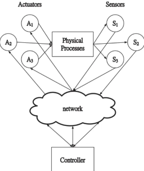
PCSs are usually composed of sensors, actuators, controllers and physical processes. The general architecture of PCS is shown as Figure 1.1. Sensors would monitor the status of the physical processes and the controller would send the control commands according to the in-formation from sensors to actuators to control the physical processes. Sensors and actuators communicate with controllers through networks.
PCS provides us a more powerful and flexible domination of the distributed collaborative works which are connected together by the network. With PCSs, we can supervise and adjust the physical processes remotely. The information about the physical system will be updated through the network to the control center. The physical processes are fully controlled by the central controller. The control center is the only authorized controller that give main control commands to the physical system.
őũźŴŪŤŢŭġ őųŰŤŦŴŴŦŴ ŔIJ ŔĴ Ŕij łij łĴ łIJ ůŦŵŸŰųŬ ńŰůŵųŰŭŭŦų łŤŵŶŢŵŰųŴ ŔŦůŴŰųŴ
Figure 1.1: general architecture of control systems
PCSs can be applied to a variety of critical infrastructures, like the electric power grid, factories and refineries, oil and gas pipelines and water infrastructures. We use PCSs to manage power systems to maintain successful and reliable system operation. The system is operated to meet the market requirements and also to control the power flowing properly over the network. Industrial plants such as chemical plants control their manufacture process to maintain their product rates and preserve the process environment. The water treatment systems utilize the PCSs to supervise the water purification process.
According to the appliance of PCSs, these systems are mostly safety-critical. Any damage on the system or unstable of the system would make great impact on the public or on the industry. With the safety-critical property of PCSs, we want to protect the control systems from being attacked.
To keep the system stable and safe, more and more mathematical modules and simulations of the PCS are investigated. We generate mathematical models to describe the physical process practically. Then apply the model in the simulation to simulate how the real physical system act with the conducted control commands accurately. Other interesting topics in PCS field including cyber-attack, optimization, and automatic system control.
• Cyber-attack
Nowadays the controllers and physical systems are getting more and more complex and independent. The essential constituents of PCSs such as the controller, sensors, and actu-ators transmit information through the network. The tightly network connected properties of control systems make PCSs vulnerable to the cyber-attacks. The main goal of attackers is to make the physical processes unstable. For cyber attacks, attackers could achieve these by making wrong control input commands or making bad sensor outputs. And these at-tacks could be realized by two ways, the first is to compromise sensors or actuators and the second is to make denial of service (DoS) attacks on the way of network communication between sensors and the controllers or the controllers and actuators[2]. Actually, system stability is mainly affected by the control commands. Bad control commands would lead the system to the states against the real situations of the physical system,[3].
The cyber security issue about the chemical plant is concerned and an anomaly detection system is proposed in [4]. Unauthorized assessment to the control center network of a power system is issued and an analytical framework to quantify the system vulnerability is proposed in [5].
• Optimization
PCSs are usually composed of a large number of elements which require energy to be driven and function. Furthermore, we desire to make the best use of resource to avoid unnecessary consumption. So concerning about the cost and effect, we aim to control the PCSs efficiently. We want to compute control commands to reach desired control strategies with the lowest cost and also achieving certain performance goals. The optical control assist the system with generating control strategies ahead of time to guarantee good performance of the control system. The optimization topics of the system operations are
developed in different applications of PCSs. For different areas, the problems requiring optical control are also different.
Optical control in water networks deals with the specific needs, such as minimization of supply and pumping costs, maximization of water quality, pressure regulation for leak prevention, etc. The optical control simulation of pump station operation is discussed in [6].
• Automatic system control
In the past, manual control is very common in PCS. The operation of the control system partially depends on the experience of the operators. However, the structure of PCS is get-ting more complicated and huge. The physical process system is decentralized in different places, the central control center will dominate the main control commands. Automatic system control is developed to assist controller decide the appropriate control signals to actuators. Also, different models for simulating variate functionality and fields are inte-grated together to help the operators compute the most adequate control commands, [7].
In this paper, we discuss one of applications of PCS, water system. Safe and high-quality water is required to the public. The issues of water quality and treatment are getting notice in recent years since the change of the weather and the higher requirement of clean water. In this paper, we propose a model to simulate the water system. And apply feedback control algorithm to control the water quality and hydraulic dynamic.
1.2
Synopsis
The thesis is organized as follows. The related background and studies of water system and the control algorithm will be introduce in Chapter 2. The system model will be proposed
in Chapter 3. The design method of controller will also be introduced in Chapter 4. We will examine the designed controller and the proposed model with simulations in Chapter 5. In the end, we conclude the thesis in Chapter 6.
Chapter 2
Background
2.1
Water system
Generally, water system could be divided into two part, water treatment systems and water distribution systems. Water treatment remove the undesired substances in raw water and main-tain expected water quality at outlet of the system. Water distribution system insure the delivery of high-quality water and steady supply to end-user.
2.1.1
Water treatment
In real life, we process the raw water into the water system to obtain clean and drinkable water. Several procedures are functioned in water system. The main water purifying process includes flocculation, precipitation, filtration and disinfection. The architecture of a typical water treatment system is shown as Figure 2.1. By means of these processes, the undesired chemicals, materials, and biological contaminants would be removed from raw water.
Procedures in water system are for different purposes. Flocculation is a process which re-moves turbidity or color of water. In this process, we aim to make the suspended solids in raw water form bigger particles. Most of the time, some chemicals will be injected to hasten the procedure. Then water will enter the procedure called precipitation. Tanks of this procedure are big and with slow flow. In this procedure, the bigger particles that form in the previous
Figure 2.1: Water treatment process [1]
procedure will settle since the slow water flow. Next procedure is called filtration. The remain-ing suspended particles will be filtered and removed. Last, we need to disinfect the water to decrease the risk of pathogen exposure to human. Also, at the disinfection procedure, chemicals are always necessary to be utilized [8].
2.1.2
Water distribution network
Water leaving water treatment will enter water distribution system to be delivered to end-user. Water distribution system aims to maintain water quality under the long distance and time for delivering water. Furthermore, water distribution system should also guarantee the uninterrupted supply of water.
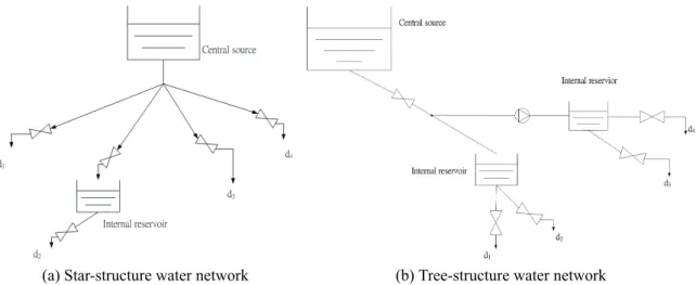
Generally, water distribution system is composed of actuators, pipes, and tanks. The topol-ogy affects the operation of the elements in water distribution system. Figure 2.2 shows some examples of topology of water distribution system [6]. Figure 2.2a shows a star-structure wa-ter network. The direction of wawa-ter flow is obvious. Usually, the central source is one large source to supply water to other consuming nodes. Figure 2.2b shows the tree-structure of water network. Tree-structure also contains a large reservoir for preserving water and supply water to the consumer nodes or internal reservoirs. The sense of the flows is defined, from source to the demands.
(a) Star-structure water network (b) Tree-structure water network
Figure 2.2: Topology of water network
For different topology, the control scenarios may be varied. But the control goal will stay the same, to deliver clean, qualified water and steady supply is the main purpose for controlling water distribution system.
2.2
Water quality
There are numerous factors when we evaluate the water quality. The factors include tur-bidity, concentration of residual chlorine, pH, temperature, etc.. Generally, Water quality is determined by three basic assessment, physical assessment, chemical assessment and biological assessment [9]. Qualified water should be colorless, tasteless and sterile. Physical assessment is the standard for the appearance and the taste of water; Chemical assessment is the standard for the dissolved chemicals in water; and the biological assessment is the standard for the biological contaminants in water, such as bacteria.
• Physical assessment
Physical assessment includes the limitation of turbidity, temperature, and odor etc.. Here we consider more about the factor that influences the appearance and the color of water, the turbidity. Turbidity is the measurement of the scattering degree of the suspended materials
toward light in water. There are several kinds of suspended materials in water, such as clay, organic or inorganic colloid, and plankton etc. [10]. Most of the time, the suspended solids which cause turbidity are harmless. However, these solids in water would protect pathogens from being disinfected and also decrease the possibility of raw water to be processed. If the turbidity of raw water is higher than the standard, the raw water cannot be treated directly.
• Chemical assessment
Chemical assessment includes the residual chlorine, heavy metals, orthophosphates etc.. The concentration of these chemicals in water has a great impact on the palatability of water. For example, chlorine is the most common disinfectant in water industry, be-cause of its low cost and high effectiveness of disinfection. Chlorine mixed with water forms hypochlorous acid and hypochlorite ions. These elements generated from chlo-rine are called effective residual chlochlo-rine. They are the chemical elements with powerful oxidizing properties. However, high concentration of chlorine in water may not reduce pathogen exposure effectively and even overreact with the organic compounds to produce by-products which may be harmful for human. Hence, the dose of disinfectant must be enough to achieve sufficient disinfection of the water, but not too much to produce exces-sive by-products. Appropriate control of the concentration of the concentration of these chemicals is very important.
• Biological assessment
Biological assessment is mainly the limitation of the concentration of different kinds of organisms in water. High concentration of organisms such as bacteria, Escherichia coli, cryptosporidium etc., may be risky to human health. We usually utilize the chemicals to reduce the concentration of these organisms in water. The chlorine which discussed
before is the common one to disinfect.
To meet these quality standards, chemicals are very common to be utilized. For example, chlorine is usually used for disinfecting and coagulant for reducing the turbidity. The concen-tration chemicals should be ranged in the regulation, since the too much chemicals in water are also not appreciate.
In this paper, we consider the concentration of the chemicals in water as the major factors when we concern water quality. To control water quality to meet the end-user, concentration of the chemicals in water is what we concern and aim to control in the following work.
2.3
Water system with process control
To provide safe and drinkable water for end-user, adequate water treatment control is nec-essary. We intend to control the water system to approach the desired output of the system. For water treatment system, water suppliers want to control the hydraulic stability and also optimize each process of the treatments. For water distribution system, we want to control the system to supply steady quantity of water and qualified water.
2.3.1
Water treatment with process control
With controller to water treatment system, we aim to control the system to maintain water quality and meet time variant consumer demand for water. To control and understand more about the behavior of the water treatment system, simulators are developed to assist water suppliers to realize how systems react under different control strategies and situations [11]. The followings are some currently used simulators :
OTTER is coded in FORTRAN and developed by WRc. OTTER simulate the dynami-cal changes in raw water quality, flow and process operating conditions. OTTER assist the operators to analyze the disinfectants changes under different strategies, to study the effects of pH control on coagulation strategies, to predict the maximum throughput of a treatment works and to evaluating the monitoring strategies on a treatment works, etc.. OTTER is designed to be operated with friendly GUI interface for user [12].
• Stimela
Stimela models the environment of water treatment system developed by DHV Water BV and the Delf University of Technology [13]. Stimela especially focus on the analysis and simulating water quality. Stimela models of drinking water treatment processes calculat-ing the changes of water quality factors, such as pH, oxygen concentration etc.. Stimela also allows different models to be connected, hence the effects between each models could be evaluated.
• WatPro
WatPro is the water treatment simulator for predicting water quality based on specific treatment processes and chemical addition. WatPro provides analysis on steady water condition [11]. WatPro models the behavior of each treatment process and concern the dynamic of the chemicals in water. WatPro is easy for user to generate different water treatment topology [14].
Most of these simulators focus on different procedures of water treatment system. They simulate the behavior of flocculation, disinfection, sedimentation, etc.. Few of these simulators particularly emphasize on the control algorithm of water treatment system.
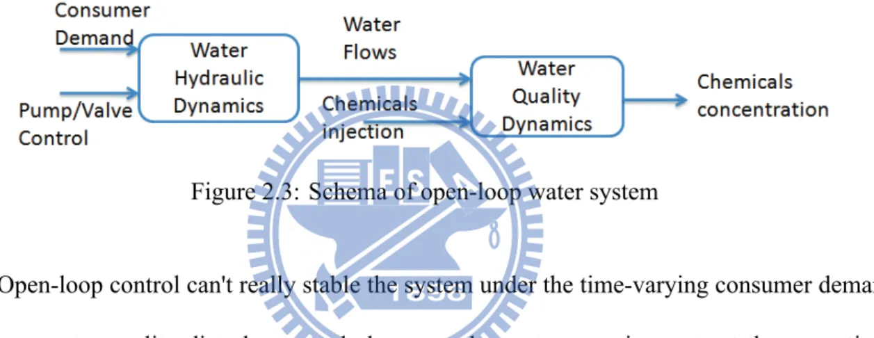
Most water systems use open-loop control to adjust the systems. For example, chlorine would be joined to the system at the beginning of the treatment, and then if the concentration of chlorine at output doesn't meet the standard, more chlorine would be added at the output position. The concentration of chemicals in water would be affected by the hydraulic dynamic of water, since the volume of water affects the concentration of chemicals strongly. The time-variant volume of water in water system would be a great factor to influence the water quality. Therefore, excessive chlorine might be injected at output and may cost more with open-loop control. The concept of open-loop control water system could be shown as Figure 2.3.
Figure 2.3: Schema of open-loop water system
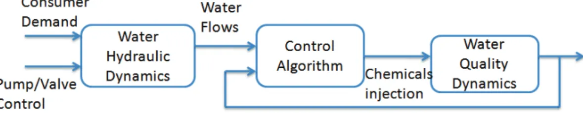
Open-loop control can't really stable the system under the time-varying consumer demand and raw water quality disturbance and also meet the system requirements at the same time. Hence, we want to use the idea of feedback control to balance the injection of chemicals and also the volume of water preserve in water system. The block diagram in Figure 2.4 shows the general idea of feedback control in water system. With feedback control, the control center monitor the output of the system and adjust the control command with the feedback result. With the real-time monitoring and adjusting, the outputs of the system are expected to meet the desired values.
The most difference between open-loop control and feedback control in water system is that feedback control traces the output of the system and then adjusts the control signal to lead the system to approach the desire output. In this paper, we design the feedback controller with model predictive control algorithm.
Figure 2.4: Schema of close-loop water system
2.3.2
Water distribution with process control
The model of water distribution system is developed in past decades. One of the most important and common issues of water distribution system is water quality of the system. Clean water leaving the water treatment system may fall out of the standard in the delivering process. Since we usually want to keep a detectable concentration of some specific chemicals in water, such as chlorine, the reaction property of these chemicals itself might affect the concentration at consumer position after long delivering time.
Chlorine is widely used in water system to protect the potentially risk of pathogen from public. The concentration of residual chlorine could be consider as an dominated factor for water quality. The concentration of chlorine should be enough to achieve sufficient disinfection, but not too much to produce excessive by-products. Furthermore, chlorine in water will decay with time. To maintain an appropriate concentration of chlorine become one of the major problems in water distribution system.
Several models have been developed to study the changes of chlorine in water distribution system. In [15], a mass-transfer-based model is proposed to predict chlorine decay in drinking water distribution system. The model concerns the reaction between chlorine in water and pipe wall and also the decay rate of chlorine. An input-output model of chlorine transport in drinking water is proposed in [16]. A model tracing chlorine transport using a time-driven approach and evaluating chlorine decay in drinking water distribution system is mentioned in [17].
An general model to describe water quality is proposed in [18]. The model evaluates the changes of chlorine in water according to the dynamic property of water distribution system. Feedback control algorithm is applied to the model to meet the different position of end-user. In [19], adaptive control algorithm is utilized to control the water distribution system to meet the time-variant consumer demand and water quality.
In this paper, we focus on analyzing water treatment system. We consider only water treat-ment system as we treat-mention water system. We propose s system to model the water treattreat-ment system and apply feedback control to water system. In the proposed model, model predictive control is the control algorithm we apply to control the water system.
2.4
Model predictive control
Model predictive control, represented as MPC, is widely used in variety applications in PCS, such as chemistry plant [20], oil refineries etc.. MPC refers to a class of computer algorithms that compute a sequence of future manipulated control signals to optimize the future behavior of system outputs. The optimization is performed within a limited time window which is a slide window for predicted system states and manipulated control signals. At each control interval, MPC slides the time window to compute the next time horizon control signal. By giving the plant information at the start of the window, MPC utilizes an explicit process model to generate the optimized control signals [21].
In this paper, we choose MPC as the algorithm for designing controller for the proposed system. The followings are two main advantages for determining MPC as the design law.
2.4.1
Real-time optimization
MPC is a method to compute the most appropriate control signal to lead the output of the system to desired states on-line. For each sampling time, MPC compute the control signals for next sampling time with current information of the plant. Hence, with MPC, the controller will adjust to meet the dynamic behavior of the plant and lead the system to achieve desired outputs. The on-line optimized ability of MPC is one of the impotents reasons why we choose MPC as the control algorithm in this paper.
When computing the optimized control signals for PCSs, we conduct the cost function and try to minimize the cost function to derive the optimal solutions. Least quadratic regulator (LQR) is also a popular method using the cost function to find the optimal solution for multivariable control system. The major difference between MPC and LQR is that the MPC uses a moving time horizon window to derive optimized solutions and LQR solve the problem with a fixed time window. The moving time horizon window enables MPC compute real-time optimized control signal [22].
2.4.2
Design with constraints
As we discussed before, one of the components of PCSs are actuators. Most of the actuators have some limitation according to the physical property in real life. For example, we might use valve to control the open ratio of a pipe. The control signal for this valve could not be excessive large or negative. The maximum open degree of the pipe is one hundred percent, which means completely opened; thus control signal to this valve should also be maintained in this range.
For operational constraints, we must address the concept of the constraints of control signal when designing controller for the PCS. MPC is a control method that is able to add the con-straints to control variables. MPC can handle both soft concon-straints and hard concon-straints [23] in
Chapter 3
System model
Generally, a water system may be composed of tanks, pipes, pumps, and valves. Tanks and pipes are two major components that retains water. Pumps and valves are the components used to control the direction and volume of water flows. In a water system, water traverses from tank to tank through pipes. Pipes link tanks where water retained and reacted. In this paper, a tank, connected by pipes, is then considered as a basic unit in a water system. This section explains the traditional single tank-based water system to overview a water system.
3.1
A single tank-based water system
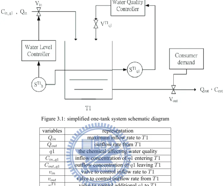
An single tank water system is composed of one tank, several sensors, controllers and valves. Figure 3.1 illustrates an example of a single tank-based water system. In the figure,
Cin q1and Qinstand for the input volume and quality of water. To fulfill consumers' demands,
two sensors ShT 1and Sq1T 1are used to sense the water level and water quality of the tank 1. The sensing data reported by the sensors are forwarded to the corresponding controllers. Conse-quently, the controllers control the valves vin and vqlT 1 to maintain the quality of water at the
level configured according to consumers' demands.
The system consists of a single tank reserving the water from external resource and out-putting the water flow. The tank is denoted as T 1. The variables in Figure.1 are defined in Table.3.1.
Figure 3.1: simplified one-tank system schematic diagram variables representation
Qin maximum inflow rate to T 1 Qout outflow rate from T 1
q1 the chemical affecting water quality
Cin q1 inflow concentration of q1 entering T 1 Cout q1 outflow concentration of q1 leaving T 1
vin valve to control inflow rate to T 1 vout valve to control outflow rate from T 1 vT 1
ql valve to control additional q1 to T 1 ShT 1 sensor for detecting water level of T 1
ST 1
q1 sensor for detecting concentration of q1 in T 1
Table 3.1: Notations of single tank system in Figure.1
In this single tank-based water system, the system states that we concern about could be mainly divided into two categories, water level and water quality.
• Water level
vinis controlled by water level controller to regulate the water inflow rate Qin. The sensor ST 1
h monitors the water level of T 1 and send back the information to water level controller.
The controller would adjust the control signal to valve, vinto control the input flow rate.
flow rate. Water level of T 1 is also impacted by the output flow rate, which is controlled by vout.
The output flow rate is controlled by vout. The control value of vout effects the cross
sectional area of the output pipe of T 1. The control strategy of vout is influenced by
consumer water demand. Higher consumer demand refers to greater control value to vout
and vise versa.
• Water quality
Cin q1 affects the concentration of q1 in T 1 directly. q1 in inflow combine with q1 in T 1 immediately. The sensor Sq1T 1 senses the concentration of substance q1 in T 1 and then the water quality controller will compute the control signal to vT 1
ql depending on the
information provided by Sq1T 1. The valve vT 1ql effect the dosage of the chemicals added to
T 1. The more q1 is added to T 1, the higher value the Sq1T 1would sense.
In this paper, we focus on construct the environment for describing the behavior of the water treatment process. We conduct some mathematical formulations to describe the dynamical behavior of the water system.
3.1.1
Mathematical formulation
We use mathematical formulations to describe the hydraulic behavior in water tanks and pipes and the features of dissolved elements that affect water quality.
• Hydraulics model
For components preserving water in water system, the change of water level of these com-ponents could be obtained by the relation between water inflow and outflow. The variation of the water level equals to the difference between the total water volume entering into
the tank or pipe and the summation of the water leave the tank or the pipe. The following equation describes the differential changes in water level of a water tank.
˙
hT =
(Σ(Qin)− Σ(Qout) AT
(3.1)
where hT is the height of the water level in water tanks, Qinis the input flow rate (volume/
time) from external source, Qout is the output flow rate discharged water from the tank,
and AT is the cross sectional area of the tank.
Assume that the flow obeys Torricelli's Law [24], the outflow rate could be derived as follows,
Qout= Apup
√
2g(hhigh− hlow) (3.2)
We assume that water flows from the position with hight hhighto the place with hight hlow. g is the gravitation acceleration. Apis the cross sectional area of the output pipe and upis
the control parameter that control the open ratio of the output valve. From above equation, we can understand the relation between the outflow rate and water level of the tank.
• Quality model
Since the quality we discussed in this paper is the concentration of the chemicals in wa-ter, we model the variation of the concentration of the dissolved substances in water for solving water quality issues. We assume that the dissolved substances are completely and instantaneously mixed either in tanks or in pipes. The concentration of the dissolved sub-stance equals to the total mass of the subsub-stance divided by the total volume of the water in pipes or in tanks. The total mass of a certain substance at current time t equals to the sum of the mass of the dissolved substance in the tanks or pipes at time t−1 and the difference between the sum of the input mass of the dissolved substance at time t and the sum of the
output mass of the substance at time t. The concentration formulation could be computed as following,
C(t) = ΣQin(t)Cin(t)T − ΣQout(t)C(t)T + V (t− 1)C(t − 1)λ
ΣQin− ΣQout+ V (t− 1)
(3.3)
where C(t) is the concentration of dissolved element at time t, Qin(t) is the input flow
rate from external resource at time t, Qout(t) is the output flow rate, V (t−1) is the volume
of water stayed in storage facilities, and λ is the decay rate of the dissolved substance. The reaction rate of the dissolved substances could be described as following [25],
dC
dt = KbC
n (3.4)
Kbis the reaction coefficient of the substance and Kbis varied with different element. The
substances grow with time if Kbis greater than zero, and the substances decay with time
if Kb is less than zero. The larger the Kb is, the faster the reaction would be. C denotes
the concentration of the dissolved substance in water. n is the reaction order. The reaction order is different with different properties of substances.
Now consider more about the variation of the concentration of the chemicals in a very small time period, hence we aim to derive the differential formulation to describe the change in concentration. For a variable-level tanks or pipes, the variation of concentration could be represented as the variation of the mass of the substance, [26].
d(CV )
dt = QinCin− QoutC + KbCV (3.5)
where C is the fully mixed concentration of the substance and V is the volume of the water in tanks or pipes. The above equation describes the change in mass of the dissolved substance in water. The change in mass of the substance equals to the variation between the mass entering the container and those leaving the container and plus the reaction rate of the substance itself.
3.2
Proposed system
We can consider the water treatment process as the process that water transport from one tank to another tank, and proceed different physical or chemical reaction in each tank. The factors that we measure as the standard for water quality would vary according to different treatments in each tanks and the change of water volume. Namely, water quality is impacted by water processing action in those tanks before current tank where tank quality is measured as well. Hence, the two tank system is proposed to meet the dynamic of the water hydraulic properties and the situation of the interaction between any connected two tanks. The two-tank water system as Figure 3.2.
3.2.1
Two-tank system
Figure 3.2: Two-tank System
There are two tanks in the proposed model, tank 1 and tank 2. There is also one pipe to connect these two tanks. External water resource enter the system from the input pipe of tank 1, denoted as Qin. Qinis the only input node that import water from outside of the system. The
water quality of a specific substance. We assume that the concentration of the substance, which is denoted as q1, will affect the water quality. There is only one outlet of the two tank system, which is at tank 2. The output pipe of the tank 2 is the only one place for water leaving the two tank system.
3.2.2
Proposed system with controller
To control the water level and quality issue of the two tank system, we modify the above two tank system with controller to command the control signal to the valves. With the controller, we expect the system will achieve the states that we desire. The two tank system with controller is shown as Figure 3.3.
Figure 3.3: general architecture of control systems
In Figure 3.3, there are numerous sensors to monitor system states. Sensors for monitoring water level in tanks are denoted as STi
h , where i = 1, 2 refers to tank 1 and tank 2. For example, ST 1
h represent to the information about the water level of tank 1. Sensors for sensing the water
quality could be represented as STi
refers to the substances that we concern about. For instance, ST1
q1 represent to the information
that sensor read about the concentration of solute q1 in tank 1. The water quality at the output node will be sensed by ST2b
qj , where j = 1, 2...n refers to the different water quality factors. The
sensor will read the concentration of qj at the output pipe of tank 2 and send the information back to the controller.
There are also lots of valves for the controller to control the system to modify the system states. Valves for adding chemicals could be represented as vqjT i, where i = 1, 2 refers to tank 1 and tank 2 and j = 1, 2...n refers to the substances that we concern about. For instance, vT 1 q1
represents the valve to control the dosage of q1 injected to tank 1. Valve vin is for controlling
the input flow rate of importing resource. The value of vindetermine the open ratio of the pipe;
the value to vin proportions to the inflow rate. The valve, v12, is to control the water flow from
tank 1 to tank 2. Still, the value of v12proportions to the opened cross sectional area of the pipe
between two tanks. And there is a valve, vd, to control the output flow from tank 2. The control
value of vddepends on the consumer water demand. If the water consumption is heavy, then vd
should be more open relatively, and vise versa.
For the proposed two tank system, we aim to maintain the water level and the water quality. The water level should lower the hight of the tank and also higher than a minimum hight. The minimum value of hight is designed to meet the consumer water need, since we have to preserve certain amount of water in the tanks to handle the unpredictable changes of consumer demands.
3.2.3
Dynamic model
We apply the mathematical equations to characterize the features of the proposed model. We can derive the dynamic model of the proposed system. The dynamic model is discussed separately as the followings, the water hydraulics and water quality .
• Water hydraulics
The dynamic equations could be obtained as follows, ˙ hT 1 = uvinQin− uv12Ap √ 2g(hT 1− hT 2) AT 1 (3.6) ˙ hT 2 = uv12Ap √ 2g(hT 1− hT 2)− udAp √ 2ghT 2 AT 2 (3.7)
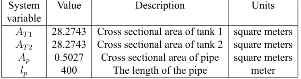
hT 1and hT 2denote the water level of tank 1 and tank 2, respectively. Qin (L/sec) is the
maximum inflow rate of water entering into tank 1. Ap is the cross sectional area of the
pipe. AT 1and AT 2are the cross sectional area of the tank 1 and tank 2.
uvinis the control value suggesting the status of valve vinof the input pipe of tank 1. The
value of uvin is 1 indicating the valve is completely opened and 0 meaning the valve is
fully closed. The value of valve will affect the flow rate of the input pipe of tank 1. uv12is
the control value suggesting the status of valve v12between tank 1 and tank 2. Similarly,
value 1 for u12indicates open and zero means close. The value of valve will affect the
flow rate from tank 1 to tank 2.
The dynamic model of water quality is described as follows, ˙ MT 1 q1 = uvinQinCin q1− MT 1 q1 AT 1hT 1 Apuv12 √ 2g(hT 1− hT 2)− Kq1Mq1T 1+ u T 1 q1 (3.8) ˙ Mq1p = M T 1 q1 AT 1hT 1 Apuv12 √ 2g(hT 1− hT 2) − M p q1 Vp Apuv12 √ 2g(hT 1− hT 2)− KMq1p (3.9) ˙ MT 2 q1 = Mq1p Vp Apuv12 √ 2g(hT 1− hT 2) − Mq1T 2 AT 2hT 2 udAp √ 2g(hT 2)− Kq1Mq1T 2+ u T 2 q1 (3.10) Cq1T 1 = M T 1 q1 AT 1hT 1 (3.11) Cq1p = M p q1 V p (3.12) Cq1T 2 = M T 2 q1 AT 2hT 2 (3.13)
Mq1T 1, Mq1p and Mq1T 2denote the mass of q1 in tank 1, the pipe and tank 2, respectively. Cin
is the concentration of q1 of the inflow resource to the tank 1. Vp is the volume of water in the
pipe between tank 1 and tank 2.
We attempt to add more q1 in water to maintain the water quality.uT 1q1 and uT 2q1 are two control variables for controller to control the injection of q1 to tank 1 and tank 2. uT 1
q1 and uT 2q1 denote
the value for the mass of q1 increasing to tank 1 and tank 2, respectively. uT 1q1 and uT 2q1 should be greater than zero, since the mass of additional q1 would always greater or equal to zero.
Chapter 4
Implementation
In this chapter, we discuss the method to design the controller for the proposed model in chapter 3. We will consider to compute the linear model of the water system first to design the controller. Then we will utilize MPC to design an appropriate controller and consider the constraints to the control signal into designing.
4.1
Linearized system
To design the controller of the proposed model, we compute the linearized model to describe the behavior of the system under some specific linearized range, which is defined as nominal points. With the linearization theorem[27], we will get the state-space equations as (4.1),(4.2) with the system variables as (4.3) based on the equations of system model ((3.6) (3.13)).
_
x = Acx + Bcu (4.1)
y = Ccx (4.2)
with the states, control variables and output variables
x = hT 1 hT 2 MT 1 q1 Mq1p MT 2 q1 , u = uvin uv12 uT 1 q1 uT 2 q1 , y = hT 1 hT 2 CT 1 q1 CT 2 q1 (4.3)
By the linearization theorem, we get the system matrix, Ac, Bc and Cc. The elements of Ac
could be represented as the followings,
A11 = −A puv12 AT 1 g √ 2g(hT 1− hT 2) A12 = Apuv12 AT 1 g √ 2g(hT 1− hT 2) A13 = 0 A14 = 0 A15 = 0 A21 = ASpuv12 AT 1 g √ 2g(hT 1− hT 2) A22 = Apuv12 AT 1 g √ 2g(hT 1− hT 2) −udApg AT 2 1 2ghT 2 A23 = 0 A24 = 0 A25 = 0 A31 = MT 1 q1 Apuv12 AT 1hT 1 ( 1 hT 1 √ 2g(hT 1− hT 2)− g √ 2g(hT 1− hT 2) ) A32 = MT 1 q1 Apuv12 AT 1hT 1 g √ 2g(hT 1− hT 2) A33 = −A puv12 AT 1hT 1 √ 2g(hT 1− hT 2)− Kb A34 = 0 A35 = 0 A41 = MT 1 q1 Apuv12 AT 1hT 1 (−1 hT 1 √ 2g(hT 1− hT 2)− g √ 2g(hT 1− hT 2) )− M T 2 q1 Apuv12g Vp √ 2g(hT 1− hT 2)
A42 = −MT 1 q1 Apuv12g AT 1hT 1 √ 2g(hT 1− hT 2) − M p q1Apuv12g Vp √ 2g(hT 1− hT 2) A43 = Apuv12 AT 1 √ 2g(hT 1− hT 2) A44 = Apuv12 Vp √ 2g(hT 1− hT 2)− Kq1 A45 = 0 A51 = Mq1pApuv12g Vp √ 2g(hT 1− hT 2) A52 = −Mp q1Apuv12g Vp √ 2g(hT 1− hT 2) + M T 2 q1 Apud AT 2hT 2 ( 1 hT 2 √ 2g(hT 1− hT 2)− g √ 2ghT 2 ) A53 = 0 A54 = Apuv12 Vp √ 2g(hT 1− hT 2) A55 = Apud AT 2hT 2 √ 2ghT 2− Kb
where Aij represents for the ijth elements in Ac
And Bc and Ccare
Bc = Qin AT 1 −Ap AT 1 √ 2g(hT 1− hT 2) 0 0 0 Ap AT 2 √ 2g(hT 1− hT 2) 0 0 QinCin −MT 1 q1Ap AT 1hT 1 √ 2g(hT 1− hT 2) 1 0 0 −M T 1 q1Ap AT 1hT 1 √ 2g(hT 1− hT 2)− −Mp q1Ap Vp √ 2g(hT 1− hT 2) 0 0 0 −M p q1Ap Vp √ 2g(hT 1− hT 2) 0 1 Cc = 1 0 0 0 0 0 1 0 0 0 −MT 1 q1 AT 1h2T 1 0 1 AT 1hT 1 0 0 0 −M T 2 q1 AT 2h2T 2 0 0 A 1 T 2hT 2
These is the system model in algebra form. We will apply number to describe the practical situation in the chapter 5.
4.1.1
Discrete time system
We usually use digital computer to implement controllers. Hence, design the controller based on the discrete time model is inevitable. The methods of converting the continuous time system model into discrete time is discussed in [27]. There are also functions in MATLAB to digital the continuous time model. The state-space mode in discrete time would be represented as follows,
x(k + 1) = Adx(k) + Bdu(k) (4.4)
y(k) = Cdx(k) (4.5)
In the following controller design, we will use the discrete time model as the system model of the plant.
4.2
Model predictive control
We use model predictive control method to control the two-tank system. Utilize the benefit of feedback control to trace the output of the system and use MPC to predict the future behavior of the system. With the controller designed with these methods, we expect the proposed system can achieve the desired performance.
4.2.1
Augmented model with embedded integrator
Before we apply the MPC algorithm to compute the controller for the proposed model, we try to add the integrator into the space-state equation. The integrators could help the plant to reach the zero error states compare with the reference input.
The basic idea of merging integrators into the system model is shown as followings. We first construct the difference equation of the system states and control signals. Thus, we can
obtain
∆x(k + 1) = x(k + 1)− x(k)
= Ad(x(k)− x(k − 1)) + Bd(u(k)− u(k − 1)) (4.6)
∆u(k + 1) = u(k + 1)− u(k) (4.7) Then apply the above equations into the output states. The outputs of the system can be derived as follows,
y(k + 1)− y(k) = Cd(x(k + 1)− x(k))
= Cd∆x(k + 1)
= Cd(Ad∆x(k) + Bd∆u(k)) (4.8)
Putting together the equations (4.6),(4.7) and (4.8) will lead to the following state-space model.
xn(k+1) z }| { ∆x(k + 1) y(k + 1) = A z }| { Ad oT CdAd I xn(k) z }| { ∆x(k) y(k) + B z }| { Bd CdBd ∆u(k) (4.9) y(k) = [ o I ] | {z } C ∆x(k) y(k) | {z } xn(k) (4.10)
where I is the identity matrix and o is zero matrix. In our case, the size of the identity matrix is 4× 4 and the size of o is 4 × 5. We can consider the above augmented model as the new state-space equation of the system. And we will design the controller for the plant based on this augmented model.
4.2.2
Model predictive
We use model predictive control to predict Np states of the system based on current system
predict Np states at time ki+ 1, ki + 2, ...,ki + Np. From the state-space equations (4.9) and
(4.10), we can induce following equations,
x(ki+ 1|ki) = Ax(ki) + B∆u(ki) x(ki+ 2|ki) = Ax(ki+ 1|ki) + B∆u(ki) = A2x(ki) + AB∆u(ki) + B∆u(ki+ 1) x(ki+ Np|ki) = ANpx(ki) + ANp−1B∆u(ki) + ANp−2B∆u(ki + 1) + . . . + ANp−NcB∆u(k i+ 1)
With the predicted states, we can also derive the predicted output of the system. The predicted output is computed based on the predicted Npsystem states, hence we can also get Nppredicted
output based on the current system states, which could be shown as follows.
y(ki+ 1|ki) = CAx(ki) + CB∆u(ki)
y(ki+ 2|ki) = CA2x(ki) + CAB∆u(ki) + CB∆u(ki+ 1)
y(ki+ Np|ki) = CANpx(ki) + CANp−1B∆u(ki) + CANp−2B∆u(ki+ 1)
+ . . . + CANp−NcB∆u(k
i+ 1)
We can represent the above equations into vector form as followings,
where F = CA CA2 CA3 ... CA(Np) , Φ = CB 0 0 ... 0 CAB CB 0 ... 0 CA2B CAB CB ... 0 CA3B CA2B CAB ... 0 ... CA(N p− 1)B CA(Np− 2)B CA(Np− 3)B ... CA(Np − Nc)B and Y = [
y(ki+ 1|ki) y(ki+ 2|ki) y(ki+ 3|ki) ... y(ki+ Np|ki)
]
∆u = [
∆u(ki+ 1|ki) ∆u(ki+ 2|ki) ∆u(ki+ 3|ki) ... ∆u(ki+ Nc− 1|ki)
]
In our case, we compute the matrix, F, whose size is 40× 9 and Φ sizing 40 × 12. The size of F and Φ will change according to the value of Np, Nc and the original size of the system matrix.
Equation (4.11) shows the relation between control signals and system states based on the MPC algorithm. The output of the system Y also includes the predicted future system outputs based on the predicted system states and control variables. We aim to control the current system outputs and future outputs to approach out expectation.
4.2.3
Optimization
We want to design a controller to drive the system to approach the desire states. The desire states are usually the reference input to the system. That is, we aim to make the system outputs equal to the reference input. The two tank system is a multivariable system; therefore, we need to balance the impact of each control variables on the output variables. Focusing on one specific control variable and thus affecting on some certain outputs are not appreciate for our proposed
system. Thus, we use the cost function to help us to balance each control input signal to achieve the desire system states.
The cost function J is defined as
J = (R− Y)T(R− Y) + ∆uTQ∆u
= (R− F(xi))T(R− F(xi))− 2∆uTΦT(R− Fx(ki)) + ∆uT(ΦTΦ + Q)∆u (4.12)
where Y is the output Y in (4.11) and ∆u is the control variable in (4.11). x(ki) is the augmented
system state at control period, ki. R is the reference input to the system. Q is the adjustable
variable for designing the controller. The value of Q will affect the performance of the controlled system.
We aim to approach the system outputs to be identical to the reference inputs. Thus, we put (R−Y)T(R−Y) in cost function and try to minimize the difference between system outputs and
reference inputs. Since we want to control the water level of tanks and water quality in water treatment system, the severe transient response is not appreciate. For example, the water level should be under the capacity of the tanks. The severe transient response may lead the water level to be greater than the limitation. Thus, ∆uTQ∆u is added in cost function to adjust the
performance of the control system. With the added term, the behavior of the system is regulated by controlling the value of the control signal, u.
The cost function is computed based on the equation (4.11) and the augmented system model with state-space equations (4.9), (4.10). We want to minimize the cost function to find the optimal solution.
To minimize J, we take partial derivation of J as follows,
∂J
∂∆u = 0 (4.13)
control signal that minimize the cost function. The result of the derivative of the cost function J is shown as (4.14) ∂J ∂∆u =−2Φ T(R− Fx(k i)) + 2(ΦTΦ + Q)∆u (4.14)
From (4.13) and (4.14), we could get the optimal ∆u.
∆u = (ΦTΦ + Q)−1ΦT(R− Fx(ki)) (4.15)
The ∆u is the optimized control signal input to the plant.
4.3
MPC with control constraints
Because of the physical limitation of the actuators, such as valves, the control signal to valves should be ranged. The above optimized control signals are not limited; hence, the control value assigned to uT 1
q1, for example, might be less than zero. However, uT 1q1 represent the dosage
of q1 to tank 1; therefore, the control value of uT 1
q1 should be ranged to be greater than zero. We
discuss the constraints of control variables in the following sections.
4.3.1
Constraints on control variables
The values of the variables that we can control in the proposed system refers to the control signal sending to the valves in the system. The constraints of the valves could be represented as followings,
uminvin ≤ uvin≤ umaxvin uminv12 ≤ uv12 ≤ umaxv12 uT 1q1 min≤ uT 1 q1 ≤ u T 1 q1 max uT 2q1 min≤ uT 2 q1 ≤ u T 2 q1 max (4.16)
uvinis the value to control the open ratio of the input valve. uminvin is the minimum value of uvin
and umax
vin is the maximum value of uvin. uv12 is the value to control the open ratio of the pipe
between two tanks. umin
v12 is the minimum value of uv12 and umaxv12 is the maximum value of uv12.
These two control variables are both two variables for controlling the lifted degree of the valve to adjust the cross sectional area of the pipe. Since the value for these two variables is the open ratio of the valves, they are generally ranged between zero and one.
uT 1q1 is the value to control the dosage of q1 to tank 1. uT 1q1 min is the minimum value of uT 1
q1 and uT 1q1 max is the maximum value of uT 1q1. uT 2q1 is the value to control the dosage of q1
to tank 2. uT 2
q1 min is the minimum value of uT 2q1 and uT 2q1 max is the maximum value of uT 2q1.
The values assigned to these two control variables represent the mass of the dosage. Hence, the minimum value of these two variables are usually set to be zero.
4.3.2
Hidreth's quadratic programming procedure
We apply Hidreth's quadratic programming procedure to compute the optimized solution with constraints of the control input signal. For the Hidreth's quadratic programming procedure, the cost function Jdis defined as follows,
Jd = 2∆uTLTQcGxf+ ∆u(LTQcL + Qr)∆u (4.17)
= 2∆uTf + ∆uTE∆u (4.18) where ∆u is the manipulated variables. Qr is the input variable for adjusting the performance of the system. Qc = CTC and xf is the system states modified with augmented system states,
which could be represented as
where x(ki) is the system state of discrete time system and y(ki) is the system output of the
system at control period ki. r(ki) is the reference input at time ki. And G and L in (4.17) are
G = A A2 ... ANp (4.20) L = B 0 0 ... 0 AB B 0 ... 0 A2B AB B ... 0 ... ANp−1B ANp−2B ANp−2B ... ANp−NcB (4.21)
where A and B are system matrix of the augmented model. The cost function is subjected to constraints as (4.16). The constraint function can be computed as follows then,
− ∆uvin ≤ −∆uminvin
∆uvin ≤ ∆umaxvin −∆uv12 ≤ −∆uminv12
∆uv12 ≤ ∆umaxv12
−∆uT 1
q1 ≤ −∆uT 1q1 min
∆uT 1q1 ≤ ∆uT 1q1 max
−∆uT 2
q1 ≤ −∆u
T 2
q1 min
∆uT 2q1 ≤ ∆uT 2q1 max
Above equations can be represented as Acons∆u≤ b (4.23) where Acons= −I4×4 I4×4 , ∆u = ∆uvin ∆uv12 ∆uT 1 q1 ∆uT 2q1 , b = −∆umin vin ∆umax vin −∆umin v12 ∆umax v12 −∆uT 1 q1 min ∆uT 1q1 max −∆uT 2 q1 min ∆uT 2 q1 max (4.24)
Now we can utilize the Hidreth's quadratic programming procedure to compute the optimized solution of ∆u. H = AconsE−1Acons (4.25) K = b + AconsE−1f (4.26) xo = −E−1f (4.27) then ∆u = xo− E−1Aconsλ∗ (4.28)
where λ∗ is the convergence result of λ. And λ is
λm+1i = max(0, ωim+1) (4.29) with ωim+1 =− 1 hij [ki+ Σij=1−1hijλm+1j + Σ n j=i+1hijλmj ] (4.30)
where the scalar hij is the ijth element in the matrix H, and ki is the ith element in the
vector K. With numerous times of the computation of λ, λ will converge to a steady number, which is λ∗then. With the derived λ∗, we can get the optimal solution of ∆u.
4.4
Disturbances
The unknown consumer demand and inflow water quality are interpreted as disturbances for the two tank system. In previous design and implementation, we regulate the control signal for outflow and input water quality to be constant. Now we consider more about the alteration of outflow rate and inflow water quality. The continuous state space equations could be computed as follows,
_
x = Ax + Bu + Wcd (4.31)
where Wcis the disturbance matrix for the system and d is the disturbance signal.
We expected the proposed system with the designed controller would still be stable and controllable to achieve the desire states.
4.4.1
Inflow water quality
Inflow water quality may be varied due to the weather, the pollution at the raw water district, the temperature etc.. The weather might be a great influence on water quality. During the raining season, the turbidity of the water might be greater since rapid speed of the river or at raw water district since the pouring rain brings a great amount of substances into raw water. The unknown inflow water quality would be considered as disturbance to the system. Since we can not exactly predict the changes of the water quality of the inflow.
Cin q1, is a time-variant disturbance of the water system. The disturbance system matrix could be shown as follows, Wc = 0 0 uvinQin 0 0
and d here is the value of the inflow water quality, Cin q1.
4.4.2
Consumer water demand
The consumer water demand varies with time. The demand will be different with seasons, weather, and utilizations. For utilizations, the quantity of water and changes of demand would be different in industry or in domesticity. For example, domestic water demand would be higher around 6 to 8 am and 7 to 9 pm depending on people's daily routine. And industrial water demand may be relatively higher around 10 to 12 am and also around 1 to 6 pm. We can approximately predict the trend of the consumer demand, but the exactly detail of consumer demand is still unknown. The time-variant property and the uncertainty make the water demands as a kind of disturbance for water system.
Consumer water demand effects the control values for vd, which is the valve controlling the
outflow rate of the water system. Thus, the disturbance caused by consumer demand could be considered as the unknown control values of vd. Hence, the linear disturbance system matrix
could be computed as follows, Wc = 0 −Ap AT 2 √ 2ghT 2 0 0 −MT 2 q1Ap AT 2hT 2 √ 2ghT 2
![Figure 2.1: Water treatment process [1]](https://thumb-ap.123doks.com/thumbv2/9libinfo/8475614.183720/18.892.256.675.104.295/figure-water-treatment-process.webp)