行政院國家科學委員會專題研究計畫 成果報告
有機與無機分子電子器件中之電子過程的量子化學研究
計畫類別: 個別型計畫 計畫編號: NSC91-2113-M-002-032- 執行期間: 91 年 08 月 01 日至 92 年 10 月 31 日 執行單位: 國立臺灣大學化學系暨研究所 計畫主持人: 金必耀 計畫參與人員: 林欣杰,周家駿 報告類型: 精簡報告 報告附件: 出席國際會議研究心得報告及發表論文 處理方式: 本計畫可公開查詢中 華 民 國 93 年 2 月 20 日
國家科學委員會補助專題研究計畫
■ 成 果 報告 □期中進 度 報 告有機與無機分子電子器件中之電子過程的量子化學研
究
計畫類別:■
個別型計畫 □
整合型計畫
計畫編號:NSC 91-2113-M-002-032-
執行期間: 2002 年 8 月 1 日至 2003 年 10 月 31 日
計畫主持人:金必耀
共同主持人:
計畫參與人員:
成果報告類型(依經費核定清單規定繳交): ■精簡報告
本成果報告包括以下應繳交之附件:
□赴國外出差或研習心得報告一份
□赴大陸地區出差或研習心得報告一份
□出席國際學術會議心得報告及發表之論文各一份
□國際合作研究計畫國外研究報告書一份
處理方式:除產學合作研究計畫、提升產業技術及人才培育研
究計畫、列管計畫及下列情形者外,得立即公開查
詢
□涉及專利或其他智慧財產權,□一年□二年後可公開查詢
執行單位:台灣大學化學系
中 華 民 國 93 年 2 月 1 日
摘要
本計畫進行主要的研究目的,是要闡明共軛分子體系的電子構造與
光學響應間的關連。我們針對一系列結構有趣的
cyclophane 的激發
態進行了仔細的計算,並且使用本實驗室所發展的
MIM 方法,闡明
cyclophane 激發態的本質。另外,我們也對非線性光學係數中的振
動貢獻,做了全新的推導,證明
Zerbi 的公式在固體及下的正確性,
但是在分子體系,仍然有許多額外的項,是不可以忽略的。我們更
進一步,用聚乙炔為例,得出許多非線性光學響應的解析公式。
In this project, we have explored the electronic structures and nonlinear
optical properties of many different conjugated systems. We successfully
apply our MIM methodology to the cyclophane and cyclophanene. With
this novel technique, we are able to find out the relative importance of
through-bond and through-space contribution to the excited-state charge
delocalization. We discover that through-bond delocalization is very
important in the cyclophanene, indicating that ethylene bridge plays a
nontrivial role in this molecule.
We have also examined the validity of Zerbi’s formula of vibrational
contribution to NLO coefficients from exact quantum mechanical SOS
expression. We discover that this formula is valid only in the solid state
limit, while some non-negligible terms still exist for finite systems. In
addition, we apply these formula to the polyacetylene, the exact analytical
formula are obtained. The parabolic approximation usually adopted is
shown to be good.
計畫目的
許多重要的化學體系都可以分成兩個到多個子系統,傳統上,量子化學多半是 以超分子的方法來處理,雖然計算上比較直接,結果卻是不容易解釋。本計畫 的目的是希望建立起一套利用 Molecule-in-Molecule (MIM)方法,來分析共軛有機 分子的激發態特性,因此來獲得許多分子內各子系統如何交互作用,而產生分 子的激發態特性。研究方法
近年來 AM1 與 ZINDO 等半經驗方法已經被大量用來提供各種有機共軛化合物 的幾何結構、電子構造、線性與非線性光譜等物理特性的資訊。但是這些計算 結果的解釋有時卻是不是很容易,對於有機化學家有用的資訊通常都被隱藏在 複雜的波函數背後,所以要建立起分子結構與各種物理特性間一般性的關連, 是非常重要的一件事。這種情形在大的分子體系顯得更是重要,因為計算機的 計算能力終究是有限的,對於巨型共軛有機寡聚物等大型系統的電子構造之計 算,也只能望之興嘆。著名的物理及化學家 Wigner 曾在一個關於計算物理的演 講後說過:"我很高興知道電腦能夠做物理,但我希望我也能瞭解其中的物理含 意"。這告訴我們,縱然能夠計算出薛丁格方程式精確的解,仍不代表我們瞭解 其中所具的物理與化學的意含。所以計算所的結果雖然在所定義的模型內是完 全正確的,包含了一切的訊息,但對於一個化學家而言,更重要的是其中所包 含的意義,以及如何從此結 果做出更進一步的推測。從這個角度來看,一些簡 化的模型或是對複雜模型的近似處理,反而常具有一些啟發性,更能告訴我們 整個共軛體系的普遍性行為以及各種結構上的變化對其光譜所產生的影響。 在此計畫中,我們以「分子在分子中」(MIM)的模型來檢視大型的有機寡聚物 與共軛有機高分子的電子結構,以及相關之物理性質。這裡有兩個處理層次, 第一個由 Dewar 的 微擾分子軌域理論 (Perturbational Molecular Orbital Theory) 出 發,可以探討各種取代基的影響,但是忽略掉電子間的關連,對激發態的描述 有侷限性。另外我們主要的 MIM 方法是源至 Longuet-Higgins 與 Murrell 的電荷 轉移激子模型,利用局域在各個分子碎片上的 HOMO,HOMO-1 與 LUMO, LUMO+1 四個前沿軌域,我們可以描述分子之低能量激發態, 激發組態包含有 分子內的局域激發與分子間的電荷轉移激發,經由組態作用,就可以得到整個 分子激發態與組成單元的激發態之間的關係。激發態則是在這些軌域上的各種 元激發間的相互作用產生。進一步我們還可以建立有效電子空穴漢米頓量,利 用簡化的模型,可以讓我們更容易處理有機共軛分子對外場的線性及非線性響 應。我們曾將這個有效電子空穴模型應用到 PPV/C60 混合物的光致電子移轉 上,並且將激發態弛緩效應加入考慮,並且證明 在 PPV 中,過去文獻上都忽 略之 k=0 的聲子對電子轉移率有顯著的影響。另外靜態的電子能態的相對位置 對螢光的影響也很大,如眾所周知的線型多烯分 子並不是很好的螢光物質,這 主要是因為最低能態的單激發態為一個暗的雙光子 態,使得螢光的進行必須伴 隨不利的聲子發射,導致量子效率偏低。由此可見激 發態的弛緩結構的電子構 造的研究對瞭解共軛分子的光物理過程是非常重要的一 步驟。利用混合量子力 學與古典力學辦法,量子力學部分僅處理最重要的 pi 電子, 其他的 sigma 電子 所組成的核則以古典力學描述。具體成果
我與我的學生林欣杰將 MIM 方法與 PPP 模型結合在一起,目前能對各種共軛體 系進行 PPP 計算,對於分子聚集體(molecular aggregate),我們也做了仔細的校 對,計算的結果與 ZINDO 吻合程度非常的好,當然,最重要的是我們能進行局 域激子與電荷轉移激子的分析計算。 我們最近發現可以將這個方法直接應用到 ZINDO 或是 TDDFT 所計算出來的激 發態上,如此便可以獲得有關共軛雙聚物精確的激發態特性。 這個方法相當直觀,可以用下面的流程來表示: 首先我們進行超分子的 ab initio 或 semi-empirical 計算, 取得低激發態能量的訊 息,利用對稱與其他有關分子的資料,決定出最重要的四個能態,然後與四個 能階的 MIM 模型的解析公式比對,便可算出,分子間的耦合程度,進而得出 LE 與 CT 相對貢獻。
我們已經成功地應用這個方法到 cyclophane 與 cyclophanene 的分子內 charge delocalization 上。Cyclophanene 是一個非常有趣的模型分子,最近才被本系陸天 堯教授實驗室所合成出來,是一種非常有前景的有機分子材料。我們對這個體 系做了相當完整的激發態計算,初步的精簡結果在附錄一中,完整的報告正在 撰寫當中。Cyclophane 與含一個雙鍵 cyclophanene 提供了非常好的一系列模 型,可以用來闡明分子間交互作用的本質,林欣杰最近更進一步,在陸教授的 指導下合成出由兩個雙鍵橋連的 cyclophanene,其激發態展現出一些更有趣的特 性,目前我們正在分析當中。 另外的一個工作是有關非線性光學係數的理論探討,我們在這個研究中,發現 關於 Zerbi 的振動貢獻的公式,從未曾以嚴格的量子力學檢驗過,其適用性並不 是很清楚,我們以嚴格的為擾理論公式出發,仔細地探討這個問題,成功地導 出這些公式,然而也發現 Zerbi 公式的修正項,我們並且證明在固體極限下,這 些修正項會逼近於零。目前結果以寫成報告,在附錄二中。 應用到聚乙炔的振動貢獻,目前已經完成,報告尚在撰寫當中。主要的成果 是,我們發現可以利用固體能帶理論,在 Longguet-Higgins 模型下,將聚乙炔的 alpha 與 gamma 的振動貢獻,得出解析解。從解析解當中,NLO 振動貢獻與聚 乙炔結構變化的關係也清楚地呈現出來。過去文獻上對於這個系統產生的振動 現有些歧異,我們的結果基本上解決了這個問題。
附件一
Through-Space/Through-Bond Delocalization in Cyclophane Systems: A Molecule-In-Molecule approach
Hsin-Chieh Lin and Bih-Yaw Jin*
Department of Chemistry, National Taiwan University, Taipei, Taiwan
The novel method based on the “Molecule-in-Molecule” (MIM) theory originally proposed by Longuet-Higgins and Murrel in 19561 was used to obtain useful excited-state information of the charge-transfer exciton (charge-resonance exciton) of cyclophane and cyclophanene molecules at the ground state geometry.2-3
The MIM Hamiltonian of a molecular dimer can be constructed by configuration interaction (CI) matrix,4 as shown in scheme 1, F and C are energies in configuration representations of Frenkel (local) and charge-transfer (CT) excitons, respectively. The off diagonal matrix elements can differenciate into two parts, one part is Vf and Vc, and the other part is th and te that are coupling matrix elements between the same kinds and different kinds of configurations, respectively. Four frontier orbitals were extracted from the dimer Hamiltonian that was constructed by two interactive chromophores, combining the four-orbital model and the molecular symmetry, and then the analytical solutions can be obtained. Alternatively, combining the energies of excited states calculated by quantum chemical methods (INDO/S, TD-DFT and so on) with the analytical solutions, this four-state approach allow us to estimate the matrix element F, C, Vf, Vc. The criteria of selecting the correct excited states is based on the symmetries of the configuration, only two sets of the configurations that we expected. One is the HOMO -LUMO and HOMO-1-LUMO+1 transitions, the other is the HOMO-LUMO+1 and HOMO-1-LUMO transitions. Additionally, we use half of the energy splitting of the HOMO and LUMO to fit the transfer matrix elements th and te, respectively. We check the electron distribution in the essential orbitals by the symmetric and antisymmetric combinations of the single chromophores. After estimating these matrix elements under the four-state approximation, the truncated Hamiltonian can be obtained, and then, we can obtain the CT contribution by this simplify model.
Scheme 1. Scheme 2. O O O O cyclophane 1 cyclophane 2 cyclophanene 1 cyclophanene 2
The cyclophanes and cyclophanenes shown in Scheme 2 have been synthesized and characterized by previous work5-7. It is worthy to remember that the cyclophane 1 is a classical example in cyclophane chemistry and cyclophane cores contain this part have been well studied as an example of through-space delocalization after photoexcitation.8 In addition, the ground state interaction of this cyclophane have been discussed by Ratner et al..9
In literature, the cyclophane systems were widely optimized by semiempirical AM1 method that can provide very excellent geometries compared with X-ray data.10-12 We also optimized the model cyclophanes by high-level density functional theory (DFT) method to prevent the artifact. As shown in Table 1, these cyclophanes were optimized at AM1 and DFT (B3LYP/6-31G**) levels for the ground state geometries and AM1/CI level for the excited-state geometry. Excitation energies and molecular orbital levels were calculated by INDO/S method because it can provide consistent results compare with the absorption, fluorescence spectrum13 and UPS14 experimental observations.
To our best knowledge, excited-state delocalization mechanism of cyclophane systems with the double bond tether have not been addressed, therefore. In this paper, we want to find out the contribution of the π-bond tether in novel cyclophanes to the intramolecular charge transfer (ICT) property15 in the lowest excited state by using the truncated MIM method. As discussed above, the excited wavefunction contains two parts, local exciton and CT-exciton contributions. Because CT-CT-exciton is sensitive to the distance between the two cofacial chromophores when the distances of the interchromophores are very close.16 Thus, the contribution of the CT-exciton could be enhanced by cyclophane systems (chemical bonding can shorten the distance of the interchromophores), therefore, one can use this key information to determine the delocalization mechanism by the MIM method.
In Table 1, the T-bond indicates the through π-bond contributions and the T-space is the total contributions of through space (without coupling the electron density of the conjugate p-orbitals on the tether) contribution and the through σ-bond contribution. The contributions of σ-bond in T-space can be neglected.17 The sp3 tether of the cyclophanene shows a replacement of the double bond tether to a single bond tether, but the distances of the aromatic chromophores remain the same. Cyclophane 1 and derivatives have been argued that it is near pure through space delocalization according to the nonlinear optical properties17. In cyclophanene 1, the orthogonal nature of the p-orbitals between benzene ring and the double bond tether may lead to a small T-bond contribution. Our approach indicates that the T-space contributions of CT-exciton can reach about 98%, alternately, the through π-bond only can provide small contributions (~2%), so our approach can give convincing result that the cyclophanene 1 is an case of near pure through space delocalization. Thus, the σ-bond gives a much smaller contribution to electron delocalzation than π-bond does, which means the σ-bond contributions of CT-exciton is lower than 2%. In other words, the cyclophane 1 is also near pure through-space delocalization. For sp3 tether in cyclophane 1 and cyclophanene 1, the CT% of the cyclophanene 1 is larger than cyclophane 1 that is due to the shorter distance of the double bond tether compared with the single bond tether in cofacial cyclophanes.
Table 1.
In contrast to molecules 1, the cyclophane 2 and cyclophanene 2 contain five-member furan moieties, therefore, two teraryl chromophores cannot be in cofacial packing. Obviously, the CT% of the cyclophane 2 and cyclophanene 2 were smaller than the relative cyclophane 1 and cyclophanene 1. The increase of the CT% from the cyclophanene 2 (sp3) to the cyclophane 2 (sp3) can be attributed to the more cofacial packing for former case (the p-orbitals can gain larger overlap). Through th analysis of the four-state Hamiltonian, we found that the transfer integral (th and te) in cyclophanene 2 (sp2) have more than one order of magnitude values with respect to the relative cyclophane 2 (sp3). This feature is raised from the obvious electron density of HOMO and LUMO orbitals localized on the double-bond tether, especially in the LUMO level.12 This feature also can be reproduced by DFT method. The lowest excited state of the cyclophanene 2 (sp2) has 87% contribution from only one π-bond on the tether, and the sum of others contributions only can provide lower than 13% which is due to through-space delocalization.
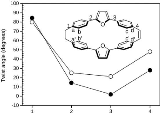
In order to compare the calculated MIM results with the molecular structures in detail, we optimized the lowest excited state geometry of cyclophanene 2*. After photoexcitation, the geometry of cyclophanene 2 will reorganize the nuclei coordinates to a more planar structure. The photo-induced planarity is due to the C-C single bond along the conjugated path that will exchange the length to adapt more double bond characters from reducing antibonding character and increasing the bonding character by the occupied and unoccupied orbitals, respectively. As shown in Figure 1, we can see that the twist angle of the position 4 of the cyclophanene 2* can be reduced from about 50o to lower than 30o. By the photo-induced planarity, we can rationalize by the MIM results, the cyclophanene 2* (sp2) can enhance the CT-exciton from 2.1% to 8.0% (in Table 1) through bond mechanism. In sp3 tether, the CT contribution of cyclophanene 2* (sp3) (0.90%) is slightly large than cyclophanene 2 (sp3) (0.27%). About the factor, we can have a sensible explanation by the critical distances in Figure 1. The sharp decrease (about 20 sp3 tether sp2 tether T-Space:T-Bond
phane 1 16.6347 --- ---
phanene 1 17.3561 17.7454 98%:2%
phane 2 0.7066 --- ---
phanene 2 0.2699 2.1075 13%:87%
degrees) of the twist angles at position 3 and 4 will lead to stronger conjugation character and this feature can reduce the interchromophore distances. From the interchromophore distances in Figure 1, these data demonstrate that the most important critical distance c (2.77 Å) of cyclophanene 2* is reduced by 0.40 Å compare with the distance c of the cyclophanene 2. The critical distance c is close to the shortest interchromophore distance (2.71 Å) in the through-space cyclophanene 1. Therefore, the two inner cofacial p-orbitals of the critical distance c can enhance the CT% in cyclophanene 2* (sp3) apparently.
Figure 1. Critical twist angles for the cyclophanene 2 in the ground state geometry (open circles) and lowest excited-state
geometry (filled circles). Critical distances of ground state: a-a’=2.995, b-b’=3.586, c-c’=3.169, d-d’=3.025, lowest excited state: a-a’=2.993, b-b’=3.397, c-c’=2.769, d-d’=3.058 (in Å).
After a detailed comparison, we consider this truncated MIM approach is a reliable method to determine the delocalization mechanism in cyclophane systems. Compare our theoretical results with experimental data; we can conclude that the interesting shoulder of the cyclophanene 2 in the absorption spectrum5 can be addressed to a through-bond (π-bond) delocalization mechanism chiefly.
In summary, we have applied the “molecule-in-molecule” technique under the four-state approximation to analyze the through-space and through-bond problems in the cyclophane systems successfully. By this truncated Hamiltonian, the model cyclophanene 1 and 2 can be addressed to through-space and through-bond delocalization in the lowest excited state, respectively. This novel approach can be directly applied to not only cyclophane systems but also many bichromophoric systems.
ACKNOWLEDGMENT
The authors thank the National Science Council of ROC for the financial support.
1 2 3 4 -10 0 10 20 30 40 50 60 70 80 90 100 Tw is t an gl e (de g ree s) C-C bond of interest O O 1 2 3 4 a b c d a' b' c' d'
附件二
Vibrational Contributions to Nonlinear Optical
Coefficients
Chia-Chun Chou and Bih-Yaw Jin
Department of Chemistry, National Taiwan University, Taipei, Taiwan
Abstract
Considering a two-level system with a single vibrational mode, we apply the exact sum-over-state (SOS) formulas for the (hyper) polarizabilities expressed in terms of vibronic states to this model. Instead of using Placzek’s approximation, we apply Herzberg-Teller expansion to the sum-over-state formulas including vibrational energy levels. Besides, electrical and mechanical harmonicity are employed. The results we obtain include not only the lattice relaxation expression for vibrational contributions but also the contributions of the next higher order terms. The method we present here is also applied to multi-level and multi-mode system.
I. Introduction
There has been growing interest in the study of nonlinear polarizabilities motivated largely by the potential for using this property in the design of optical communication devices. The design of materials with large optical nonlinearities is an active and well-reviewed area of research [1]. Nonlinear optical processes are governed by molecular hyperpolarizabilities. These properties can be divided into contributions originating from the effects of electric fields on (a) electronic motions and (b) nuclear motions. The past decade has been an interesting number of calculations of vibrational polarizabilities and hyperpolarizabilities [2-4]. On the one hand, polarizabilities and hyperpolarizabilities can be defined by a perturbation theory treatment of the electric fields and this gives rise to sum-over-state formulas in terms of vibronic energies and dipole moment matrix elements. The effect these terms including vibrational levels have on the calculated second hyperolarizability was also examined [3]. On the other hand, a semiclassical treatment is presented by Zerbi and coworkers which allows deriving an explicit analytical expression for this contribution in terms of vibrational spectroscopic observables [2]. The lattice relaxation expression has been obtained from the exact sum-over-state formulas by using Placzek’s approximation [4]. The purpose here is to derive the lattice relaxation expression from the sum-over-state formulas by taking into account the vibrational energies in the denominators of the sum-over-state formulas instead of using Placzek’s approximation.
We begin by considering a two-level system with a single vibrational mode, applying the exact sum-over-state formulas for the (hyper)polarizabilities expressed in terms of vibronic states to this model (Sec. II). The vibrations are described by
displaced, one-dimensional harmonic oscillators. Within the double harmonic
approximation (electrical and mechanical harmonicity), not only the lattice relaxation expression for vibrational contributions but also the contributions of the next higher order terms can be also obtained by using Herzberg-Teller expansion and by making use of a formula developed by Ting [5]. In Sec. III, the method we here employ is applicable to multi-level and multi-mode system. Finally, in Sec. IV, the results are discussed and compared to earlier work.
II. Two level system with a single vibrational mode
In this section, we will consider a two level system with a single vibrational mode. The vibrational levels of the ground and excited electronic states will be modeled by harmonic oscillators (mechanical harmonicity approximation). For simplicity, the oscillators are assumed to have identical frequencies
ω
, but the minima for the ground electronic state and for the excited electronic state are displaced. Thedifference in energy between the minima of the two electronic states will be called ∆.
A. Polarizability
From sum-over-state method, the polarizability
α
can be expressed as∑
≠ − = ′ = 0 0 0 0 ! 2 1 m Em E m mµ
µ
α
α
(2.1) Considering a two level system with a single vibrational mode, the polarizability is∑
∑
= ≠ − + − = ′ 0 0 2 0 0 2 0 0 m em g m gm g E E m e g E E gm gµ
µ
α
(2.2)The bar over the m in the m indicates that this is a vibrational level of the excited
electronic state, m being levels of the ground state. Within the Born-Oppenheimer
approximation, we can write the dipole moment of the ground electronic state as a function of the vibrational coordinate and expand it in a Taylor series about the minimum of the ground electronic state. For simplicity, we set the minimum for the ground electronic state to be zero. Furthermore, the electronic transition moment is only expanded to the first derivative term (electrical harmonicity approximation). Therefore,
( )
Q m gm g0µ
= 0µ
gg (2.3) and( )
( )
Q Q Q gg gg gg 0 0 ∂ ∂ + =µ
µ
µ
(2.4) Substituting the equation (2.3) and (2.4) into the first term in the equation (2.2), we can obtain∑
= ∆+ + ∂ ∂ ∂ ∂ = ′ 0 2 0 0 0 2 1 m gg gg m m e g Q Q k ω µ µ µ α η (2.5) where k is the force constant of the ground vibrational state.The first term in the equation (2.5) is the lattice relaxation expression for vibrational contributions to the polarizability. If the vibrational frequencies are much smaller than the electronic frequencies, i.e. ηω<< ∆, the first term in the equation (2.5) will dominate. Moreover, the first term in the equation (2.5) is a pure vibrational
contribution to the polarizability. That is to say, no electronic excitation is involved. However, the second term in the equation (2.5) is the other type of the contribution to the polarizability. The contribution comes from the coupled motion of the electronic excitation and the nuclear vibration within the adiabatic approximation.
Considering the second term in the equation (2.5), we obtain
∑
∑
= = ∆+ = + ∆ 0 0 2 0 0 0 m eg ge m m m m m m e g ω µ µ ω µ η η (2.6)We will expand the equation (2.6) in powers of ∆ ω η ,
∑
∑
= = − ∆ + ∆ − × ∆ = + ∆ 0 2 2 0 2 1 0 0 1 0 m eg ge m m m m m m m e g Λ η η ηω
ω
µ
µ
ω
µ
(2,7) Since the vibrational levels of the excited state m form a complete set, the firstterm in the equation (2.7) is
∑
=0 0 0 m eg ge m mµ
µ
0 2 0 geµ
= (2.8) We also write the electronic transition moment as a function of the vibrationalcoordinate and expand it in a Taylor series about the minimum of the ground electronic state.
( )
( )
Q Q Q ge ge ge 0 0 ∂ ∂ + =µ
µ
µ
(2.9) Substituting the equation (2.9) into the second term in the equation (2.8), we can obtain( )
ω µ µ µ m Q ge ge ge 2 0 0 0 2 0 2 2 η ∂ ∂ + = (2.10) Similarly, we substitute the equation (2.9) into the second term in the equation (2.7)∑
=0 0 0 m eg ge m m mµ
µ
( )
( )
(
)
∂ ∂ + + ∂ ∂ + =∑
= 0 0 0 0 0 0 0 0 0 0 2 0 0 0 2 Q m m Q Q m m Q Q m m Q m m m ge m ge ge ge µ µ µ µ (2.11)Since the Franck-Condon factor for a two level system with a single vibrational mode is ! 0 2 m e S m I S m − = = (2.12)
the first term in the equation (2.11) can be reduced by S m m m m =
∑
∞ =0 0 0 (2.13) The second term in the equation (2.11) can be simplified by the raising and lowering operator formalism of the harmonic oscillator.
∑
∞(
)
= + 0 0 0 0 0 m m m Q Q m m m∑
∞ = = 0 1 0 2 2 m m m m mω η (2.14)The summations in the equation (2.14) have been given by Ting [5]. Hence, the second term in the equation (2.11) is
(
)
∑
∞ = + 0 0 0 0 0 m m m Q Q m m m − = 2 2 2 δ ω m η (2.15) where δ serves as a dimensionless measure of the displacement d of the oscillators0 0 2 Q d = δ (2.16) In the same way, we can obtain the third term in the equation (2.11)
(
1)
2 1 2 0 0 0 2 0 + = =∑
∑
∞ = ∞ = S m m m m Q m m Q m m m ω ω η η (2.17) Therefore, we obtain∑
=0 0 0 m eg ge m m m µ µ( )
( )
( )
(
1)
2 2 0 0 2 0 0 2 + ∂ ∂ + − ∂ ∂ + = S m Q m Q S ge ge ge ge ω µ δ ω µ µ µ η η (2.18)Through the same process, we can obtain the polarizability to the order of
2 ∆ ω η
( )
( )
( )
(
)
( ) (
)
( )
(
)
(
)
∆ + + + ∂ ∂ + + ∂ ∂ − + ∆ + + ∂ ∂ + − ∂ ∂ + ∆ − ∆ + ∂ ∂ ∆ + ∆ + ∂ ∂ ∂ ∂ = ′ 3 2 2 0 0 2 2 2 0 0 2 2 0 2 0 0 1 5 2 1 2 0 1 0 1 2 ) ( 0 0 1 2 1 0 2 1 ω ω µ µ µ µ ω ω µ µ µ µ ω ω µ µ µ µ α η η η η η η O S S m Q S d Q S S S m Q d Q S m Q Q Q k ge ge ge ge ge ge ge ge ge ge gg ggThe first term is the lattice relaxation expression for vibrational contributions to the polarizability and the second term is the electric contribution to the polarizability. Consequently, if the vibrational frequencies are much smaller than the electronic frequencies (ηω <<∆), we can find that the dominant vibrational contribution to the polarizability
α
is mainly from the pure vibrational motion. Besides, the third term in the equation and the second term, the electric contribution to the polarizability, are the same order.B. First hyperpolarizability
(
)(
)
∑
(
)
∑∑
≠ ≠ ≠ − − − − = ′ = 0 0 2 0 0 0 0 0 0 0 0 0 0 ! 3 1 m m m n m n E E m m E E E E n n m mµ
µ
µ
µ
µ
µ
β
β
(2.19)Considering a two level system with a single vibrational mode, the first hyperpolarizability is
(
)(
)
(
)(
)
(
)(
)
(
)(
)
(
)
∑
(
)
∑
∑∑
∑∑
∑∑
∑∑
= ≠ = = = ≠ ≠ = ≠ ≠ − − − − − − + − − + − − + − − = ′ 0 0 2 2 0 0 2 2 0 0 0 0 0 0 0 0 0 0 0 0 0 0 0 0 0 0 0 0 0 0 0 0 0 0 0 0 0 0 m em g m gm g m n em g en g m n em g gn g m n gm g en g m n gm g gn g E E m e g g g E E gm g g g E E E E g n e n e m e m e g E E E E g gn gn m e m e g E E E E g n e n e gm gm g E E E E g gn gn gm gm g µ µ µ µ µ µ µ µ µ µ µ µ µ µ µ µ β (2.20) Making the same approximation, the pure vibrational terms in the equation (2.20) can be expressed as(
)(
)
∑
(
)
∑∑
≠ ≠ ≠ − 0 2 2 0 0 0 0 0 0 0 m m n m gm g g g n m g gn gn gm gm gω
µ
µ
ω
ω
µ
µ
µ
η η η (2.21)Substituting the equation (2.3) and the equation (2.4) into the equation (2.21), we can find that there is no pure vibrational contribution to the first hyperpolarizability β. Subsequently, the terms that have only one pure vibrational frequency in the denominators are the second term and the third term in the equation (2.20).
(
)(
)
∑∑
(
)(
)
∑∑
= ≠ ≠ = ∆+ + + ∆ 0 0 0 0 0 0 0 0 m n m n m n g gn gn m e m e g n m g n e n e gm gm g ω ω µ µ µ ω ω µ µ µ η η η η (2.22)Substituting the equation (2.3) and the equation (2.4) into the equation (2.22), we can obtain
( )
∑
=(
)
( )
∑
=(
∆+)
∂ ∂ + + ∆ ∂ ∂ 0 0 0 0 1 0 0 1 0 1 1 0 m gg n gg m g m e m e g Q Q n g n e n e g Q Q ω µ µ µ ω ω µ µ µ ω η η η η (2.23) Since the matrix elements in the equation (2.23) are real and the n and m are dummy variables, the equation (2.23) can be written as( )
∑
=(
∆+)
∂ ∂ 0 0 0 1 1 0 2 n gg n g n e n e g Q Q ω µ µ µ ω η η (2.24)Following the similar procedure for the polarizability
α
, the summation in the equation (2.24) is then∑
= − ∆ + ∆ − × ∆ 0 2 2 1 0 1 1 n eg ge n n n n Λ η ηω
ω
µ
µ
(2.25)Using the completeness relationship of the vibrational levels of the excited state n
and the equation (2.9), the first term in the equation (2.25) become
∑
=0 0 1 n eg ge n n µ µ 2( )
0 1 0 0 Q Q ge ge ∂ ∂ = µ µ (2.26) Therefore, the first hyperpolarizability β to the order of0 ∆ ω η turns into
( )
4( )
0 0 1 1 0 1 0 0 Q Q Q Q ge ge gg ∂ ∂ ∂ ∂ ∆ ≅ ′ µ µ µ ω β η (2.27)On the other hand, the electrical contribution to the polarizability
α
is∆ = 2 2 ge e
µ
α
(2.28) The first derivative of the electrical contribution to the polarizabilityα
with respect to the vibrational mode at the minimum of the ground electronic state is( )
∆ ∂ ∂ = ∂ ∂ 0 0 0 4 Q Q ge ge e µ µ α (2.29)Substituting the equation (2.29) into the equation (2.27), we can obtain
0 0 2 1 ∂ ∂ ∂ ∂ ≅ ′ Q Q k e gg α µ β (2.30) where ω m Q Q Q 2 1 0 0 1 1
0 = 2 = η has been used. The k in the equation (2.30)
is the force constant of the ground vibrational state. The equation (2.30) is the lattice relaxation expression for vibrational contributions to the first hyperpolarizability β. Consequently, if the vibrational frequencies are much smaller than the electronic frequencies (ηω <<∆), we can find that the dominant contribution to the first hyperpolarizability β is mainly from the term in the equation (2.30).
Following the similar procedure for the polarizability
α
, we can find the contributions of the next higher order terms to the first hyperpolarizability β. Considering the terms that have ∆2 in the denominators, we have to include thesecond term in the equation (2.25) and the fourth term and the sixth term in the equation (2.20). The fourth term and the sixth term in the equation (2.20) are
(
)(
)
∑
(
)
∑∑
= = = ∆+ − + ∆ + ∆ 0 2 2 0 0 0 0 0 0 0 m m n m m e g g g n m g n e n e m e m e gω
µ
µ
ω
ω
µ
µ
µ
η η η (2.31)We expand the first term in the equation (2.31) in powers of ∆ ω η
[
(
)
− ∆ + − × ∆∑∑
= = Λ ηω µ µ µ m m n n m n m n eg ee ge 0 1 0 1 0 0 2 (2.32)Keeping the equation (2.32) to the order of 12
∆ , we can obtain
∑∑
=0 =0 0 0 m n eg ee ge m m µ n n µ µ( ) ( )
0 0 2( )
0( )
0 0 2 0 2 0 0 0 2 Q Q Q Q ge ee ee ge ge ee ge ∂ ∂ + ∂ ∂ ∂ ∂ + =µ µ µ µ µ µ µ (2.33)Similarly, the second term in the equation (2.31) can be also expanded to the order of
2 1 ∆ . That is to say,
(
)
∑
=0 ∆+ 2 2 0 m m m e gω
µ
η∑
= + ∆ − × ∆ = 0 2 0 0 1 2 3 1 m eg ge m m m Λ ηω µ µ (2.34)Keeping the equation (2.34) to the order of 12 ∆ , we can obtain
∑
=0 0 0 m eg ge m m µ µ( )
0 0 2 0 2 0 2 Q Q ge ge ∂ ∂ + =µ µ (2.35)Hence, the equation (2.31) to the order of 12
∆ turn out to be
( )
( ) ( )
( )
(
( )
( )
)
∂ ∂ − + ∂ ∂ ∂ ∂ ∆ + ∆ − 2 0 0 0 2 2 2 2 2 0 0 0 0 0 0 0 0 Q Q Q Q ge gg ee ee ge ge ge gg ee µ µ µ µ µ µ µ µ µ (2.36) Subsequently, the second term in the equation (2.25) is∑
= ∆ − 0 2 1 0 n eg ge n n n µ µ ω η (2.37) Substituting the equation (2.9) into the equation (2.37), we can obtain( )
( )
(
)
∂ ∂ + + ∂ ∂ +∑
= 0 1 0 1 0 1 0 0 1 0 2 0 0 0 2 Q n n Q Q n n Q Q n n Q n n n ge n ge ge ge µ µ µ µ (2.38)Using the raising and lowering operator formalism of the harmonic oscillator and the summations have been given by Ting [5], we can simplify the equation (2.37). Therefore,
∑
=0 0 1 n eg ge n n n µ µ( )
( )
(
)
− ∂ ∂ + + ∂ ∂ + − =δ
ω
µ
ω
µ
µ
δ
µ
2 3 2 1 2 2 0 2 0 2 0 0 2 m Q S m Q ge ge ge ge η η (2.39) The term of the order of 12∆ in the equation (2.24) is then
( )
( )
( )
(
)
− ∂ ∂ + + ∂ ∂ + − ∆ − ∂ ∂ δ ω µ ω µ µ δ µ ω µ ω 2 3 2 1 2 2 0 2 0 1 0 2 2 0 0 2 2 0 Q m S m Q Q Q ge ge ge ge gg η η η η (2.40) Combining the equation (2.36) with the equation (2.40), we can obtain( )
( ) ( )
( )
(
( )
( )
)
∂ ∂ − + ∂ ∂ ∂ ∂ ∆ + ∆ − 2 0 0 0 2 2 2 2 2 0 0 0 1 0 0 0 Q Q Q m ge gg ee ee ge ge ge gg ee µ µ µ µ µ µ ω µ µ µ η( )
( )
(
)
− ∂ ∂ + + ∂ ∂ + − ∂ ∂ ∆ − δ ω µ ω µ µ δ µ µ ω 2 3 2 1 2 2 0 2 0 2 2 2 0 0 2 0 2 m Q S m Q Q m ge ge ge ge gg η η η (2.41) where ω m Q 2 0 0 2 = η andω
m Q 2 10 = η have been used.
Therefore, combining the equation (2.41) with the equation (2.30), we can write the first hyperpolarizability β as
( )
( ) ( )
0 0 0 2 1 2 2 0 0 ge gg ee e gg Q Q k µ µ µ α µ β ∆ − + ∂ ∂ ∂ ∂ = ′( )
(
( )
( )
)
∂ ∂ − + ∂ ∂ ∂ ∂ ∆ + 2 0 0 0 2 2 2 0 0 0 1 Q Q Q m ge gg ee ee ge ge µ µ µ µ µ µ ω η( )
( )
(
)
− ∂ ∂ + + ∂ ∂ + − ∂ ∂ ∆ − δ ω µ ω µ µ δ µ µ ω 2 3 2 1 2 2 0 2 0 2 2 2 0 0 2 0 2 m Q S m Q Q m ge ge ge ge gg η η η (2.42) The first term in the equation (2.42) is the lattice relaxation expression forvibrational contributions to the first hyperpolarizability. If the vibrational frequencies are much smaller than the electronic frequencies, i.e. ηω <<∆, the first term in the equation (2.42) will dominate. Moreover, there is no pure vibrational contribution to the first hyperpolarizability. That is to say, the contribution of the order of
∆ 1
to the first hyperpolarizability comes from the coupled motion of the electronic excitation and the nuclear vibration within the adiabatic approximation. Besides, the second term in the equation (2.42), the electric contribution to the first hyperpolarizability, and the other terms are the same order.
C. Second hyperolarizability
From sum-over-state method, the second hyperpolarizability γ can be expressed as
(
)(
)(
)
∑
(
)
∑
(
)
∑ ∑∑
≠ ≠ ≠ ≠ ≠ − − − − − − = ′ = 0 0 2 0 0 0 0 0 0 0 0 0 0 0 0 0 0 ! 4 1 m m k k k m n k m n E E m m E E k k E E E E E E n n m m k k µ µ µ µ µ µ µ µ γ γ (2.43) whereµ
=µ
− gµ
g . Following the similar procedure for the firsthyperpolarizability β, we can write the pure vibrational terms in the equation (2.43) as
(
)(
)(
)
(
)
∑
(
)
∑
∑ ∑∑
≠ ≠ ≠ ≠ ≠ − − − − − − 0 0 2 0 0 0 0 0 0 0 0 0 0 0 0 0 0 m gm g k gk g k m n gk g gm g gn g E E g gm gm g E E g gk gk g E E E E E E g gn gn gm gm gk gk g µ µ µ µ µ µ µ µ (2.44)Under the same approximation, we can simplify the equation (2.44). The equation (2.44) then become
( )
( )
2 2 0 2 2 0 3 2 2 4 0 3 0 1 0 1 1 2 1 1 0 2 1 Q Q Q Q Q Q Q gg gg gg ∂ ∂ ∂ ∂ − ∂ ∂ µ µ ω µ ω η η (2.45) Using ω m Q 2 1 0 2 = η and ω m Q2 2 = η1 , we can find that the equation (2.45) is
equal to zero. Like the first hyperpolarizability β, there is also no pure vibrational contribution to the second hyperpolarizability γ .
Next, we consider the terms that have two pure vibrational frequencies in the denominators.
(
)(
)(
)
(
)(
)(
)
(
)(
)(
)
(
)
∑
(
)
∑
∑ ∑∑
∑ ∑∑
∑ ∑∑
≠ = ≠ ≠ = ≠ = ≠ = ≠ ≠ − − − − − − + − − − + − − − 0 0 2 0 0 0 0 0 0 0 0 0 0 0 0 0 0 0 0 0 0 0 0 0 0 0 0 0 0 0 0 0 0 m gm g k ek g k m n gk g gm g en g k m n gk g em g gn g k m n ek g gm g gn g E E g gm gm g E E g k e k e g E E E E E E g n e n e gm gm gk gk g E E E E E E g gn gn m e m e gk gk g E E E E E E g gn gn gm gm k e k e g µ µ µ µ µ µ µ µ µ µ µ µ µ µ µ µ (2.46)The equation (2.46) can be reduced to
( )
(
)
( )
(
)
( )
∑
(
)
∑
∑
= = = + ∆ − + ∆ + + ∆ 0 2 2 0 2 0 2 0 0 1 0 1 1 0 1 1 0 2 0 0 1 1 2 k m k k g k e k e g g g m g m e m e g g g g g k g k e k e g g g g g ω µ µ ω µ ω µ µ ω µ µ ω µ µ ω µ µ η η η η η η (2.47) We expand the summations in the equation (2.47) in terms of∆ ω η .
(
)
∑
∑
= = + ∆ − × ∆ = + ∆ 0 0 1 2 0 1 2 0 k eg ge k k k k k g k e k e g Λ η η ω µ µ ω µ µ (2.48)(
)
∑
∑
= = + ∆ − × ∆ = + ∆ 0 0 1 1 1 1 1 1 m eg ge m m m m m g m e m e g Λ η η ω µ µ ω µ µ (2.49)∑
∑
= = + ∆ − × ∆ = + ∆ 0 0 1 0 0 1 0 0 k eg ge k k k k k g k e k e g Λ η η ω µ µ ω µ µ (2.50) The first terms in the equations (2.48), (2,49) and (2.50) are then∑
=0 2 0 k eg ge k kµ
µ
0 2 2 2 0 Q Q ge ∂ ∂ = µ (2.51)∑
=0 1 1 m eg ge m m µ µ( )
∂ ∂ + = 0 1 2 1 2 0 2 Q Q ge geµ
µ
(2.52)∑
=0 0 0 k eg ge k k µ µ( )
0 0 2 0 2 0 2 Q Q ge ge ∂ ∂ + =µ µ (2.53) Therefore, the equation (2.47) expanded to the order of∆ 1 turns into ∆ ∂ ∂ ∂ ∂ 1 1 2 0 2 0 2 Q Q k ge gg
µ
µ
(2.54) where k is the is the force constant of the ground vibrational state. Consequently, if the vibrational frequencies are much smaller than the electronic frequencies, i.e.∆ <<
ω
Subsequently, considering the terms involved in ∆2 in the denominators, we have
to include not only the second terms in the equations (2.48), (2,49) and (2.50) but also the terms that have only one pure vibrational frequency in the denominators.
Namely,
(
)(
)(
)
(
)(
)(
)
(
)(
)(
)
(
)
∑
(
)
∑
∑ ∑∑
∑ ∑∑
∑ ∑∑
= ≠ = = ≠ = ≠ = ≠ = = − − − − − − + − − − + − − − 0 0 2 0 0 0 0 0 0 0 0 0 0 0 0 0 0 0 0 0 0 0 0 0 0 0 0 0 0 0 0 0 0 m em g k gk g k m n ek g em g gn g k m n ek g gm g en g k m n gk g em g en g E E g m e m e g E E g gk gk g E E E E E E g gn gn m e m e k e k e g E E E E E E g n e n e gm gm k e k e g E E E E E E g n e n e m e m e gk gk g µ µ µ µ µ µ µ µ µ µ µ µ µ µ µ µ (2.55)At first, we can simplify the equation (2.55).
(
)(
)
(
)
(
)(
)
( )
∑
(
)
∑∑∑
∑∑
= = ≠ = = = + ∆ − + ∆ + ∆ + + ∆ + ∆ 0 2 0 0 0 0 0 0 0 0 1 1 0 0 0 0 1 1 0 2 m k m n m n m g m e m e g g g g g n m k g n e n e gm gm k e k e g n m g n e n e m e m e g g g ω µ µ ω µ µ ω ω ω µ µ µ µ ω ω µ µ µ ω µ η η η η η η η η (2.56)In the same way, the summations in the equation (2.56) are expanded in terms of ∆
ω
η and we keep the summations to the order of 12
∆ .
(
)(
)
∑∑
∑∑
= = = = ∆ ≅ + ∆ + ∆ 2 0 0 0 0 0 1 1 0 1 m n m n g n e n e m e m e g n m g n e n e m e m e g µ µ µ ω ω µ µ µ η η(
)
(
)(
)
∑ ∑∑
=0 ≠0 =0 ∆+ ∆+ 0 0 k m n k m n g n e n e gm gm k e k e g ω ω ω µ µ µ µ η η η(
)
∑∑∑
= ≠ = ∆ ≅ 0 0 0 2 0 0 1 k m n m g n e n e gm gm k e k e g ω µ µ µ µ η(
)
∑
∑
= = ∆ ≅ + ∆ 2 0 0 2 0 0 1 0 0 m m g m e m e g m g m e m e g µ µ ω µ µ η (2.57) Through the similar procedures for the polarizabilityα
and the first(
)(
)
(
)
(
)(
)
( )
∑
(
)
∑∑∑
∑∑
= = ≠ = = = + ∆ ∂ ∂ − + ∆ + ∆ + + ∆ + ∆ ∂ ∂ 0 2 2 0 2 0 0 0 0 0 0 0 0 1 0 0 0 0 1 1 0 2 m gg k m n m n gg m g m e m e g Q Q n m k g n e n e gm gm k e k e g n m g n e n e m e m e g Q Q ω µ µ µ ω ω ω ω µ µ µ µ ω ω µ µ µ µ ω η η η η η η η η( )
( )
[
]
( )
( )
( )
2 2 1 0 2 1 2 3 1 0 1 0 0 0 2 1 1 4 0 2 2 0 2 2 0 0 2 0 0 0 2 0 0 2 ω µ µ µ ω µ µ µ µ µ µ µ µ µ µ µ η η ∂ ∂ + ∂ ∂ + ∂ ∂ ∂ ∂ ∂ ∂ + ∂ ∂ ∂ ∂ + ∂ ∂ ∂ ∂ − × ∆ = Q k Q k k Q Q Q Q Q k Q Q k ge ge ge gg ee ge gg ee ge gg ge ge gg ee( )
∂ ∂ ∂ ∂ + ∂ ∂ − 2 2 1 0 2 1 2 0 2 0 2 2 0 2 µ µ µ ω µ η Q Q k Q k gg ge gg ge (2.58)where k is the is the force constant of the ground vibrational state.
Furthermore, we have to include the second terms in the equations (2.48), (2,49) and (2.50). Using the raising and lowering operator formalism of the harmonic oscillator and the summations have been given by Ting [5], we can simplify the second terms in the equations (2.48), (2,49) and (2.50). Therefore, the terms in the equation (2.47) of the order of 12
∆ then turn out to be
( )
( )
(
)
+ ∂ ∂ + ∂ ∂ − × ∂ ∂ ∆ − 4 5 2 4 2 0 0 2 1 1 2 0 0 2 2 0 2 S m Q m Q k Q ge ge ge ge gg ω µ δ ω µ µ µ µ η η (2.59)Collecting all the terms of the order of 12
∆ , the terms in the equations (2.58) and (2.59), we can obtain
( )
( )
[
]
( )
( )
( )
( )
( )
(
4 5)
2 2 1 1 4 2 0 2 1 1 2 3 1 1 2 2 1 1 2 2 1 1 0 1 1 0 2 1 1 0 1 1 0 0 0 2 1 1 2 0 2 0 2 2 0 2 0 2 2 0 0 2 0 2 4 0 2 2 2 0 2 0 2 2 2 0 2 2 2 0 2 2 0 0 2 2 0 0 2 + ∂ ∂ ∂ ∂ ∆ − ∂ ∂ ∂ ∂ ∆ + ∂ ∂ ∂ ∂ ∂ ∂ ∆ + ∂ ∂ ∆ + ∂ ∂ ∂ ∂ ∆ + ∂ ∂ ∆ − ∂ ∂ ∆ + ∂ ∂ ∂ ∂ ∆ + ∂ ∂ ∂ ∂ − ∆ S Q Q k m Q Q k k Q Q Q Q k Q Q k Q k Q k Q Q k Q Q k ge gg ge ge gg gg ee ge ge gg ge gg ge ge ge gg ee ge gg ge ge gg ee ω µ µ δ ω µ µ µ ω µ µ µ ω µ ω µ µ µ µ µ µ µ µ µ µ µ µ µ µ η η η η η (2.60) Simplifying the equation (2.60), we can obtain( )
( )
[
]
( )
( )
( )
( )
(
)
( )
δ ω µ µ µ ω µ µ µ ω µ ω µ µ µ µ µ µ µ µ µ µ µ µ µ µ 4 2 0 2 1 1 2 3 1 1 2 2 1 1 1 2 2 1 0 1 1 0 2 1 1 0 1 1 0 0 0 2 1 1 0 2 0 2 2 0 0 2 0 2 4 0 2 2 2 0 2 0 2 2 2 0 2 2 2 0 2 2 0 0 2 2 0 0 2 m Q Q k k Q Q Q Q k S Q Q k Q k Q k Q Q k Q Q k ge ge gg gg ee ge ge ge gg gg ge ge ge gg ee ge gg ge ge gg ee η η η η ∂ ∂ ∂ ∂ ∆ + ∂ ∂ ∂ ∂ ∂ ∂ ∆ + ∂ ∂ ∆ + + ∂ ∂ ∂ ∂ ∆ − ∂ ∂ ∆ − ∂ ∂ ∆ + ∂ ∂ ∂ ∂ ∆ + ∂ ∂ ∂ ∂ − ∆ (2.61) On the other hand, the electrical contribution to the first hyperpolarizability β is(
)
2 2 6 ∆ − = ge gg ee eµ
µ
µ
β
(2.62) The first derivative of the electrical contribution to the first hyperpolarizability β with respect to the vibrational mode at the minimum of the ground electronic state is( )
(
( )
( )
)
( )
∆ ∂ ∂ − + ∆ ∂ ∂ − ∂ ∂ = ∂ ∂ 0 2 2 0 0 0 0 2 0 0 6 0 6 Q Q Q Q ge ge gg ee ge gg ee eµ
µ
µ
µ
µ
µ
µ
β
(2.63)Through the equation (2.63) and the equation (2.29), the first four terms in the equation (2.61) can be written as
∂ ∂ ∂ ∂ + ∂ ∂ ∂ ∂ 0 0 0 0 6 1 8 1 1 Q Q Q Q k e gg e e α µ β α (2.64)
Hence, the terms involved in ∆2 in the denominators then become
(
)
( )
δ ω µ µ µ ω µ µ µ ω µ ω µ µ β µ α α 4 2 0 2 1 1 2 3 1 1 2 2 1 1 1 2 2 1 6 1 8 1 1 0 2 0 2 2 0 0 2 0 2 4 0 2 2 2 0 2 0 2 2 0 0 0 0 m Q Q k k Q Q Q Q k S Q Q k Q Q Q Q k ge ge gg gg ee ge ge ge gg e gg e e η η η η ∂ ∂ ∂ ∂ ∆ + ∂ ∂ ∂ ∂ ∂ ∂ ∆ + ∂ ∂ ∆ + + ∂ ∂ ∂ ∂ ∆ − ∂ ∂ ∂ ∂ + ∂ ∂ ∂ ∂ (2.65)Combining the equation (2.54) with the equation (2.65), we can write the second hyperpolarizability γ as ∂ ∂ ∂ ∂ + ∂ ∂ ∂ ∂ + ∂ ∂ ∂ ∂ ∆ = ′ 0 0 0 0 2 0 2 0 2 6 1 8 1 1 1 1 Q Q Q Q k Q Q k e gg e e ge gg µ α α µ β µ γ
(
)
( )
δ ω µ µ µ ω µ µ µ ω µ ω µ µ 4 2 0 2 1 1 2 3 1 1 2 2 1 1 1 2 2 1 0 2 0 2 2 0 0 2 0 2 4 0 2 2 2 0 2 0 2 2 m Q Q k k Q Q Q Q k S Q Q k ge ge gg gg ee ge ge ge gg η η η η ∂ ∂ ∂ ∂ ∆ + ∂ ∂ ∂ ∂ ∂ ∂ ∆ + ∂ ∂ ∆ + + ∂ ∂ ∂ ∂ ∆ − (2.66)If the vibrational frequencies are much smaller than the electronic frequencies, i.e. ∆
<<
ω
η , the first term in the equation (2.66) will dominate. The second and the third terms in the equation (2.66) involved in the derivatives of the electrical contribution to the polarizability and of the electrical contribution to the first hyperpolarizability are the lattice relaxation expression for vibrational contributions to the second
hyperpolarizability. Moreover, there is no pure vibrational contribution to the second hyperpolarizability. That is to say, the contribution of the order of
∆ 1
to the second hyperpolarizability comes from the coupled motion of the electronic excitation and the nuclear vibration within the adiabatic approximation. Besides, the other terms in the equation (2.66) and the lattice relaxation expression for vibrational contributions to the second hyperpolarizability are the same order.
III. Multi-level system with multiple vibrational modes
The method in section II is also applicable to multi-level system with multiple vibrational modes. In the same way, the vibrational levels of the ground and excited electronic states will be modeled by harmonic oscillators (mechanical harmonicity approximation). Furthermore, for simplicity, the oscillators of the same mode are assumed to have identical frequencies
ω
, but the minima for the ground electronic state and for the excited electronic state of the same mode are displaced.A. Polarizability
From sum-over-state method, the polarizability
α
can be expressed as∑
≠ − = ′ = 0 0 0 0 ! 2 1 m Em E m m µ µ α α (3.1) Therefore, the electrical contribution to the polaizability turns into∑
∑
∞ = ≠ ∆ = − = ′ 1 2 0 0 i i ge i i i i i E E g e e gµ
µ
µ
α
(3.2)where ∆i = Ei −E0. E and 0 E refer to the ground and the i-th excited electronic i
state energy respectively. If we include multiple vibrational modes with multi-level electronic states, we have
{ }
∑ ∑
∑ ∑
{ }
∑
∞ = = ≠ ∆ + + = ′ 1 0 2 0 0 0 2 0 0 0 0 i m a a i a i i a i i m a a a a a i a m m e g m gm gω
µ
ω
µ
α
η η (3.3) In the equation (3.3),{ }
am0 refers to
(
mo1,mo2,mo3,Λ)
and m denotes the vibrational 10quantum number of the first mode in the ground electronic state, 2 0
m denotes the
vibrational quantum number of the second mode in the ground electronic state and so on. Similarly,
{ }
ai
m refers to
(
mi1,mi2,mi3,Λ)
and1
i
m denotes the vibrational
quantum number of the first mode in the i-th electronic state, 2
i
m denotes the
vibrational quantum number of the second mode in the i-th electronic state and so on. Within the Born-Oppenheimer approximation,
( )
a gg a m Q gm g0µ 0 = 0 µ 0 (3.4)For a collection of oscillators, we have =
∏
( )
a a g0a Q 0 χ and =
∏
( )
a a gm a Q m0 χ awhere χgma denotes the harmonic oscillator eigenfunction of the a-th mode with
vibrational quantum number a
m in the ground electronic state. In the same way, we
can write the dipole moment of the ground electronic state as a function of the vibrational coordinate and expand it in a Taylor series about the minimum of the ground electronic state. For simplicity, we set the minimum for the ground electronic state to be zero. Furthermore, the electronic transition moment is only expanded to the first derivative term (electrical harmonicity approximation). Therefore,
( )
( )
∑
∂ ∂ + = b b b gg gg gg Q Q Q 0 0 µ µ µ (3.5)Substituting the equation (3.5) into the equation (3.4), we obtain
( )
a b b b gg a gg a gg Q m Q m m 0 0 0 0 0 0 0 0∑
∂ ∂ + =µ µ µ (3.6) Since{ }
0a ≠(
0,0,0,Λ)
m for the first summation in the equation (3.3), 0 m0a =0.
0
0 0a =
b m
Q unless a=b, m0a =1a0 and the vibrational quantum numbers of other
modes are equal to zero. Consequently,
a a a gg a gg Q Q 0 0 0 0 1 1 0 ∂ ∂ = µ µ (3.7) where a a a a Q 0 0 2 1 0
ω
µ
η= . Therefore, the first term in the equation (3.3) then becomes
∑
∂∂ a a a a gg a Q Q 2 0 2 0 0 1 0 1µ
ω
η (3.8)By neglecting the second term in the equation (3.3) that has ∆i in the denominator,