創新建材在圓錐量熱儀、表面測試爐及單材耐燃測試儀之火災試驗數據相關性之研究

(1)

國立交通大學

機械工程學系

碩士論文

創新建材在圓錐量熱儀、表面測試爐及

單材耐燃測試儀之火災試驗數據相關性

之研究

The Research for Testing Data Correlation

of New and Innovative Building Materials

between the Cone Calorimeter, the Surface

and SBI Tests

研究生：戴嘉鴻

指導教授：陳俊勳教授

(2)

創新建材在圓錐量熱儀、表面測試爐及單材耐燃測試儀之火災試驗數據相關性之研究

The Research for Testing Data Correlation of New and Innovative Building Materials between the Cone Calorimeter, the Surface and SBI

Tests 研究生：戴嘉鴻 Student：Jia-Hong Dai 指導教授：陳俊勳 Advisor：Chiun-Hsun Chen 國立交通大學機械工程學系碩士論文 A Thesis

Submitted to Department of Mechanical Engineering College of Engineering

National Chiao Tung University In Partial Fulfiillment of the Requirements

For the Degree of Master of Science In Mechanical Engineering

June 2006

Hsinchu, Taiwan, Republic of China

(3)

創新建材在圓錐量熱儀、表面測試爐及單材耐燃測試儀之火災試驗數據相關性之研究學生：戴嘉鴻指導教授：陳俊勳國立交通大學機械工程學系

摘要

本論文以十五種材料分別於圓錐量測儀以及表面測試爐上進行測試，其中圓錐量測儀測試結果依照日本現行防火材料等級分類標準進行分級，而表面測試爐測試結果則依照CNS 6532 進行分級。在圓錐量測儀測試中，也同時探討樣品在水平測試與垂直測試結果的差異性，兩者比較發現在引燃時間和熱釋放率是有所差異，其中水平測試的引燃時間較垂直測試的短，且水平測試的平均180 秒熱釋放率值以及總熱釋放率皆高於垂直測試，因此使用圓錐量熱儀水平測試之數據來分級是較為嚴苛的。另外亦從前述十五種測試材料中挑選其中的七種材料來進行單材耐燃測試儀(SBI) 測試，並依歐盟標準進行分級，另外並與圓錐量測儀以及表面測試爐之分級結果進行比對。結果發現歐盟在建築材料防火等級分類上並沒有材料破裂之限制，且歐盟與日本之防火等級分類中也沒有針對煙產生量作評量，這是他們與 CNS 6532 防火等級性能評估上之主要差異。在相關性分析中，由圓錐量測儀水平與垂直測試實驗中所得到的熱釋放率計算出的火災成長率進行相關性比對，發現圓錐量測儀在水平測試之數據與單材耐燃測試儀相關性較高；表面測試爐與單材耐燃測試儀之發熱性與發煙性相關係數均良好；表面測試與圓錐量測儀在水平與垂直測試之發熱性相關係數均良好；另外表面測試引燃時間與圓錐量測儀在垂直測試之引燃時間相關性良好。

(4)

The Research for Testing Data Correlation of New and Innovative Building Materials between the Cone Calorimeter, the Surface and SBI

Tests

Student: Jia-Hong Dai Advisor: Prof. Chiun-Hsun Chen Department of Mechanical Engineering

National Chiao Tung University

Abstract

Fifteen building materials were selected and tested in the Cone Calorimeter and the surface test, respectively, and they were classified by Japanese classification and CNS 6532 accordingly. Tests in the Cone Calorimeter were performed in the horizontal and vertical directions, respectively, under a fixed incident heat flux 50kW/m2. The results from these two orientations show some differences existed in HRR and ignition time. For the flammable material, the measured average values of HRRav_180s, and THR in the horizontal orientation are higher than those in

vertical one. The ignition time in horizontal orientation is found shorter. Those indicate that the classification using Cone Calorimeter test in horizontal orientation is stringent. In addition, 7 materials from the previously mentioned 15 ones are selected to test in SBI and classified by EU classification. Correlation based on test results of these materials by using these three different standards are given and discussed. It is found that the smoke generation rate and crack appearance are not included in the performance evaluations in Japanese and EU classifications that causes the different ranks in different test methods. The obtained results

(5)

in SBI test are compared with the simulated FIGRA from Cone data. It is found that the correlation between SBI and cone calorimeter test in horizontal orientation is better than the corresponding one with the cone calorimeter test in vertical orientation. The correlation between tdθ value of surface test and THR600s of SBI test finds that the value of R2 is 0.75.

Correlation between the CA value of surface test and maximum 60s mean

value of SPR of SBI test gives the value of R2 is 0.92, indicating that the correlation between the surface and SBI tests are relatively well.From the comparison between HRRav_180s of Cone Calorimeter test in vertical

orientation and tdθ value of the surface test, R2 for the correlation is 0.95. The correlated R2 value between Cone Calorimeter test in horizontal orientation and the surface test is 0.96. Apparently, the correlation between the Cone Calorimeter and the surface tests is relatively well. The correlation for ignition time between cone calorimeter test in vertical direction and the one in surface test is relatively well as well.

(6)

誌謝

兩年碩士時光即將過去，回首其中包含了數不清的歡笑與辛勞、站在實驗室外的窗口無數次以及每天一杯黑咖啡等的珍貴回憶! 感謝恩師陳俊勳教授諄諄教誨，對於研究方法與態度、思考與做事觀念等之啟迪，另外在待人處世亦是或益良多，謹在此向老師致上無比的敬意和感謝。感謝中台技術學院徐一量教授與台灣警察專科學校邱晨瑋教授於口試期間的耐心教導與指正，使得本論文更臻完善。在燃燒防火實驗室的兩年碩士生涯裡，體會到各式各樣的研究生活。感謝宋文義學長這兩年在實驗和論文上的幫忙。感謝大達、文奎、文耀以及小季學長幫忙解答諸多研究上的困惑。同學國華、靜慈、關恕有福同享，有難同當。以及學弟耀文、炳坤以及建宏在忙碌之虞所給予的幫忙，能在燃燒防火實驗室所一起生活的兩年將是我最美好的回憶。另外也感謝隔壁實驗室的純情堡、高個兒以及阿肥，在我最需要幫助時鼓勵我。另外在工研院打工的一年多中，感謝洪大姐、瓊瑤、玟雅以及文濱對於實驗上以及論文上的指導與鼓勵，這一年多來學到很多東西。另外感謝小綠在我寫論文以及準備口試期間的鼓勵。最後要感謝我親愛的父母和老姐，感謝你們長久的支持與關懷。在求學的各階段不斷的給予我鼓勵，你們的支持是我前進最大的力量。最後，僅以此論文獻給我摯愛的家人，謝謝你們。

(7)

LIST OF TABLES

Table 1.1: The apparatus and criteria of classification...4

Table 2.1: Heats of combustion and heats of combustion per gram of oxygen consumed for typical organic liquids and gases ...70

Table 2.2: Heats of combustion and heats of combustion per gram of oxygen consumed for typical synthetic polymers ...70

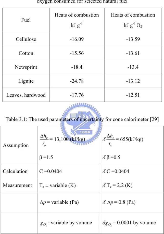
Table 2.3: Heats of combustion and heats of combustion per gram of oxygen consumed for selected natural fuel ...71

Table 3.1: The used parameters of uncertainty for cone calorimeter [29] ...71

Table 3.2: The exhaust temperature of standard for CNS 6532 [6] ...72

Table 3.3: Uncertainties in volume flow measurement in the SBI test [30] ...72

Table 3.4: HRR uncertainty of SBI at the 35 kW level [30] ...73

Table 3.5: HRR uncertainty of SBI at the 50 kW level [30] ...74

Table 3.6: Summary of uncertainty for different levels of SPR [30] ...74

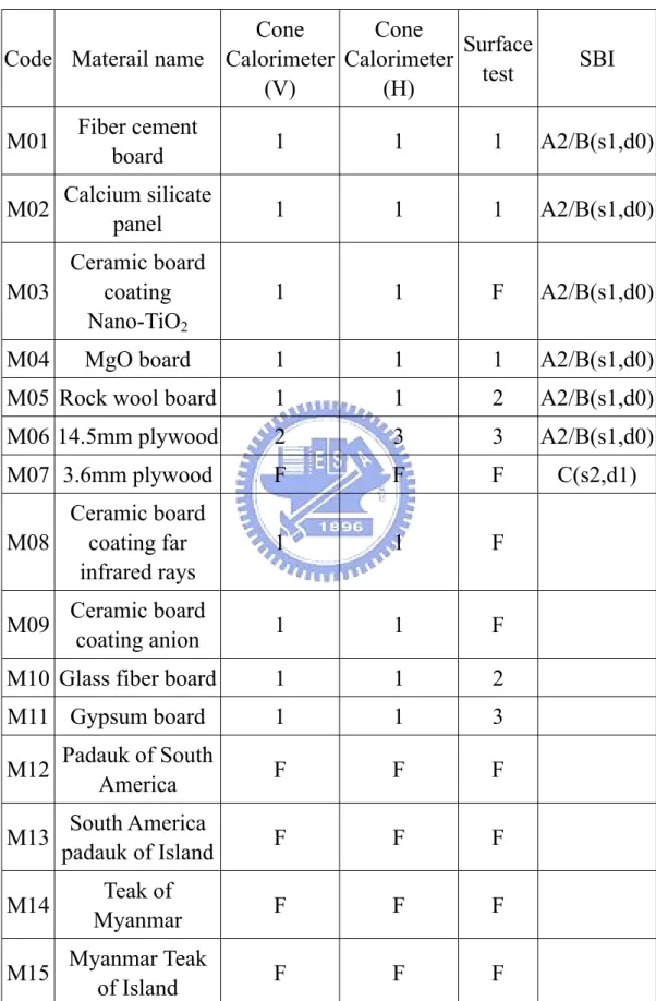
Table 4.1: List of New and Innovative building materials...75

Table 4.2: Major compositions of materials...76

Table 4.3: The classification of Japanese cone calorimeter test...77

Table 4.4: Results of cone calorimeter tested in vertical orientation (average value) ...78

Table 4.5: Results of cone calorimeter tested in horizontal orientation (average value) ...79

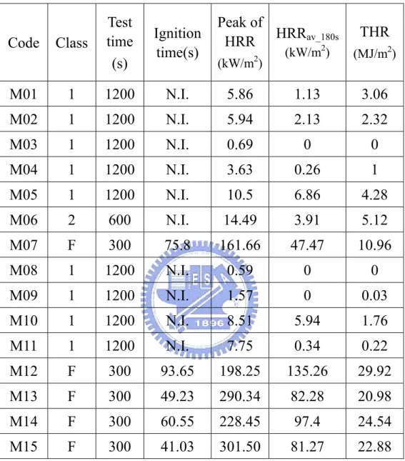
Table 4.6: Classification according to CNS 6532...80

Table 4.7: Results of surface test (average value) ...81

Table 4.8: Results of elementary material test (average value)...82

(13)

Table 4.10: EU classes for construction products excluding flooring ...83

Table 4.11: The summary results of SBI test (average value) ...84

Table 4.12: The classification of SBI test...84

Table 4.13: The classification of Cone Calorimeter, the surface and ...85

SBI tests...85

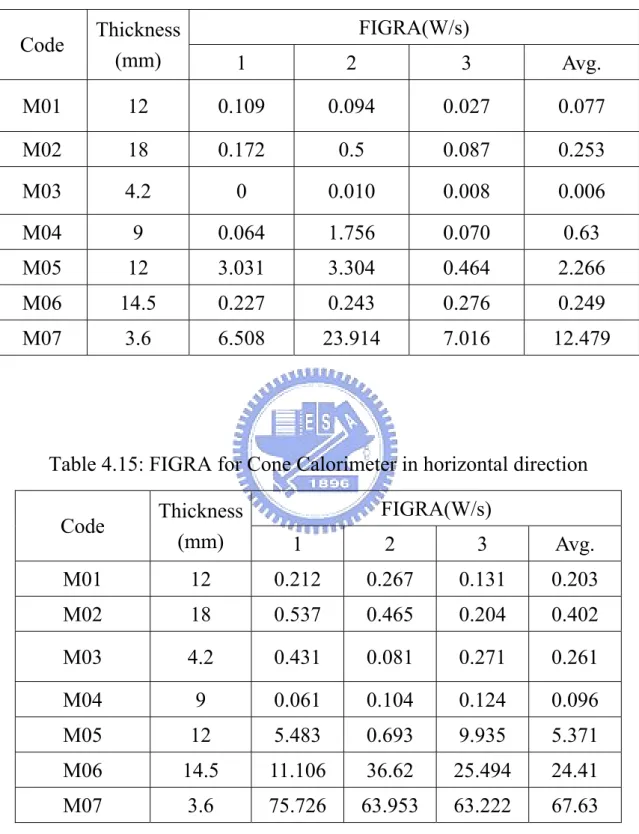
Table 4.14: FIGRA for Cone Calorimeter in vertical direction ...86

(14)

LIST OF FIGURES

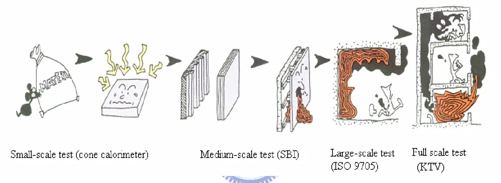
Figure 1.1: The Evolution of Fire Testing Methods ...87

Figure 2.1: The picture of Cone Calorimeter (Cone2) ...88

Figure 2.2: The schematic configuration of the Cone Calorimeter ...88

Figure 2.3: Cone heater (Cone2) ...89

Figure 2.4: Horizontal orientation (Cone2) ...89

Figure 2.5: Vertical orientation (Cone2)...90

Figure 2.6: Gas analyzer instrumentation (Cone2)...90

Figure 2.7: The surface test apparatus ...91

Figure 2.8: The furnace of surface test ...91

Figure 2.9: The average heat flux value of surface test [14] ...92

Figure 2.10: The smoke accumulation box ...92

Figure 2.11: Optical density-measuring system of surface test...93

Figure 2.12: Results and specification of surface test ...93

Figure 2.13: An elementary material test apparatus ...94

Figure 2.14: SBI test ...94

Figure 2.15: Schematic picture of SBI ...95

Figure 2.16: Trolley of SBI...95

Figure 2.17: Gas Control Box and Gas Analysis Rack of SBI...96

Figure 2.18: Exhaust hood and Ring of SBI...96

Figure 2.19: Exhaust system of SBI ...97

Figure 3.1: HRR ± absolute uncertainty and relative uncertainty histories form cone calorimeter results [29] ...97

Figure 3.2: Component uncertainty histories from cone calorimeter results [29] ...98

Figure 4.1: Correlation between vertical and horizontal directions of cone calorimeter tests using HRRav_180s...99

(15)

Figure 4.2: The correlation between FIGRA of cone calorimeter in

vertical direction and SBI tests...100 Figure 4.3: The correlation between FIGRA of cone calorimeter in

horizontal direction and SBI tests...101 Figure 4.4: The correlation between THR600s of SBI test and tdθ of

surface test ...102 Figure 4.5: The correlation between the maximum SPRav_60s of SBI test

and CA value of surface test...103

Figure 4.6: The correlation between 180s mean value of Cone

Calorimeter test in vertical direction and tdθ value of surface test...104 Figure 4.7: The correlation between 180s mean value of Cone

Calorimeter test in horizontal direction and tdθ value of surface test...105 Figure 4.8: The correlation between 180s mean value of Cone

Calorimeter test in vertical direction and tdθ value of surface test without M12...106 Figure 4.9: The correlation between 180s mean value of Cone

Calorimeter test in horizontal direction and tdθ value of surface test without M12 ...107 Figure 4.10: The correlation between ignition time of cone calorimeter in vertical direction and tc value of surface test ...108

Figure 4.11: The correlation between ignition time of cone calorimeter in vertical direction and tc value of surface test without M06 ...109

Figure 4.12: The correlation between ignition time of cone calorimeter in horizontal direction and tc value of surface test ...110

Figure 4.13: The correlation between ignition time of cone calorimeter in horizontal direction and tc value of surface test without M06 ...111

(16)

Appendix

Appendix A...112 Appendix B1...113 Appendix B2...115 Appendix C1...117 Appendix C2...120 Appendix D1...121 Appendix D2...122

Nomenclature

Cone Calorimeter

(17)

As Initially exposed surface area of the specimen m2 C Calibration constant for oxygen consumption

analysis (m·kg·K)

1/2

c

h

Δ Net heat of combustion kJ/g

eff c h _,

Δ _{Effective net heat of combustion} _kJ/g

0

I Initial laser intensity

I Laser intensity measured

K Extinction Coefficient 1/m

m Mass of the specimen kg

mf Mass of the specimen at the end of the test kg mi Mass of the specimen at sustained flaming kg

m& Mass loss rate of the specimen kg/s

e

m& Mass flow rate in exhaust duct kg/s

p

Δ Orifice meter pressure differential Pa

q& _{Heat release rate} _kW

q ′′& Heat release rate per unit area kW/m2

max

q ′′& Maximum value of the heat release rate kW/m2

180

q ′′& The average heat release rate over the period starting

at tig and ending 180s later

kW/m2

300

q ′′& The average heat release rate over the period starting

at tig and ending 300s later kW/m

2

total

q ′′& The total heat released during the entire test MJ/m2 rO Stoichiometric oxygen/fuel mass ratio

t Time s

td Delay time of the oxygen analyser s

tig Time to ignition (sustained flaming) s

t

Δ Sampling time intervals s

Te Absolute temperature of gas at the orifice meter K

(18)

2

O

χ

_{Oxygen analyzer reading, mole fraction of oxygen}

0

2

O

χ

Initial value of oxygen analyzer reading

1

2

O

χ

Oxygen analyzer reading, before delay time

correction f

σ

_{Specific extinction area} _m2_/kg

Surface test

CA Smoke-generation coefficient

tdΘ the area under the test and the standard temperature

curves °C·min

t1 time of sustained flaming after completion of the test sec

Ck cracking of the back surface

SBI

A Area of the exhaust duct at the general

measurement section m

2

c

(

2T₀ / ρ₀

)

0.5 = 22.4 K0.5⋅m1.5⋅kg−0.5

E Heat release per unit volume of oxygen consumed at 298 K, 17200kJ/m3

FIGRA Fire growth rate index W/s

H Relative humidity %

( )

t

HRR_total Total heat release rate of the specimen

and burner kW

burner av

(19)

HRR(t) Heat release of the specimen kW HRRav(t) Average heat release rate of the

specimen kW

I(t) Signal from the light receiver % t

k Flow profile factor

ρ

k Reynolds number correction for the _{bidirectional probe, taken as 1.08} L Length or diameter of the light path

through the exhaust duct m

max.[a(t)] Maximum of a(t) within the given time period

max.[a,b] Maximum of the two values a and b

( )

t p

Δ Pressure difference Pa

p Ambient pressure Pa

SPRtotal(t)

Total smoke production rate of specimen

and burner m

2_/s

SPRav(t) Average of SPR(t) m2/s

SMOGRA Smoke growth rate index m2/s2 SPR(t) Smoke production rate of the specimen m2/s SPRav_burner

The average smoke production rate of

the burner,0± 0.1m2/s m

2_/s

( )

t

T_ms Temperature in general measurement

section K

THR(t) Total heat release of the specimen MJ

THR600s

total heat release of specimen in the first 600s of the exposure period

(

300s≤t≤900s

)

MJ

TSP(ta)

Total smoke production of the specimen within 300s≤t≤ta

m2

( )

t

V Volume flow in the exhaust duct m3/s V298(t) Volume flow of exhaust system, _{normalized at 298K} m3/s

( )

t

(20)

( )

t

xCO₂ Carbon dioxide concentration in mole fraction

2

_ O

a

x Ambient mole fraction of oxygen including water vapor

( )

t

φ

Calculation of the oxygen depletion

(21)

Chapter One

INTRODUCTION

1.1 Motivation

Mankind can feel different aspects of fire. It can provide beneficial ways of living, such as heating source for cooking, warming people and a source of energy for many mechanical devices. On the other hand, fire implies another kind of severe hazard to human being. As a room catches fire, it generates heat, and even toxic and corrosive substances that cause fatal and properties loss. Thus it initiates many scientists and engineers to work together for obtaining a systematic solution to alleviate the loss. Hence many fire testing methods and models have been developed for assessing the fire hazard. The evolution can be seen in Fig. 1.1.

In the very early days, the testing method basically was only used to evaluate the fire performance of material in a bench scale under an assigned environment. These bench scale tests usually were only provided result of pass or fail without any detailed information. However, they served as the baseline for the fire safety regulation. As the advance of material science and technology, many new materials are developed and the above-mentioned test method may not get along with the progress of technologies as expected. Therefore, a revolution testing methodology, termed as reaction-to-fire, was developed in the era of 1990. The Cone Calorimeter (ISO 5660) [1] was the representative testing apparatus. The reaction-to-fire properties of building materials include the flammability, combustibility, toxicity, heat release rate…etc. Among

(22)

them, heat release rate is an important parameter to characterize a fire. It describes the total energy release of a material, or upholstery furniture, or a confined space during burning. As pointed out by Thornton [2] and then Huggett [3], there exists a more or less an approximate constant of heat release per unit mass of oxygen consumed for a large number of organic matters. This constant is given as 13.1MJ/kg of O2. Therefore heat release

rate can be measured by using Oxygen Depletion Method (or Oxygen Consumption Method), which is a well-known method and widely adopted for both bench-scale and large-scale experiments in many fire laboratories all over the world.

The general goal of fire safety regulations is to provide life safety and sufficient property protection in case of fire. In order to achieve this goal, combustibility of materials, fire protection of structures, evacuation arrangements, and relative locations of buildings are set to define how buildings should be designed and constructed for their respective use. Traditionally, fire testing and classification systems are developed individually in different countries, each with its different background and circumstances. A wide variety of requirements has thus been drawn up. However, as a result of the development of transportation facilities and international trade, the harmonization of standards and fire classification systems has become an issue of increasing importance. Canada adopted the cone calorimeter (ASTM 1354) [4] to make classification for the fire performance of building materials in 1992. In the Building Standard Law (BSL) of Japanese, it has already adopted the heat release rate obtained from the cone calorimeter (ISO 5660) [1] as the test criteria to replace the

(23)

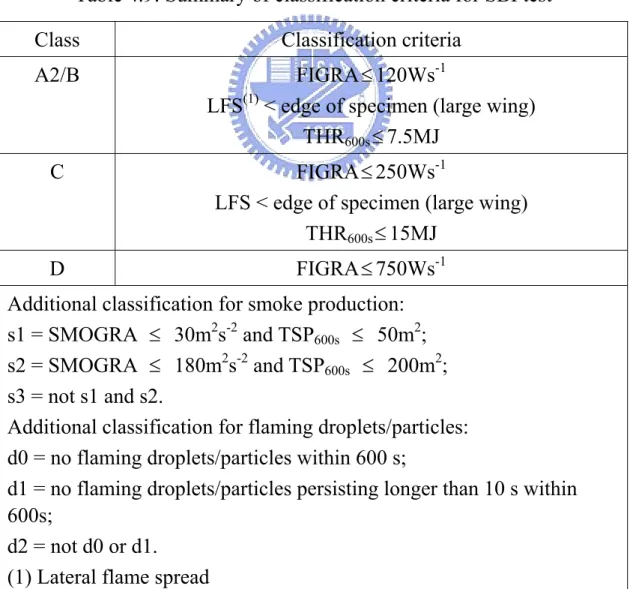
original JIS A 1321 [5], equivalent to Taiwan CNS 6532 [6]; Method of Test for Incombustibility of Interior Finish Material of Buildings. In the European Union (EU), the development of the Euroclass system, EN 13823 [7], was completed in 2002. It defines the fire performance classification of building productions and building components by using the single burning item (SBI) test.

Since 1990s, EU planed to adopt the cone calorimeter test (ISO 5660) [1] for the small-scale test and the room corner test (ISO 9705) [8] for large-scale one. However, it was difficult to obtain the satisfactory correlation between the test results obtained from cone calorimeter and room corner tests respectively, after several years of research. Of course, the room corner test could show the real reaction-to-fire behaviors of materials in a fire, but it cost a lot of time and resource. On the other hand, the small scale fire test of cone calorimeter cannot exhibit the reaction-to-fire properties in the situation of a real fire. Therefore the EU developed a medium-scale test, called single burning item test (EN 13823 [7]), to make a compromise. It was carried out since 2002, and now the building materials, which are intended to be sold in EU, must comply with the proper standard of the SBI test except the fire door of buildings. In addition, for harmonization of fire standards for trains the EU wanted to develop a standard, called prEN 45545-2 [9], to replace all national corresponding standards. According to prEN 45545-2 [9], the burning behaviors of passenger seats for railway vehicles should be tested by including the complete passenger seat, upholstery and head rest, seat shell and arm rest. Test methods consists of ISO 9705(Furniture Calorimeter)

(24)

[8], ISO 5660 (Cone Calorimeter) [1] and ISO 5659-2(Smoke chamber with FTIR) [10]. The FTIR (Fourier Transformation InfraRed spectroscopy) is used for analyzing toxic components. However, this proposed standard is not perfect enough to carry out yet.

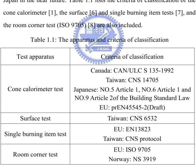
As becoming a member of WTO, the corresponding testing standards and classifications of Taiwan inevitably must harmonize with the ones that are popular adopted by the other countries. Although the cone calorimeter test method (CNS 14705) [11] has not become the legal criteria of classification yet in Taiwan, it is expected to be adopted like Japan in the near future. Table 1.1 lists the criteria of classification of the cone calorimeter [1], the surface [6] and single burning item tests [7], and the room corner test (ISO 9705) [8] are also included.

Table 1.1: The apparatus and criteria of classification Test apparatus Criteria of classification

Cone calorimeter test

Canada: CAN/ULC S 135-1992 Taiwan: CNS 14705

Japanese: NO.5 Article 1, NO.6 Article 1 and NO.9 Article 2of the Building Standard Law

EU: prEN45545-2(Draft) Surface test Taiwan: CNS 6532 Single burning item test EU: EN13823

Taiwan: CNS protocol Room corner test EU: ISO 9705

Norway: NS 3919

1.2 Literature review

(25)

done by Parker [12] on the ASTM E-84 tunnel test. Later, it was applied to a room fire test [13]. During the late of 70`s and early in 80`s this principle was refined at the National Institute of Standards and Technology (NIST). The first version of test standard of cone calorimeter (ASTM E1354) [4] was announced in 1990. ISO also announced the cone calorimeter test as ISO 5660 [1] and room corner test as ISO 9705 [8]. For ISO 5660 and 9705, the measurements and calculations of the heat release rate are similar, whereas the major difference is the magnitude of heat release rate which sustained.

Chen et al. [14] tested eighteen different wall-covering materials according to Chinese National Standard (CNS) 6532, equivalent to Japanese Industry Standard (JIS) A1321, and ASTM E1354 (Cone Calorimeter). A comparison of test results was presented, and a qualitative relationship was developed between the performances in the two methods.

Tsantaridis and Ostman [15] tested 30 products separately by cone calorimeter, SBI and room corner test. They found that the occurring times of the first peak of heat release rates for these three tests are in the good correlation. The comparisons of FIGRA (Fire Growth Rate) indices, defined in Chapter Two, of 30 products showed that the R2 of correlation between cone calorimeter and SBI is about 0.85, SBI and room corner test is about 0.92, and cone calorimeter and room corner test is about 0.76. The burning situation of materials in SBI was found very similar to that of Cone Calorimeter.

(26)

which are obtained from the full- and bench-scale tests, to consider the influence of the combustion conditions on the full scale smoke production. All these materials caused the occurrences of flashover within 10 min in the ISO Room Corner Fire Test. The smoke to heat ratio SQ (m2/MJ) was

used to compare smoke generation rates between these two tests. Plastics did produce more smoke yields than wood-based materials in both tests. However, no simple correlations were found between full scale and bench scale for smoke yield. An accurate empirical smoke prediction model by using bench scale fire parameters was presented to predict the full-scale smoke production rate at a heat release rate of 400kW.

Messerschmidt and Hees [17] studied the SBI tested data, which are obtained from fifteen laboratories of EU. They found that the test results for some materials tested in different laboratories show very different behaviors with each other. The reason discussed was the sensitivity of oxygen analysis instrument, indicating that the operation of oxygen analysis instrument must be careful in order to avoid the error.

Hakkarainen and Kokkala [18] developed a one-dimensional thermal flame spread model, which was used to predict the rate of heat release in the SBI test on the basis of the cone calorimeter data. The features of the measured and calculated heat release rate curves were compared for 33 building products. The fire growth rate indices (FIGRA) were calculated to predict the classification in the forthcoming Euroclass system. Although the model used cone calorimeter data could not simulate the heat release rate of SBI perfectly, the model still can provide the correct classification for 90% of the products studied.

(27)

Hees et al. [19] developed a prediction software tool by using the test data obtained from cone calorimeter (ISO 5660). The user-friendly software package, called cone-tools, allows users to predict the major classification parameters of HRR and FIGRA in the SBI and room corner tests. The results showed that the predictions are satisfactory, implying that the tool will be powerful for the product development by industry. Comparison between the SBI test results and data of cone-tools, it was shown that cone-tools could predict the accurate classification of EU up to 90%. Comparing with the room corner test results, the correction of prediction for the classification of EU was about 85%.

Axelsson and Hees [20] tested the sandwich panels, which were already tested from the previous Nordtest project. In that project, it was shown that the correlation between the SBI test method (EN 13823) and both the ISO 9705 and ISO 13784 part1 was insufficient. New data, tested by Axelsson and Hees on sandwich panels, were generated by using the European product standard prEN 14509. They were compared with ones from Nortest project. It showed that the correlation between the data from the full-scale test and SBI was not satisfactory. In addition, the SBI test method for sandwich panels would give irreproducible results so that the classifications could not reflect the real fire behaviors of the panels.

1.3 Scope of present study

This thesis intends to find the correlation among the fire performance tested data for the selected materials, which are measured from the Cone Calorimeter (in both vertical and horizontal positions),

(28)

Surface and Single Burning Item (SBI) tests. These measured data are analyzed in advance and then tried to correlate. Finally, the proper suggestions will be made for the fire performance criteria of classification for Taiwan according to these results.

(29)

Chapter Two

TEST APPARATUS AND EVALUATION

METHODS

This chapter will introduce four kinds of apparatus, which are the cone calorimeter, surface test, elementary materials test and SBI test, respectively, and their test procedures. The calculation methods for the Cone calorimeter and SBI tests are presented as well. Those fire parameters obtained from Cone calorimeter are especially crucial for the application of fire modeling.

2.1 Cone calorimeter

The ISO 5660[1] for cone calorimeter test is a bench-scale fire test method for assessing the contribution that the product tested can measure the rate of evolution of heat during its involvement in fire. The main parts of the apparatus are a cone-shaped radiant electrical heater with a temperature controller, spark igniter, weighing cell, holder of specimen, gas analyzer instrumentation, calibration equipment, smoke system and exhaust gas system. The picture and a schematic configuration of the cone calorimeter are presented in Figs. 2.1 and 2.2, respectively.

2.1.1 Introduction for cone calorimeter apparatus 2.1.1.1 Cone-shaped radiant electric heater

The electric heater is able to be of capable of horizontal or vertical orientation. The active element of the heater shall consist of an electrical heater rod, rated at 5kW at 240V, tightly wound into the shape of a

(30)

truncated cone (see Fig. 2.3). The heater is encased on the outside with a double-well stainless steel cone, packed with a refractory fiber material of approximately 100kg/m3 density. The irradiance from the heater is capable of being held at preset level by means of a temperature controller and three, type K, stainless steel sheathed thermocouples. The heater is capable of producing irradiances on the surface of the specimen of up to 100kW/m2. The irradiance is uniform within the central 50mm × 50mm area of the specimen, to within ± 2% in the horizontal orientation and to within ± 10% in the vertical orientation.

2.1.1.2 Load cell

The load cell for measuring specimen mass loss has an accuracy of 0.1g and it preferably has a measuring range of 500 g and a mechanical tare adjustment range of 3.5 kg.

2.1.1.3 Specimen holders

There are two kinds of specimen holders, horizontal and vertical orientations, showed in Figs. 2.4 and 2.5. The bottom of the holder is lined with a layer of density (nominal density 65kg/m3) refractory fiber blanket with a thickness of at least 13 mm. When testing on the horizontal orientation, the distance between the bottom surface of the cone heater and the top of the specimen is adjusted to 25 mm by using the sliding cone height adjustment. In the vertical orientation, the cone heater height is set so the centre lines up with the specimen centre. A retainer frame and wire grid are used when testing intumescing specimens in the horizontal orientation and can also be used to reduce unrepresentative edge burning of composite specimens and for retaining specimens prone

(31)

to delamination.

2.1.1.4 Exhaust gas system

The exhaust gas system with flow measuring instrumentation consists of a high temperature centrifugal exhaust fan, a hood, intake and exhaust ducts for the fan and an orifice plate flow meter. The exhaust system is capable of developing flows from 0.012m3/s to 0.035 m3/s. A restrictive orifice with an internal diameter of 57mm is located between the hood and the duct to promote mixing. A ring sampler is located in the fan intake duct for gas sampling, 685mm from the hood. The flow rate is determined by measuring the differential pressure across a sharp edge orifice (internal diameter 57mm) in the exhaust stack, at least 350mm downstream from the fan.

2.1.1.5 Gas analyzer instrumentation

The instrumentation incorporates a pump, a filter to prevent entry of soot, a cold trap to remove most of the moisture, a by-pass system set to divert all flow except that required for the oxygen analyzer and a further moisture trap. The detail part of instrumentation is shown in Fig. 2.6.

2.1.1.6 Smoke system

The smoke detection and measurement system employs a 0.5mW Helium-Neon laser operating at 632.8 nanometers. The laser system provides a means of obtaining the extinction coefficient based upon the degree of visual obscuration caused by suspended particulates in the exhaust stream.

(32)

2.1.1.7 Heater flux meter

The heater flux meter is the Gardon (foil) or Schmidt-Boelter (thermopiles) type with a design range of about 100kW/m2. The target receiving radiation, and possibly to a small extent convection, shall be flat, circular, of approximately 12.5 mm in diameter and coated with a durable matt black finish. The target shall be water-cooled. The instrument shall have an accuracy of within ±3% and the repeatability within 0.5%. It is positioned at a location equivalent to the centre of the specimen face in either orientation during this calibration.

2.1.1.8 Calibration burner

The burner is constructed from a square-section brass tube with a square orifice covered with wire gauze through which the methane diffuses. The tube is packed with ceramic fiber to improve uniformity of flow. The calibration burner is suitably connected to a metered supply of methane of at least 99.5% purity.

2.1.1.9 Optical calibration filter

Calibration of the smoke system is by operator insertion of pre-calibrated neutral density filters. Two high-quality optical filters of approximately 0.3 O.D. (Optical Density) and 0.8 O.D. are provided with precision fabricated keyed positioning holders. The manufacturer’s optical density curve is provided with each filter.

2.1.1.10 Ignition circuit

External ignition is accomplished by a spark plug powered from a 10 kV transformer. The spark electrode position is 13mm above the center of

(33)

the specimen in the horizontal orientation and 5mm above the top of the holder in the specimen plane in the vertical orientation.

2.1.2 Specimen construction and preparation for cone calorimeter 2.1.2.1 Specimens

Unless otherwise specified, three specimens shall be tested at each level of irradiance selected and for each different exposed surface.

The test specimen has an area of 100 mm × 100 mm and a maximum thickness of 50 mm. For products with normal thickness of greater than 50 mm, the requisite specimens shall be obtained by cutting away the unexposed face to reduce the thickness to 50±3 mm.

2.1.2.2 Conditioning of specimens

Before the test, specimens shall be conditioned to constant mass at a temperature of 23±2°C, and a relative humidity of 50±5% in accordance with ISO 554.

2.1.2.3 Preparation

A conditioned specimen is wrapped in a single layer of aluminum foil, of 0.03 mm to 0.05 mm thickness, with the shiny side towards the specimen, covering the unexposed surfaces. Composite specimens are exposed in a manner typical of the end-use condition. They are tested with the retainer frame and also prepared so that the sides are enveloped with the outer layer(s) or otherwise protected. If using retainer frame and wire grid, they shall be specified in the test report.

2.1.3 Test procedure for cone calorimeter

(34)

if necessary. Drain any accumulated water in the cold trap separation chamber. Adjust the distance between the bottom of cone heater and surface of specimen. This distance shall be 25mm.

2) Turn ON the computer and type CONE2A. The Calibrate & Test Specimens option allows operator to start the AutoCal cycle for complete system calibration prior to performing tests.

3) Turn ON all calibration gas, air, water and methane supplies. N2 gas

always shall be opened.

4) Change the Drierite, Ascarite and new 9cm filter if needed.

5) The computer program requests that all external exhaust blowers be turned off so a static pressure reading can be taken.

6) Turn ON external exhaust fans. The operator enters the desired Exhaust Flow Rate in m3/sec. Here we use 0.024m3/sec. When the reading is stable at the desired flow rate for 15 seconds, the AutoCal system will continue.

7) Choose YES or NO to use the last C factor. Select YES to use the last C factor. AutoCal will proceed to Heat Flux Calibration. Select NO to determine a new C factor. AutoCal will proceed to calibrate gas analyzers, smoke and weigh system to determining the new C factor. 8) For determining the new C factor, we first calibrate the laser system.

Insert the 0.8 O.D. filter and wait to read it completely. Repeat the procedure for the 0.3 O.D. filter.

(35)

specimen holder, without specimen, onto the weigh cell platform. 10) Enter the weight of the specimen holder and adjust the mechanical

tare for 0.00 ± 0.2 g.

11) With the specimen holder on the weigh cell, add a 500 gram mass. AutoCal will detect the mass and tale a Span reading. Don't remove the specimen holder. Remove the 500 gram mass.

12) The CONE2 will display this screen until the cold trap temperature reading is below 9°C before proceeding with the analyzer Span.

13) Remove the specimen holder and insert the calibration burner. Enter the desired Methane Flame Energy in the range of 3.5kW to 10kW. AutoCal will take a baseline oxygen reading and insert the spark igniter in preparation for methane flow. The nominal value of C factor should range from approximately 0.042 to 0.046.

14) Put the Heat Flux Transducer in place. Enter the desired heat flux level (0 to 100kW/m2) and the orientation for the test specimens. 15) Enter test information.

16) Start test. Insert the holder with specimen on the weigh cell platform and then press the START TEST button on the handset control.

17) When full flame ignition is observed, press and hold the FLAME VERIFICATION button on the handset. After the flame verification time has elapsed, the button will light up. Release the button and press SPARK OFF button to retract the spark.

(36)

cease and the average mass loss over a 1 min period has dropped below 150 g/m2. Press END TEST button.

2.1.4 Evaluation methods of cone calorimeter 2.1.4.1 The principle of Oxygen Consumption

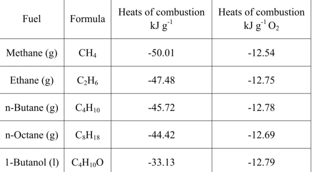
During 70’s to 80’s, a technique known as Oxygen Consumption Method was developed. It is a simple, versatile and powerful tool for estimating the rate of total heat release in fire tests. As early as 1917, Thornton [2] pointed out that the heats of combustion per unit mass of oxygen consumed for organic gases and liquids were approximately the same. Huggett [3] has examined a wide variety of fuels and concluded that Δh_c / r₀ = 13.1 MJ/kg O2 represents a value typical of most

combustibles, including gases, liquids, and solids. To implement this principle it would be necessary only to measure the total mass flow of oxygen in the combustion products and to compare that to the initial inflow, that is

(

₂_, ₂

)

0 O O c _m _m r h

q&= Δ & _∞ − & (2.1)

where the subscript ∞ denotes baseline ambient condition prior to start of test. From the form of this expression it can be seen that it does not matter at what speed the products are exhausted or how much excess air is pulled through. It is as if we were interested only in counting oxygen “holes＂. Some of the typical values of heat of combustion per unit mass of oxygen consumed are listed in the Table 2.1 to 2.3.

(37)

2.1.4.2 Calibration Factor (C factor)

The methane calibration shall be performed daily to check for the proper operation of the instrument and to compensate for minor changes in determination of mass flow.

(

3

)

(

)

0₂ ₂ 2 5 . 1 105 . 1 10 . 1 10 54 . 12 0 . 10 O O O e p T C

χ

− − Δ × = (2.2) The calibration constant C, is calculated using equation (2.2), where 10.0kW methane supplied, 12.54×103KJ /Kg value of heat of

combustion per unit mass of methane consumed and 1.10 is the ratio of the molecular weights of oxygen and air.

2.1.4.3 Heat Release Rate

Prior to performing other calculations, calculate the oxygen analyzer time shift, td, using the following equation:

( )

O

(

d

)

O t = t +t 1 2 2

χ

(2.3) Calculate the heat release rate, q&

( )

t :

( )

(

)

( )

_{( )}

t t T p C r h t q O O O e c 2 2 2 5 . 1 105 . 1 10 . 1 0 0

χ

− − Δ ⎟⎟ ⎠ ⎞ ⎜⎜ ⎝ ⎛ Δ = & (2.4)

Heat release rate per unit area can then be obtained:

( ) ( )

t q t A_s

q&′′ = & / (2.5)

(38)

( )

t t q q i i′′ Δ = ′′

_∑

_& (2.6) where 0 r h_c Δ

is 13.1kJ/kg, value of heat of combustion per unit mass of oxygen consumed.

2.1.4.4 Mass Loss Rate of Specimen

Evaluation of mass loss rate of testing specimen is necessary for providing information like critical mass loss rates for ignition and extinction, yielding of gaseous products and effective heat of combustion. The mass loss rate is calculated numerically by a five-point approximation method with a given Δt_{time interval.}

For the first scan i=0,

t m m m m m dt dm i Δ + − + − = ⎥⎦ ⎤ ⎢⎣ ⎡ − = 12 3 16 36 48 25 ₀ ₁ ₂ ₃ ₄ 0 (2.7)

For the second scan i=1,

t m m m m m dt dm i Δ − + − + = ⎥⎦ ⎤ ⎢⎣ ⎡ − = 12 6 18 3 10 ₀ ₁ ₂ ₃ ₄ 1 (2.8) For scan i=1<i<i=n−1, t m m m m dt dm _i _i _i _i i Δ + − + − = ⎥⎦ ⎤ ⎢⎣ ⎡ − − − + + 12 8 8 ₁ ₁ ₂ 2 _(2.9) For scan i= n−1,

(39)

t m m m m m dt dm _n _n _n _n _n n i Δ + − + − − = ⎥⎦ ⎤ ⎢⎣ ⎡ − − − − − − = 12 6 18 3 10 ₁ ₂ ₃ ₄ 1 (2.10)

For last scan i= , n

t m m m m m dt dm _n _n _n _n _n n i Δ − + − + − = ⎥⎦ ⎤ ⎢⎣ ⎡ − − − − − = 12 3 16 36 48 25 ₁ ₂ ₃ ₄ (2.11) 2.1.4.5 Effective Heat of Combustion

The averaged effective heat of combustion can be determined as

( )

f i i eff c m m t t q h − Δ = Δ _,

∑

& (2.12)

( )

⎟ ⎠ ⎞ ⎜ ⎝ ⎛ − Δ = Δ ⇒ dt dm t t q t h_c_,_eff &i (2.13)

where minitial and mfinal are mass of specimen at ignition and extinction,

respectively. 2.1.4.6 Smoke

Extinction Coefficient K [1/m] is determined by laser intensity.

I I L K 1⎟ln 0 ⎠ ⎞ ⎜ ⎝ ⎛ = (2.14) ( ) f i i i i i avg f m m t K V − Δ =

∑

& &

σ

(2.15)

(40)

2.2 The surface and elementary material tests

The Chinese National Standard (CNS) 6532, assigned in the building code for Taiwan, is a bench-scale test for interior finish materials. It includes two test procedures: a surface test, which is compulsory, and an elementary material test. Whether the latter has to be performed depends on the result of the surface test. The apparatus for the surface test mainly consists of a smoke accumulation box, a furnace and an optical density-measuring system; see Fig. 2.7.

2.2.1 Introduction for the surface test apparatus 2.2.1.1 Furnace

The furnace is shown in Fig. 2.8. There are two quartz lamps, a propane burner, a thermocouple to measure back-face temperature of specimen and two thermocouples to get exhaust temperature of specimen in the furnace. In the furnace, heat is provided by a T-shaped propane burner, with a flow rate of 0.35 1/min for the first 3 mins, subsequently, an additional heat is supplied by two quartz lamps (total output is 1.5kW). The history of average value of heat flux is shown in Fig. 2.9, which is adopted from [14]. In the first 3 mins, the average value of heat flux is 0.49kW/m2 and at the 10 mins it is 13.71kW/m2. As to the theoretical value, it is 14.15kW/m2 for the first 3 mins.. After that, the theoretical value of total heat flux is 60.45kW/m2. The detailed calculation of theoretical value of heat flux is given in Appendix A. The tremendous discrepancy between the theoretical value and measurement is attributed to the neglected convectional effect, which is existed in the experiment, on the theoretical computation. The total heating time for fire-retardant

(41)

materials is 6 mins. For non-combustible and semi-combustible materials, it is 10 mins.

2.2.1.2 Smoke accumulation box

The smoke accumulation box (see Fig. 2.10) measures 1.41 m x 1.41 m x 1.0 m (Width x length x height) and is equipped with a stirrer to make the smoke homogenous distributed.

2.2.1.3 Optical density-measuring system

The capacity of smoke flow is about 1.5L/min. The light source is a halogen light. The device is shown in Fig. 2.11.

2.2.2 Specimen preparation for the surface test 2.2.2.1 Specimens

The test specimen must be the same as the one in end-use. Six specimens are provided and three of them are randomly chosen to test. The area of specimen is 220 mm × 220 mm and its thickness is the same as the original one. The heating zone is 180 mm × 180 mm. For the standard-testing material (Pearlite board), its dimension is 220 mm ×

220 mm × 10 mm.

2.2.2.2 Conditioning of specimens

The testing specimens should be put in the ventilated room for more than one month. Just before the test, specimens shall be dried more than 24 hours in an oven and then they are put it into a dry box more than 24 hours. The temperature of oven is about 40 ± 5°C. In addition, the pearlite board shall be dried in the oven for more than 72 hours and then putd it into dry box for more than 24 hours.

(42)

The surface lining material is installed into the furnace and the backboard with a thermocouple is put tightly behind the specimen.

2.2.3 Test procedure for surface test

1) Turn on all power sources, which included Logarithmic Converter, smoke agitator and computer. Wait for over 30 mins to stabilize. The smoke agitator shall be always opened.

2) On the Logarithmic Converter, choose the “OFF” and set the value of CA as zero.

3) On the same Converter, choose the “MEAS” and zero the value of CA.

Then choose the “CA set” and adjust the value of CA to 240.

4) Repeat the third step until the value of CA becomes steady and then

choose the “MEAS”.

5) Adjust the flow of propane to about 0.35 L/min.

6) Preheat two quartz lamps. First heat them for 15 mins by using 1.0 kW and then turn off the power for 10 mins. After that, heat them for 10 mins by using 1.5 kW and then turn off the heater to complete the preheating.

7) The exhaust valve of smoke shall be closed during the test. 8) Wait the exhaust temperature to drop to the atmosphere value.

9) Pearlite board shall be tested first to get the reference curve. The error of temperature per min is tolerated up to about ± 20°C.

(43)

10) Key the information data of specimen into the computer and start the test.

11) Observe the sustained flaming and cracks in the back surface after completion of the test. And then open exhaust valve of smoke.

2.2.4 Evaluation methods of the surface test

Typical temperature and smoke-generation curves, together with the standard curves are shown in Fig. 2.12. The standard temperature curve is obtained by adding 50°C to the calibration curve. One of the results from each test is the tdΘ value, which is a measurement of increase in temperature. The tdΘ value is equal to the area under the test and the standard temperature curves. If the former is always below the latter during the heating period, tdΘ is equal to zero. The time when the two curves intersect, tc, must always be greater than 3 mins. If this is not the

case, the material fails and is unclassified according to CNS 6532.

The coefficient of smoke generation, CA, is calculated by measuring

the intensity of the light transmitted through the smoke flow before the test, I0, and during the test, I. When these values are obtained, CA value is

calculated using the following expression:

I I

C_A =240⋅log 0 (2.16)

where I0 = Intensity of the light before the test (LUX)

(44)

2.2.5 An elementary material test

The elementary material test apparatus is almost similar to the ISO test apparatus, see Fig. 2.13. The test is only used when the requirements in the surface test for a non-combustible material are met. The test apparatus can provide a high temperature environment, equivalent to the fully developed fire, to estimate the fire protection of entire specimen.

The specimens are piled up to (40± 2 mm) × (40± 2 mm) ×

(50± 2 mm), which are cut from building material. Three specimens shall be prepared. The conditioning process is the same as that for surface test.

Test procedure for the elementary material test is described as follows. It must be preheated at first. During preheating procedure a firebrick shall be suspended in the furnace all the time. Total preheated time is about 3 hours that the resultant hot environment inside the furnace is 750°C. Specimens are subjected to a 750°C furnace environment for 20 min when the furnace maintains 750°C for 20 mins in advance. The temperature difference shall be observing during the test.

2.3 SBI test

The SBI test is an intermediate scale test which consists of a compartment surmounted by a small calorimeter hood, which is connected to a calorimeter duct via a mixing box and baffles. The pictures are shown in Figs. 2.14 and 2.15. The specimen is a corner section and is positioned on a trolley (see Fig. 2.16) that can insert into the compartment. The compartment is positioned within a 3 m × 3 m ×

(45)

2.6 m test room.

2.3.1 Introduction for SBI apparatus

2.3.1.1 Burners and propane supply system

The SBI apparatus contains two identical sandbox burners, one in the bottom plate of the trolley (the main burner), one fixed to a post of the frame (the auxiliary burner). The main burner is mounted in the tray and connected to the U-profile at the bottom of the specimen position. The top edge of the main burner is at 10 mm above the trolley floor level. The auxiliary burner is fixed to the post of the frame opposite to the specimen corner, with the top of the burner at a height of 1450 mm from the floor.

The specimens are protected from the heat flux of the flames of the auxiliary burner by a shied of rectangular shape, width 350± 5 mm, height 550 ± 5 mm, made of calcium silicate board (backing boards).

The burners are equipped with an ignition glow plug. There is a solenoid valve for immediate and automatic cut-off of the gas supply in case of extinction of the main or auxiliary burners which is detected via two UV detectors. The propane controller is housed in the Gas Diverter (see Fig. 2.14) on the outside of the room. The switch used to supply propane to one of both burners is operated by Gas Control Box (see Fig. 2.17).

2.3.1.2 Smoke Exhaust system

Under test conditions, the smoke exhaust is capable of continuously extracting a volume flow, normalized at 298 K, of 0.5 - 0.65m3/s. The system are shown in Figs. 2.18 and 2.19.

(46)

2.3.1.3 General measurement section equipment

The general measurement section of the exhaust tube contains, among others, three thermocouples, a bi-directional probe, a gas sampling probe, and a light attenuation measurement system.

Three thermocouples, all of the K-type in accordance with EN 60584-1, diameter 0.5mm sheathed and insulated.

The bi-directional probe is connected to a pressure transducer with a range of 0-100Pa and an accuracy of ± 2Pa. The pressure transducer, primary filter and air flow meter for the smoke measurement system are located on the Filter Panel, situated next to the Measurement Section.

The gas sampling is connected to a gas conditioning unit and gas analyzers for O2 and CO2 housed in the FTT Gas Analysis Rack. The O2

analyzer is of the paramagnetic type, and meets the specification of EN 13823, with a range of 0% - 21% oxygen, an absolute accuracy of 0.05% (VO2/Vair). The CO2 analyzer is of the IR type, with a range of 0% - 10%

carbon dioxide, with an absolute accuracy of 0.1% (VCO2/Vair).

2.3.1.4 Smoke measurement system

The smoke measurement system consists of lamp, lens system and detector. A lamp is incandescent filament type and operating at a color temperature of 2900± 100 K. A lens system to align the light is a parallel beam.

2.3.1.5 Data acquisition system

The signals are collected using a HP Data Acquisition / Switch Unit. A screen based software package enables simple data acquisition and

(47)

analysis to determine the various parameters needed for heat release determination. It generates files that integrate with the current TNO spreadsheet, (which are also supplied) so that the Fire Growth Rate Index (FIGRA) and Smoke Growth Rate Index (SMOGRA) can be calculated. 2.3.2 Specimen construction and preparation of SBI test

2.3.2.1 Specimens

The corner specimen consists of two wings, designated the short and long wings respectively. The dimensions of the short wing are (495± 5) mm × (1500 ±5) mm. The dimensions of the long wing are (1000 ±5) mm × (1500 ±5) mm. The maximum thickness of a specimen is 200mm. Specimens with a thickness of more than 200mm shall be reduced to a thickness of 200mm by cutting away the unexposed surface.

2.3.2.2 Backing Boards

The backing boards is calcium silicate boards with a density of (800± 150) kg/m3_{and a thickness of (12}_{± 3) mm. The dimensions of the}

short wing shall be (at least 570mm + width of specimen) mm × (1500± 5) mm. The long wing shall be (1000 ± 5) mm × (1500± 5) mm. Three specimens (three sets of ling plus short wing) are needed.

2.3.2.3 Condition of specimens

The parts that compose a specimen may be conditioned separately or fixed together. However, specimens that tested glued to a substrate shall be glued before conditioning. The entire procedure is carried out within 2h of removal of the specimen from the conditioning environment.

(48)

The specimen wings are placed in the trolley. First the short wing specimen and backing board are placed on the trolley, with the bottom edge of the specimen against the short U-profile on the trolley floor. Next the long wing specimen and backing board are placed on the trolley. Both wings are wedged at the top and the bottom. Be sure that the corner line of the backing boards does not widen during the test.

2.3.3 Test procedure for SBI

1) Check trolley shall be installed into the test room. Connect two lines of Gas Diverter and open two valves. Replace the sorbents if necessary. Close the door of test room. Open the propane gas.

2) Push the Analyzers button of Gas Analysis Rack and Power On button of Gas Control Box.

3) Push the Cold Trap button of Gas Analysis Rack. Open the computer and run the software of SBICalc.

4) There are 9 buttons displayed across the button of the screen. Choose the Calibrations and All transducers.

5) Zero DPT and SMOKE (No light, 0%) on software. 6) Push the Smoke button of Gas Analysis Rack.

7) Open an exhaust fan. Under ambient conditions, the volume flow shall be normalized about 0.6m3/s.

8) Push the Gas On button of the Gas Control Box. The Interlocks Made on the Gas Control Box shall be green light.

(49)

9) Zero MFM and push the OK button to save the settings.

10) Open N2 gas and turn two valves of the Rack to Nitrogen. Wait for

five minutes.

11) Zero O2 on analyzers. (Password : 4000)

12) Zero O2 on software and push the OK button to save settings.

13) Zero CO2 on analyzers. Zero CO2 on software.

14) Zero CO on analyzers. Zero CO on software and push the OK button to save settings.

15) Close the N2 gas. Open the CO/CO2 gas and turn two valves of the

Rack to Air and CO/CO2. Wait for five minutes.

16) Span CO2 on analyzers and Span CO2 on software.

17) Span CO SPAN CO on analyzers and Span COon software.

18) Close CO/CO2 gas. Turn two valves of the Rack to Air and Sample

gas.

19) Push the Pump button and wait for 5-10 minutes. 20) Span O2 on analyzers and Span O2 on the software.

21) Span Smoke (Light, 100%) on software and save settings. 22) Enter test information, included humidity.

23) Start the test. When t = (120± 5) s, auxiliary burner shall be ignited. Adjust the propane mass flow m gas to (647 ±5) mg/s. The time

(50)

of heat release.

24) When t = (300 ±5) s, the propane supply from the auxiliary burner to the main burner shall be switched.

25) Observe the burning behavior of the specimen for a period of 1260 s and record the data on the record sheet. The nominal exposure period of the specimen to the flames of the main burner is 1260 s. The performance is evaluated over a period of 1200 s.

26) After t = 1560 s, the end of test conditions on the record sheet at least 1 min shall be recorded, without the influence of remaining combustion. If the specimen is difficult to extinguish totally, the trolley may need to be removed.

2.3.4 Evaluation methods of SBI test

2.3.4.1 Calculation of heat release rate (HRR)

2.3.4.1.1 Total HRR of specimen and burner: HRR total

a) Calculation of the volume flow of exhaust system, normalized at 298 K, V298(t):

( )

_{( )}

t T t p k k cA t V ms t Δ = ρ 298 (2.17)

b) Calculation of the oxygen depletion factor

φ

( )

t :

( )

(

)

{

₍

( )

₎

_{

}

( )

_{( )}

{

_{( )}

_}

(

)

}

t xO t xCO s s O x s s CO x t xO t xCO s s O x t 2 2 2 2 2 2 2 1 90 ... 30 90 ... 30 1 1 90 ... 30 − − − − − =

φ

(2.18) c) Calculation of 2 _ O a x :

(51)

(

)

₍

₎

_⎥ ⎦ ⎤ ⎢ ⎣ ⎡ ⎭ ⎬ ⎫ ⎩ ⎨ ⎧ − − − = 46 90 ... 30 3816 2 . 23 exp 100 1 90 ... 30 2 _ ₂ s s T p H s s O x x ms O a (2.19) d) Calculation of HRR_total

( )

t [kW]:

( )

_{( )}

⎟ ⎠ ⎞ ⎜ ⎝ ⎛ + = t t x t EV t HRR_total _a _O

φ

105 . 0 1 2 _ 298 (2.20) 2.3.4.1.2 HRR of the burner

The HRR_burner

( )

t is equal to HRR_total

( )

t during the base line period. The average HRR of the burner is calculated as the average HRR_total

( )

t during the base line period

(

210s≤t ≤270s

)

:

(

s s

)

HRR

HRR_av_{_}_burner = total 210 ...270 (2.21) where HRRav_burner is the average heat release rate of the burner [kW].

The criteria of HRR_av_{_}_burner shall meet the value, 30.7±2.0kW .

2.3.4.1.3 HRR of the specimen

In general, the heat release rate of the specimen is taken as the total heat release rate HRR_total

( )

t minus the average heat release rate of the burner HRR_av_{_}_burner : For t > 312s,

( )

burner av total t HRR HRR t HRR = − _{_} (2.22) where HRR(t) is the heat release of the specimen [kW].

(52)

of the exposure period, the total heat output of the two burners is less than HRRav_burner. For t = 300s, HRR(300s) = 0 kW For300s<t≤312s_,

( )

{

( )

}

burner av total t HRR HRR t HRR =max.0, − _{_} (2.23) 2.3.4.2 Calculation of THR(t) and THR600s

The total heat release of the specimen THR(t) [MJ] and the total heat release of specimen in the first 600s of the exposure period

(

300s≤t≤900s

)

, THR600s , are calculated as follows:

( )

=

_∑

ta

( )

s a HRR t t THR 300 1000 3 (2.24)

( )

∑

= s s s HRR t THR 900 300 600 ₁₀₀₀ 3 (2.25)

where the factor 3 is introduced since only one data point is available every three seconds.

2.3.4.3 Calculation of FIGRA0.2MJ and FIGRA0.4MJ

The FIGRA (fire growth rate indices) [W/s] are defined as the maximum of the quotient HRRav

( ) (

t / t−300

)

, multiplied by 1000. The quotient is calculated only for that part of the exposure period in which the threshold levels for HRRav and THR have been exceeded. If one or

both threshold values of a FIGRA index are not exceeded during the exposure period, that FIGRA index is equal to zero. Two different

(53)

THR-threshold values are used, resulting in FIGRA0.2MJ and FIGRA0.4MJ.

a) Calculate FIGRA0.2MJ for all t where:

(HRRav(t) > 3 kW) and (THR(t) > 0.2 MJ) and 300s<t≤1500s;

b) Calculate FIGRA0.4MJ for all t where:

(HRRav(t) > 3 kW) and (THR(t) > 0.4 MJ) and 300s<t≤1500s; Both using:

( )

⎟ ⎠ ⎞ ⎜ ⎝ ⎛ − × = 300 max 1000 t t HRR FIGRA av (2.26)

2.3.4.4 Calculation of smoke production rate (SPR) 2.3.4.4.1 Total SPR a) Calculation of V(t) [m3/s]:

( )

( ) ( )

298 298 t T t V t V = ms (2.27) b) Calculation of SPRtotal(t) [m2/s]:

( )

(

_{( )}

)

_⎥ ⎦ ⎤ ⎢ ⎣ ⎡ = t I s s I L t V t SPR_total ln 30 ...90 (2.28) 2.3.4.4.2 SPR of the burner

The smoke production rate of the burner is equal to SPRtotal(t) [m2/s]

during the base line period. The average SPR of the burner is calculated as the average SPRtotal(t) during the base line period

(

210s≤t ≤270s

)

:

(

s s

)

SPR

創新建材在圓錐量熱儀、表面測試爐及單材耐燃測試儀之火災試驗數據相關性之研究

國 立 交 通 大 學

機械工程學系

碩士論文

創新建材在圓錐量熱儀、表面測試爐及

單材耐燃測試儀之火災試驗數據相關性

之研究

The Research for Testing Data Correlation

of New and Innovative Building Materials

between the Cone Calorimeter, the Surface

and SBI Tests

研究生 ：戴嘉鴻

指導教授 ：陳俊勳 教授

摘要

Abstract

誌謝

CONTENTS

LIST OF TABLES

LIST OF FIGURES

Appendix

Nomenclature

χ

χ

χ

σ

(

)

( )

( )

( )

(

)

( )

( )

( )

( )

φ

Chapter One

INTRODUCTION

Chapter Two

TEST APPARATUS AND EVALUATION

METHODS

(

)

(

)

(

)

χ

χ

χ

( )

(

)

χ

χ

( )

( )

(

)

( )

( )

χ

χ

χ

( ) ( )

( )

∑

( )

∑

( )

( )

∑

σ

( )

( )

( )

φ

( )

( )

國立交通大學

研究生：戴嘉鴻

指導教授：陳俊勳教授

_{( )}

_∑

_{( )}

₍

₎

_{

_{( )}

_{( )}

_}

₍

₎

_{( )}

_∑

_{( )}