國 立 交 通 大 學
資 訊 科 學 與 工 程 研 究 所
博 士 論 文
多重輸入輸出正交分頻多工基頻收發機
之設計與實現
Design and Implementation of a MIMO-OFDM
Baseband Transceiver
研 究 生 : 孫明福
指導教授 : 許騰尹
多重輸入輸出正交分頻多工基頻收發機
之設計與實現
Design and Implementation of a MIMO-OFDM
Baseband Transceiver
研 究 生:孫明福
Student: Ming-Fu Sun
指導教授:許騰尹 博士
Advisor: Dr. Terng-Yin Hsu
國 立 交 通 大 學
資 訊 科 學 與 工 程 研 究 所
博 士 論 文
A Dissertation
Submitted to Department of Computer Science College of Computer Science
National Chiao Tung University in Partial Fulfillment of the Requirements
for the Degree of Doctor of Philosophy in
Computer Science June 2009
Hsinchu, Taiwan, Republic of China
多重輸入輸出正交分頻多工基頻收發機
之設計與實現
孫明福
國立交通大學資訊科學與工程研究所
指導教授:許騰尹教授
摘要
本研究探討了4×4 多重輸入輸出正交分頻多工無線通訊系統與進階的接收技術,其 中包含了抗I/Q 不平衡效應的自動頻率調整器、訓練序列輔助的 I/Q 不平衡效應偵測、 適應性通道偵測、以及數位波束成型。 為了偵測在I/Q 不平衡效應干擾下的載波頻率偏移量,發展了一個基於虛擬載波頻 率偏移技巧的載波頻率偏移偵測演算法。此演算法透過注入虛擬的載波頻率於三個連續 的訓練序列來改善載波頻率偏移偵測的精準度。從模擬的結果中,演算法的偵測錯誤量 大約是0.3 ppm,並且低於傳統載波頻率偏移偵測演算法。透過 0.13-μm CMOS 製程, 此演算法實現在一個測試晶片上。此測試晶片的面積為3.3×0.4 mm2,耗電量為10 mW。 在直接降頻的架構下,必須同時考慮頻率相關I/Q 不平衡與載波頻率偏移效應。本 文提出一個利用訓練序列來偵測載波頻率偏移干擾下的I/Q 不平衡效應。在載波頻率偏 移干擾下的頻率相關 I/Q 不平衡效應可透過資料子載波與干擾子載波之間的關係偵測 出來。模擬與實驗平台的結果顯示提出的方法可以有效改善系統效能。此外本文所提出 的方法也相容於目前的無線區網標準。 最近對於移動下的無線通訊需求有增加的趨勢。為了達到高效能的接收機,就需要 具備快速的通道追蹤能力。越快取得精確的通道狀態資訊並達到成功的傳輸是非常重要 的。針對4×4 多重輸入輸出正交分頻多工無線通訊系統,我們發展一個在時變通道下的 適應性頻域通道偵測器。此適應性頻域通道偵測器利用每四組符號來確保通道偵測的精 準度。為了降低硬體複雜度,利用了Alamouti 矩陣的特性來設計有效率的 VLSI 架構。最後透過0.13-μm CMOS 製程,此適應性頻域通道偵測器的面積為 3×3.1 mm2,另外4×4 多重輸入輸出正交分頻多工無線通訊系統晶片在1.2V 電壓下耗電量為 62.8 mW。 此外,本研究也探討了數位波束成型在多重輸入輸出正交分頻多工通訊系統上的應 用。數位波束成型是一種方向性濾波的技術,能有效的消除不必要的干擾,並正確的接 收訊號。因此,數位波束成型技術可用來增加系統的容量與傳輸距離。 本研究探討收發機設計與元件實作。此外也建構了一個基於軟體定義的收發機平台 來提供快速的原型機驗證。透過整體的效能指標評估,可在實作權衡上有效取得平衡。
Design and Implementation of a MIMO-OFDM
Baseband Transceiver
by
Ming-Fu Sun
Department of Computer Science
National Chiao Tung University
Advisor: Terng-Yin Hsu
Abstract
In this study, a 4 4× multi-input multi-output (MIMO) orthogonal-frequency division multiplexing (OFDM) communication system and advanced receiving techniques, including anti-I/Q mismatch (IQ-M) auto frequency controller, preamble-assisted IQ-M estimator and compensator, adaptive channel estimator, and digital beamforming are explored.
In order to estimate the carrier frequency offset (CFO) value under the conditions of IQ-M for direct-conversion structures, a pseudo-CFO (P-CFO) algorithm is developed. The proposed P-CFO algorithm rotates three training symbols by adding extra frequency offset into the received sequence to improve CFO estimation. Simulation results indicate that the estimation error of the proposed method is about 0.3 ppm, which is lower than those of two-repeat preamble-based methods. The proposed scheme is implemented as part of an OFDM wireless receiver fabricated in a 0.13-μm CMOS process with 3.3 0.4× mm2 core area and 10 mW power
consumption.
must be considered. A preamble-assisted estimation is developed to circumvent the frequency-dependent IQ-M with CFO. The frequency-dependent IQ-M with CFO can be estimated by taking advantage of the relationship between desired sub-carriers and image sub-carriers. Both simulation and experiment results indicate that the proposed method can meet system requirements by preventing frequency-dependent IQ-M from significantly degrading the performance. Moreover, the proposed scheme is compatible with current wireless local area network standards.
Recently, the request for wireless communication under mobile conditions is increased. The ability of fast channel tracking is therefore needed to achieve high performance receivers. For successful transmissions, obtaining accurate channel state information as soon as possible is extremely important. An adaptive frequency-domain channel estimator (FD-CE) for equalization of 4 4× MIMO-OFDM system in time-varying frequency-selective fading is developed. The proposed adaptive FD-CE ensures the channel estimation accuracy in each set of four MIMO-OFDM symbols. To decrease complexity, the rich feature of Alamouti-like matrix is exploited to derive an efficient VLSI solution. Finally, this adaptive FD-CE using an in-house 0.13-μm CMOS library occupies an area of 3 3.1× mm2, and the 4×4 MIMO-OFDM modem consumes
about 62.8 mW at 1.2V supply voltage.
In addition, digital beamforming for MIMO-OFDM communications is also studied. Digital beamforming is a method of spatial filtering, which can eliminate unwanted interferences and receive desired signal accurately. Consequently, digital beamforming can be used to increase system capacity and transmission range.
In this study, the transceiver design and circuit implementation are presented. A software-defined radio is also constructed for rapid verification and fast prototyping. Based on the overall system performance index, the implementation trade-offs can be balanced.
Acknowledgments
This dissertation describes the research work I performed in the Integration System and Intellectual Property (ISIP) Laboratory during my graduate studies at National Chiao Tung University. This work would not be possible without the support of many people. I would like to express my most sincere gratitude to all those who have made this possible.First of all, I would like to thank Prof. Terng-Yin Hsu for the advice, guidance, and funding he has provided me with. I feel honored by being able to work with him. I would like to thank the committee members for their contribution for reviewing the manuscript and providing me with valuable feedback.
I would like to warmly thank many of present and former ISIP members: You-Hsien Lin, Wei-Chi Lai, Ta-Yang Juan, Shih-Lin Lo, Frank Hsiao, Jin-Hwa Guo, Chueh-An Tsai, Ming-Yeh Wu, Ming-Feng Shen, Li-Sheng Lu, Jyun-Rong Li, Hsin-Nan Chen, Kan-Si Lin, I-Yin Liu, Chuen-Tai Wang, Cheng-Yuan Lee, Yen-Her Chen, Shao-Hung Lu, and Chang-Ying Chuang, whose contributions were instrumental in the development of ideas. I also want to thank Min-Zheng Shieh, Ja-Hsing Kao, and Chon-Jei Lee for their friendship.
In addition, I gratefully acknowledge the constructive comments provided by Dr. Chien-Ching Lin and the wisdom of life experience shared by Prof. Terng-Ren Hsu.
Most of all, I am indebted to my family for their unconditional love and support they provide me with. It means a lot to me.
Ming-Fu Sun
Table of Contents
List of Tables
xi
List of Figures
xii
List of Acronyms
xvi
Chapter 1 Introduction
1
1.1 Motivation... 1
1.2 Dissertation Overview... 4
Chapter 2 Overview of MIMO-OFDM Systems
7
2.1 MIMO Wireless Communications... 72.1.1 Antenna Configurations... 7
2.1.2 Capacity Results... 9
2.1.3 Space-Time Processing... 11
2.1.4 MIMO-OFDM Systems... 15
2.2 Non-Ideal Front-End Effects... 16
2.2.1 Effects of Carrier Frequency Offset... 17
2.2.2 Effects of I/Q Mismatch... 23
2.2.3 Effects of Non-linearity... 27
2.2.4 DC Offset... 29
2.2.5 Quantization Noise and Clipping... 30
2.3 Wireless Channel Models... 32
2.3.1 AWGN... 32
2.3.2 Multipath... 34
2.3.3 MIMO Channel: TGn Channel Model... 36
Chapter 3 Anti-I/Q Mismatch Auto Frequency Controller
39
3.1 System Model... 42
3.2 Estimation for Carrier Frequency Offset... 44
3.2.1 Conventional Algorithm... 44
3.2.2 The Proposed Pseudo CFO Algorithm... 48
3.3 Simulation and Performance... 53
3.4 Implementation Hints... 60
3.4.1 Design Methodology... 60
3.4.2 Architecture of P-CFO Algorithm... 61
3.4.3 Verification Platform... 64
3.5 Summary... 67
Chapter 4 Preamble-Assisted Estimation for I/Q Mismatch
69
4.1 System Model... 714.2 Constant IQ-M Estimation... 74
4.2.1 Constant IQ-M Estimation without CFO... 74
4.2.2 Constant IQ-M Estimation with CFO... 79
4.3 Frequency-Dependent IQ-M Estimation... 87
4.3.1 The Proposed Method... 87
4.3.2 Simulation and Experiment Results... 91
4.4 Transmitter IQ-M Estimation... 97
4.4.1 Problem Statement... 97
4.4.2 The Proposed Method... 99
4.5 Summary... 104
Chapter 5 Adaptive Channel Estimation
105
5.1 System Description and Problem Statement... 1085.1.1 Modem Specification... 108
5.1.2 Problem Statement... 109
5.2 STBC Decoder and Equalization... 110
5.3 The Proposed Method... 112
5.3.1 Adaptive Frequency-Domain Channel Estimator... 112
5.3.2 Discussion... 118
5.4 Performance Evolution... 122
5.5.1 Proposed Architecture... 123
5.5.2 Implementation Results... 130
5.6 Summary... 133
Chapter 6 Digital Beamforming
135
6.1 The Basics of Digital Beamforming... 1366.2 Angle-of-Arrival Estimation... 140
6.2.1 Capon AOA Estimate... 142
6.2.2 MUSIC AOA Estimate... 145
6.3 Array Factor Calculation... 147
6.4 Digital Beamforming in MIMO Transmission... 154
6.5 Summary... 157
Chapter 7 Conclusion
159
7.1 Summary... 159 7.2 Future Work... 161References 165
Appendix A Derivation of (2.15)
175
Appendix B Derivation of (3.13)
179
Appendix C Derivation of (4.12)
181
Appendix D Supplementary of OFDM-Based System Specification 183
D.1 SISO-OFDM Systems... 183 D.1.1 Air Interface... 183 D.1.2 Major Parameters... 184 D.1.3 Frame Structure... 186 D.2 MIMO-OFDM Systems... 188 D.2.1 Air Interface... 188 D.2.2 Major Parameters... 189 D.2.3 Frame Structure... 192Appendix E Some Circuit Implementation Issues
194
E.1 Complex Multiplier... 194E.2 Fast Fourier Transform... 195
E.3 Numerically Controlled Oscillator... 197
About the Author
200
List of Tables
TABLE 2-1 AM-AM and AM-PM Models... 28
TABLE 3-1 Simulation Parameters... 55
TABLE 3-2 Required SNR... 60
TABLE 3-3 Complex Multiplier... 62
TABLE 3-4 The Complexity (Gate Count) of P-CFO... 62
TABLE 3-5 Chip Summary... 63
TABLE 4-1 Experiment Parameters... 93
TABLE 5-1 Operation of the Adaptive FD-CE... 117
TABLE 5-2 Experimental Parameters... 132
TABLE 5-3 Synthesized Results (Gate Count)... 132
TABLE 5-4 Chip Summary of The 4 4× MIMO-OFDM Modem... 132
TABLE 6-1 Weight Vectors for the Two-Element Array... 152
TABLE 6-2 Weight Vectors for the Four-Element Array... 152
TABLE D-1 Modulation Parameters... 185
TABLE D-2 Timing Related Parameters... 186
TABLE D-3 Modulation Parameters... 191
TABLE D-4 Timing Related Parameters... 192
TABLE F-1 Fourier Transforms... 199
List of Figures
Figure 1-1 Data rate versus mobility of wireless communication standards... 2
Figure 2-1 Different antenna configurations... 8
Figure 2-2 Block diagram of the MIMO system... 10
Figure 2-3 Block diagram of the 2 2× MIMO system with Alamouti’s scheme... 12
Figure 2-4 Space-time block code in the MIMO-OFDM system... 13
Figure 2-5 Block diagram of the 4 4× MIMO-OFDM system... 16
Figure 2-6 Direct-conversion receiver... 17
Figure 2-7 (a) I/Q demodulation. (b) Signal spectrum... 18
Figure 2-8 The behavior of the CFO in the spectrum domain... 19
Figure 2-9 The received sub-carriers in the presence of CFO... 21
Figure 2-10 QPSK constellation in the case of the AWGN channel. (a) CFO: 0 ppm. (b) CFO: 5 ppm... 22
Figure 2-11 Direct-conversion receiver with I/Q mismatch... 23
Figure 2-12 16-QAM constellation. (a) Without I/Q mismatch. (b) Gain error: 1dB, Phase error: 10 degree... 25
Figure 2-13 Image suppression as a function of the I/Q mismatch... 26
Figure 2-14 Power transfer function... 27
Figure 2-15 AM-AM and AM-PM function model... 28
Figure 2-16 The effect of AM-AM on a 64-QAM constellation... 29
Figure 2-17 Effects of quantization noise and clipping... 31
Figure 2-18 (a) Gaussian distribution. (b) Rayleigh distribution... 33
Figure 2-19 Multiple paths... 34
Figure 2-20 Power delay profile... 35
Figure 3-2 The preamble structure of the IEEE 802.11a/g... 45
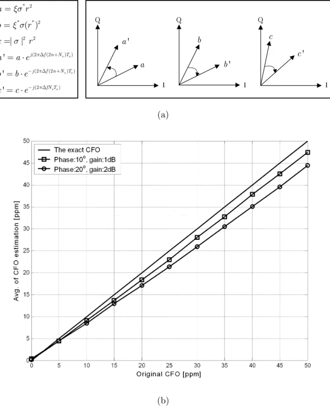
Figure 3-3 (a) Complex plane for the terms in (3.9). (b) CFO estimation by two-repeat preamble-based method under 19 dB SNR... 47
Figure 3-4 Inverse cosine function... 51
Figure 3-5 The flowchart of the proposed P-CFO algorithm... 53
Figure 3-6 Frequency offset estimation... 55
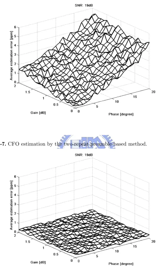
Figure 3-7 CFO estimation by the two-repeat preamble-based method... 56
Figure 3-8 CFO estimation by the proposed P-CFO algorithm... 56
Figure 3-9 PDF of 50 ppm CFO: (a) P-CFO algorithm. (b) Two-repeat preamble-based method... 58
Figure 3-10 Mean square error (MSE) of frequency estimation vs. SNR under different I/Q imbalance conditions with 50 ppm CFO... 59
Figure 3-11 Average of the estimation error... 59
Figure 3-12 Hardware architecture of the P-CFO algorithm... 63
Figure 3-13 Chip micrograph... 64
Figure 3-14 The photo of platform... 65
Figure 3-15 Estimated CFO of measurement vs. simulation... 65
Figure 3-16 Measurements of QPSK constellation: (a) P-CFO method. (b) Two-repeat preamble-based method... 66
Figure 4-1 Direct-conversion receiver with I/Q mismatch and CFO... 72
Figure 4-2 Received signal with I/Q mismatch: (a) Amplitude. (b) Angle... 73
Figure 4-3 The estimated channel frequency response... 76
Figure 4-4 Data flow of the constant IQ-M estimation and compensation... 79
Figure 4-5 (a) The block diagram for the IQ-M estimation. (b) The compensation blocks for IQ-M and CFO... 86
Figure 4-6 Mutual interference due to I/Q mismatch... 88
Figure 4-7 T h e p r o p o s e d f r e q u e n c y - d e p e n d e nt I Q - M e s t i m a t i o n architecture... 90
Figure 4-8 BER performance of 16-QAM and 64-QAM modulation... 92
Figure 4-9 PER performance of 16-QAM and 64-QAM modulation... 93
Figure 4-10 Experiment setup for verification... 94
Figure 4-11 Measurement of constellation diagram: (a) Before compensation. (b) After compensation... 96
Figure 4-14 Block diagram representation of the proposed method. (a) Transmitter part with pre-compensation scheme. (b) Receiver part
with joint compensation scheme... 104
Figure 5-1 Block diagram of the 4 4× STBC MIMO-OFDM modem... 109
Figure 5-2 Space-time block code in the 4 4× MIMO-OFDM system... 111
Figure 5-3 Sub-carrier frequency allocation... 113
Figure 5-4 Block diagram of the adaptive frequency-domain equalizer... 114
Figure 5-5 Relationship between decided symbol and decoded symbol... 116
Figure 5-6 (a) The block diagram of the 2 N× MIMO system. (b) The block diagram of the 3 N× MIMO system with STBC matrix 3 C ... 119
Figure 5-7 BER and PER performance... 123
Figure 5-8 Architecture of the adaptive FD-CE... 124
Figure 5-9 Flowchart of matrix inverse computation... 125
Figure 5-10 Architecture of MI. The bit width includes real and image parts. (a) Matrix multiplier for 1 21,k 11,−k H H and 1 21,k 11,−k 12,k H H H . (b) Matrix multiplier for 1 1 21, 11, k− k −k D H H ... 127
Figure 5-11 Architecture of matrix inverter (Alamouti matrix)... 128
Figure 5-12 Architecture of MM. The bit width includes real and image parts... 129
Figure 5-13 Software-defined radio platform... 131
Figure 5-14 Chip microphotograph of the 4 4× MIMO-OFDM modem... 133
Figure 6-1 A generic digital beamforming system... 136
Figure 6-2 Two-element array for interference suppression... 137
Figure 6-3 (a) Array factor for a non-weighted two-element array. (b) Array factor for a weighted two-element array... 139
Figure 6-4 M-element array with arriving signals... 140
Figure 6-5 M-element array with two arriving signals... 143
Figure 6-6 Capon pseudospectrum... 144
Figure 6-7 MUSIC pseudospectrum... 147
Figure 6-8 Five-element antenna array... 148
Figure 6-9 (a) Array factor for θ =D 0D. (b) Array factor for 30 D θ = D... 151
Figure 6-10 Corresponding array factors. (a) Weight vector = [+1+1]. (b) Weight vector = [+1− ]... 1 152 Figure 6-11 Corresponding array factors. (a) Weight vector = [+1+1+1+1].
[+1−j−1+ ]. (d) Weight vector = [j +1+j −1− ]... 153 j
Figure 6-12 2 2× MIMO WLAN system... 154
Figure 6-13 Channel with angle-time pattern... 155
Figure 6-14 Space-time beamforming architecture... 156
Figure D-1 Transmitter block diagram for IEEE 802.11g (ERP-OFDM only).... 183
Figure D-2 PSDU frame format... 187
Figure D-3 OFDM training structure... 187
Figure D-4 Transmitter block diagram for MIMO-OFDM systems... 189
Figure D-5 (a) The block diagram of the SISO system. (b) The block diagram of the MIMO system with Alamouti scheme... 191
Figure D-6 PSDU frame format... 193
Figure E-1 The radix-2 single-path delay feedback architecture... 195
Figure E-2 Radix-2 SDF butterfly unit... 196
Figure E-3 The processing for IFFT operations... 196
Figure E-4 Frequency offset correction with NCO... 197
Figure E-5 The basic concept of DDFS... 198
List of Acronyms
The following acronyms are used through this text.3G third-generation
3GPP 3rd Generation Partnership Project
ADC analog-to-digital converter AFC auto frequency controller AOA angle-of-arrival
AOD angle-of-departure
API application programming interface APR auto place and routing
AS angular spread
ASIC application-specific integrated circuit AWGN additive white Gaussian noise
BER bit error rate
BPSK binary phase shift keying CFO carrier frequency offset CFR channel frequency response
CMOS complimentary metal-oxide-semiconductor CORDIC coordinate rotation digital computer
CP cyclic prefix
CRLB Cramér-Rao lower bound CSI channel state information DA data-aided
DAB digital audio broadcasting DAC digital-to-analog converter DC direct current
DOA direction of arrival DRC design rule checking
EVM error vector magnitude
FD-CE frequency-domain channel estimator FEC forward error correction
FFT fast Fourier transform FPGA field programmable gate array GI guard interval
GIB guard interval based
HDL hardware-description language ICI inter-carrier interference IFFT inverse fast Fourier transform I/Q in phase/quadrature phase IQ-M I/Q mismatch
IRR image rejection ratio LO local oscillator LPF low-pass filter LSB least significant bit LTE long term evolution LVS layout versus schematic MAC medium access control MAN metropolitan area network MG mirror gain
MI matrix inverter MIMO multi-input multi-output MISO multiple-input single-output ML maximum likelihood MM matrix multiplier
MMSE minimum mean square error MSE mean square error MUSIC multiple signal classification NCO numerically controlled oscillator NDA non-data-aided
NLS nonlinear least squares
OFDM orthogonal frequency-division multiplexing OFDMA orthogonal frequency-division multiple access P-CFO pseudo carrier frequency offset
PDA personal digital assistant PDF probability density function
PER packet error rate PHY physical layer
PLCP physical layer convergence procedure PPDU PLCP protocol data unit
PSDU physical layer service data unit QAM quadrature amplitude modulation QPSK quadrature phase shift keying R2SDF radix-2 single-path delay feedback RF radio frequency
RMS root mean square RX receiver
SC-FDMA single carrier-frequency division multiple access SDM spatial-division multiplexing
SG signal gain
SIMO single-input multiple-output SIR signal-to-interference ratio SISO single-input single-output SNR signal-to-noise ratio
SQNR signal-to-quantization noise ratio STBC space-time block code
TX transmitter
UMTS universal mobile telecommunication system VANET vehicular ad hoc network
VHT very high throughput
VLSI very-large-scale integration WLAN wireless local area network ZF zero-forcing
Chapter 1
Introduction
1.1 Motivation
In recent years, there is an increasing application for higher spectrum efficient, higher data rate, better quality of service, and higher system capacity. The data rate and mobility of some wireless communication standards are shown in Figure 1-1. There is a trend that multi-input multi-output (MIMO) transmission has emerged as a potential technology in the future standards. Specifically, MIMO techniques have been integrated into third-generation (3G) cellular systems [1], wireless local area networks (IEEE 802.11n) [2], and broadband wireless access networks (IEEE 802.16e) also known as WiMAX [3]. MIMO communication systems are defined by considering that multiple antennas are used at the transmit part as well as at the receive part. By using the spatial and polarization properties of the multipath channels, MIMO communication systems offer new dimensions that can be used to enhance the quality of communication.
Range (km)
Figure 1-1. Data rate versus mobility of wireless communication standards.
Due to the use of antenna arrays, spatial diversity can be obtained. The concept of spatial diversity is that the signal-to-noise ratio is significantly improved by combining the signal transmitted from different antennas. In order to approach the capacity of MIMO channels, the space-time processing is employed. Space-time processing is a tool for improving the overall economy and efficiency of a MIMO communication system. Space-time processing can improve the signal-to-interference ratio through co-channel interference cancellation, mitigate fading through receive diversity, offer higher signal-to-noise ratio through array gain, and reduce inter-symbol interference through spatial equalization.
In addition, orthogonal-frequency division multiplexing (OFDM) is a popular technique which operates with specific orthogonality constraints between sub-carriers. Because of these constraints, OFDM modulation is a spectrally efficient signaling
method for communication over frequency-selective fading channels. OFDM modulation has been utilized by many standards, including IEEE 802.11a/g/n-based WLAN systems [2], [4], [5], digital audio broadcasting (DAB) [6], and digital video broadcasting terrestrial TV (DVB-T) [7]. Therefore, MIMO-OFDM arrangements have been suggested for frequency-selective fading channels, where space-time coding or space-frequency coding is used across the different antennas in conjunction with OFDM [8].
In this study, a 4 4× MIMO-OFDM communication system and advanced receiving techniques are explored. The transceiver design and implementation are also presented. In order to realize the 4 4× MIMO-OFDM communication system, some impairments are taken into account. For instance, synchronization tasks, such as timing synchronization and frequency synchronization, are essential in the practical implementation. Other impairments which can degrade the system performance are channel effects and non-ideal front-ends. To support reliable reception of the transmitted data, robust algorithms must be developed.
A software-defined radio is also constructed for rapid verification and fast prototyping. This experimental platform comprises of MATLAB model, field programmable gate array (FPGA) board, and radio frequency (RF) front-end. The proposed design is directly mapped onto the FPGA chips with on-board 14-bit digital-to-analog converters (DACs) to transform the digital data into analog signals. The signals are then transmitted by RF front-ends. After down-converting RF signals to baseband at receiver part, the analog signals are fed into 14-bit analog-to-digital converters (ADCs).
Another important issue is the implementation cost. In order to achieve low hardware cost and low power consumption, low complexity algorithms and efficient very-large-scale integration (VLSI) architectures are preferable. For instance, the
proposed algorithms are evaluated using additional factors, such as numerical precision, relative VLSI architecture, and memory requirements. Based on the overall system performance index, the implementation trade-offs can be balanced.
1.2 Dissertation
Overview
The system considerations and channel models are introduced in Chapter 2. A brief introduction of the MIMO-OFDM system is given. The fundamental understanding of MIMO technology and space-time processing is presented. In addition, the impact of impairments on the system performance is also discussed. In order to maintain the system performance, some essential algorithms are developed.
In Chapter 3, an anti-I/Q mismatch (IQ-M) auto frequency controller (AFC) is developed. Frequency synchronization is a critical problem for the MIMO-OFDM system. Various frequency offset estimation algorithms have been developed in the open literature. However, it is shown that some methods are not suitable for current wireless systems since the packet format is not compatible with current standards. The proposed carrier frequency offset (CFO) estimation method, based on pseudo CFO (P-CFO) technology, can estimate the CFO value under the conditions of IQ-M. Additionally, the proposed P-CFO algorithm is also compatible with the conventional method.
In Chapter 4, preamble-assisted estimation methods are developed to circumvent the effect of IQ-M. Because IQ-M can degrade the accuracy of CFO estimation and introduce image interference, the compensation for IQ-M is necessary. Many IQ-M estimation methods are published in the open literature. However, most methods focus on the constant IQ-M only. Because of the impairment in the analog components, the low-pass filters of I and Q channels are not identical, resulting in frequency-dependent
IQ-M. The proposed methods can estimate not only constant IQ-M but also frequency-dependent IQ-M.
In Chapter 5, an adaptive channel estimator in STBC MIMO-OFDM modems is developed. In order to realize the gains obtained from MIMO cannels, obtaining accurate channel state information in time-varying environments is extremely important. In order to reduce the hardware cost, the proposed adaptive channel estimator utilizes the property of the Alamouti-like matrix to decrease the cost of complex operators.
In Chapter 6, digital beamforming for wireless communications is presented. In order to improve the signal quality, digital beamforming is performed digitally to form the desired output.
Finally, Chapter 7 describes the conclusions of this work and indicates some promising directions for future research.
Chapter 2
Overview of MIMO-OFDM Systems
This chapter serves as a brief introduction to multi-input multi-output (MIMO) orthogonal frequency-division multiplexing (OFDM) wireless communication systems. The impact of non-ideal front-ends on system performance is also discussed.
2.1 MIMO Wireless Communications
2.1.1 Antenna Configurations
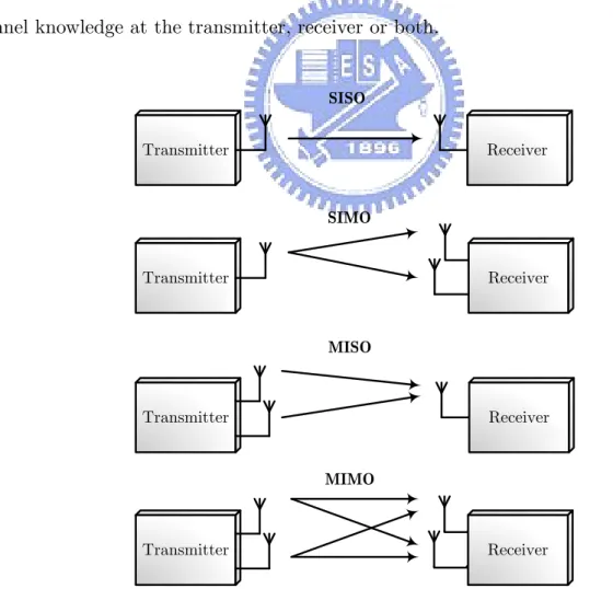
Figure 2-1 shows different antenna configurations. Single-input single-output (SISO) which uses one transmit antenna and one receive antenna is the well-known configuration, single-input multiple-output (SIMO) uses one transmit antenna and multiple receive antennas, multiple-input single-output (MISO) has multiple transmit antennas and a single receive antenna, and, finally, MIMO has multiple transmit
antennas and multiple receive antennas.
With MIMO, the system can effectively provide the array gain [9]-[12]. Array gain is the average increase in the signal-to-noise ratio (SNR) at the receiver that arises from the coherent combining effect of multiple antennas at the receiver, transmitter or both. If the channel is known to the multiple antenna transmitter, the transmitter can weight the transmission with weights, depending on the channel state information, so that there is coherent combining at the single antenna receiver. The array gain in this case is called transmitter array gain. For the SIMO system with perfect knowledge of the channel at the receiver part, the receiver can suitably weight the incoming signals so that the signals are coherently added up at the output. This case is called receiver array gain. In order to achieve the array gain, multiple antenna systems require perfect channel knowledge at the transmitter, receiver or both.
SISO SIMO MISO MIMO Transmitter Transmitter Receiver Receiver Receiver Receiver Transmitter Transmitter
2.1.2 Capacity Results
Based on Shannon’s theorem, capacity is a measure of the maximum transmission rate for reliable communication on a given channel. Firstly, let us consider the SISO system on the additive white Gaussian noise (AWGN) channel. The capacity of the channel is expressed as
( )
2
log 1 (bits/s/Hz)
C = +P (2.1)
where P is the average signal-to-noise ratio (SNR) at the receiver. The capacity, as
defined in (2.1), is also known as the spectral efficiency. If the transmission rate is less than C bits/s/Hz, then an appropriate coding scheme exists that could lead to reliable
and error-free communication. On the contrary, if the transmission rate is more than C
bits/s/Hz, then the received signal, regardless of the employed coding scheme, will involve bit errors. MIMO communication technology has received significant attention due to the rapid development of high-speed wireless communication systems employing multiple transmit and receive antennas. Theoretical results show that MIMO systems can offer significant capacity gain over traditional SISO channels. This increase in capacity is enabled by the fact that in rich scattering environments, the signals from each transmitter appear highly uncorrelated at each of the receive antennas, i.e., the signals corresponding to each of the individual transmit antennas have attained different spatial signatures. The receiver exploits these differences in spatial signatures to separate these signals.
MIMO Transmitter h11 h12 h1,M MIMO Receiver 1 2 M 1 2 N
Figure 2-2. Block diagram of the MIMO system.
Figure 2-2 shows the block diagram of the MIMO system with M transmit
antennas and N receive antennas. The input-output relationship of this system is expressed as = + Y HX W (2.2) where [ 1 2 ... ]T M x x x =
X is the transmitted data vector, [ 1 2 ... ]T N
y y y
=
Y
is the received data vector, and [ 1 2 ... ]T N
w w w
=
W is the noise vector. H
denotes the N×M channel matrix which is defined by
11 12 1, 21 22 2, ,1 ,2 , M M N N N M h h h h h h h h h ⎡ ⎤ ⎢ ⎥ ⎢ ⎥ ⎢ ⎥ = ⎢ ⎥ ⎢ ⎥ ⎢ ⎥ ⎢ ⎥ ⎢ ⎥ ⎣ ⎦ H " " # # % # " (2.3)
where h is the complex gain from the jth transmit antenna to the ith receiver antenna. ij
channel is given by [13]
2
log det P H (bits/s/Hz)
C
M
⎛ ⎛ ⎞⎟⎞
⎜ ⎜ ⎟
= ⎜⎜⎝ ⎜⎜⎝I+ HH ⎟⎟⎠⎟⎠⎟ (2.4)
where I denotes the identity matrix, the superscript H indicates the conjugate transpose, and P is the per-receive antenna SNR. In order to gain insight on the
capacity, (2.4) can be expressed as [13]
min{ , } 2 1 log 1 (bits/s/Hz) N M i i P C M λ = ⎛ ⎞⎟ ⎜ = ⎜⎜⎝ + ⎟⎟ ⎠
∑
(2.5)where λ denotes the eigenvalues of the rectangular i HH matrix. Mainly, the H
capacity is equal to the richness of the channel plus a term depending on the power level.
2.1.3 Space-Time Processing
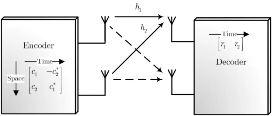
In order to improve the reliability for MIMO communication, space-time coding techniques are developed. A pioneering work in the area of space-time coding for MIMO channels has been carried out by Tarokh et al. in [14]-[15]. However, the coding scheme in [14]-[15] requires high decoding complexity. Afterward, Alamouti developed the most famous space-time block coding (STBC) scheme for two transmit and multiple receive antennas [16]. The complexity of the maximum likelihood decoder for Alamouti’s code is very low. Figure 2-3 shows the block diagram of the 2 2× MIMO system with Alamouti’s code. The encoding rule of Alamouti’s scheme is
1 h 2 h 1 2 r r ⎡ ⎤ ⎢ ⎥ ⎣ ⎦ 1 2 2 1 c c c c ∗ ∗ ⎡ − ⎤ ⎢ ⎥ ⎢ ⎥ ⎢ ⎥ ⎣ ⎦
Figure 2-3. Block diagram of the 2 2× MIMO system with Alamouti’s scheme.
1 2 1 2 2 1 c c c c c c ∗ ∗ ⎡ − ⎤ ⎢ ⎥ ⎡ ⎤ → ⎢ ⎥ ⎢ ⎥ ⎣ ⎦ ⎢ ⎥ ⎣ ⎦ (2.6)
where , 1,2c i =i terms represent the transmitted complex symbols. In the first time slot, antenna one transmits c and antenna two transmits 1 c . In the next time slot, 2
antenna one transmits −c2∗ and antenna two transmits c1∗. The columns of the matrix represent time slots and the rows denote transmit antennas. Since two time slots are required to transmit two symbols, the code rate for Alamouti’s scheme is equal to one. Assuming that the channel coefficients are constant in both consecutive symbol periods, the symbols received by antenna one over two consecutive time slots are given by
1 1 2 1 1 2 2 2 1 2 r h h x w x r∗ h∗ h∗ w∗ ⎡ ⎤ ⎡ ⎤ ⎢ ⎥⎡ ⎤ ⎡ ⎤ ⎢ ⎥ = ⎢ ⎥⎢ ⎥+⎢ ⎥ ⎢ ⎥ − ⎢ ⎥ ⎢ ⎥ ⎢ ⎥ ⎢ ⎥⎣ ⎦ ⎢ ⎥ ⎣ ⎦ ⎣ ⎦ ⎣ ⎦ (2.7)
Assuming that the receiver has knowledge of the channel coefficients, the decision statistics are given by
(
)
1 1 2 1 1 1 2 2 1 2 2 2 2 1 ˆ ˆ r h h x h h r x h h − − ∗ ∗ ∗ ⎡ ⎤ ⎡ ⎤ ⎢ ⎥ ⎡ ⎤ ⎢ ⎥ = + ⎢ ⎥ ⎢ ⎥ ⎢ ⎥ ⎢ − ⎥ ⎢ ⎥⎢ ⎥ ⎢ ⎥ ⎣ ⎦ ⎣ ⎦ ⎣ ⎦ (2.8)Adding all the decision statistics from all N receive antennas, the estimated symbols will be a scale version. In order to estimate the symbols, we can scale the decision statistics. This result presented above can be directly extended to other STBC codes.
1,1 1,64 x x ⎡ ⎤ ⎢ ⎥ ⎢ ⎥ ⎢ ⎥ ⎢ ⎥ ⎢ ⎥ ⎣ ⎦ # 2,1 2,64 x x ⎡ ⎤ ⎢ ⎥ ⎢ ⎥ ⎢ ⎥ ⎢ ⎥ ⎢ ⎥ ⎣ ⎦ # 2,1 2,64 x x ∗ ∗ ⎡− ⎤ ⎢ ⎥ ⎢ ⎥ ⎢ ⎥ ⎢ ⎥ ⎢− ⎥ ⎢ ⎥ ⎣ ⎦ # 1,1 1,64 r r ⎡ ⎤ ⎢ ⎥ ⎢ ⎥ ⎢ ⎥ ⎢ ⎥ ⎢ ⎥ ⎣ ⎦ # 2,1 2,64 r r ⎡ ⎤ ⎢ ⎥ ⎢ ⎥ ⎢ ⎥ ⎢ ⎥ ⎢ ⎥ ⎣ ⎦ # 1,1 1,64 x x ∗ ∗ ⎡ ⎤ ⎢ ⎥ ⎢ ⎥ ⎢ ⎥ ⎢ ⎥ ⎢ ⎥ ⎢ ⎥ ⎣ ⎦ # 1 h 2 h
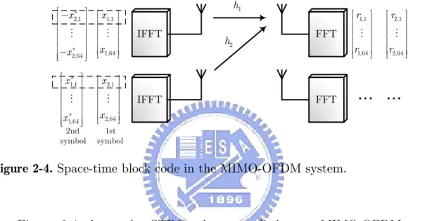
Figure 2-4. Space-time block code in the MIMO-OFDM system.
Figure 2-4 shows the STBC scheme applied to a MIMO-OFDM system. In MIMO-OFDM systems, STBC is used independently to each sub-carrier [17]. For the convenience of explanation, two transmit antennas and one receive antenna are considered. Let r denote the kth received sub-carrier at the ith symbol duration. The i k,
received data over two consecutive symbol periods at receiver one are expressed as
1, 1, 1, 2, 2, 1, 2, 1, 2, 2, 1, 2, k k k k k k k k k k k k r h x h x w r h x∗ h x∗ w = + + = − + + (2.9)
where h is the channel frequency response for the kth sub-carrier from the ith i k,
transmit antenna to the receiver and w is the noise term. The received data are then i k,
1, 1, 2, 1, 1, 2, 2, 2, 1, 2, k k k k k k k k k k k k k k r h h x w x r∗ h∗ h∗ w∗ ⎡ ⎤ ⎡ ⎤ ⎢ ⎥⎡ ⎤ ⎡ ⎤ ⎢ ⎥ =⎢ ⎥⎢ ⎥+⎢ ⎥ ⎢ ⎥ − ⎢ ⎥ ⎢ ⎥ ⎢ ⎥ ⎢ ⎥⎣ ⎦ ⎢ ⎥ ⎣ ⎦ ⎣ ⎦ ⎣ ⎦ ⇒R = H X +W (2.10)
where R , k X , and k W are 2 1k × vectors and H is a 2 2k × matrix. The received symbols can be decoded by the STBC decoder with the estimated channel state information (CSI). The data are then equalized by the following equation.
1 ˆk = k− k
X H R (2.11)
In contract with STBC scheme, spatial-division multiplexing (SDM) technique is used to achieve higher throughput [18]. With SDM, multiple transmit antennas transmit independent data streams, which can be individually recovered in the receiver. An applicable method is required to separate each transmitted stream form other transmitted streams (interference cancellation). Many approaches, such as zero-forcing (ZF), minimum mean square error (MMSE), and maximum likelihood (ML) detectors, are known for the detection of SDM signals. However, the computation complexity of performing a full search for ML detection is too high to be suitable for practical applications. In order to reduce the complexity, various MIMO detection methods, such as sphere decoding technique [19] or K-best algorithm [20], have been proposed. Different detection methods have different criteria, and therefore it is preferred to adopt a reduced-complexity data detection scheme for MIMO systems.
2.1.4 MIMO-OFDM Systems
OFDM has been shown to be an effective technique to combat multipath fading in wireless channels [21]-[23]. It has been used in various wireless communication systems such as wireless local area network (WLAN) and wireless metropolitan area network (WMAN). OFDM is a multi-carrier technique that operates with specific orthogonality constraints between the sub-carrier. OFDM is attractive since it admits relatively easy solutions to some difficult challenges that are encountered when using single-carrier modulation schemes on wireless channels. Due to the demand for high speed wireless applications and limited radio frequency (RF) signal bandwidth, OFDM is being considered in the standard that considers MIMO systems, where multiple antennas are used for the purpose of spatial multiplexing or to provide increased spatial diversity.
Figure 2-5 displays the block diagram of the 4 4× MIMO-OFDM system. In the MIMO-OFDM system, the incoming bit stream is first encoded by the one-dimensional encoder (FEC encoder), and then the encoded bits are mapped onto three dimensions (time, frequency, and space) by the space-time coding. The receiver uses the preambles to complete the synchronization, and transforms the signal from time to frequency domain. Spatial streams are then demodulated to bit-level streams, which are de-interleaved and merged into a data stream. Finally, the data stream is decoded by the forward error correction decoder.
Although OFDM is robust against the multi-path propagation, it is very sensitive to the non-ideal front-end effects that destroy the orthogonality between sub-carriers. For example, OFDM is vulnerable to non-linearity, timing offset and frequency offset [21]. Hence, MIMO-OFDM systems also inherit these disadvantages of the OFDM modulation. In the following section, the non-ideal front-end effects will be discussed.
.. . ... ... .. . ... .. . ... .. . ... ... ... ... ... .. . ... ... .. . ... .. . ... ... ... ... ... ... ...
Figure 2-5. Block diagram of the 4 4× MIMO-OFDM system.
2.2 Non-Ideal Front-End Effects
The receiver architecture adopted in this work is based on the direct-conversion architecture. A block diagram of the direct-conversion receiver is shown in Figure 2-6. The direct-conversion receiver converts the carrier of the desired channel to the zero frequency immediately in the first mixers [24]-[26]. Hence, the direct-conversion is often called also as a zero-intermediate frequency (IF) receiver. Since the direct-conversion receiver has no IF, the evident benefit of the this architecture is low hardware cost. However, the direct-conversion receivers are sensitive to several non-ideal effects caused in the front-end. These non-idealities will be covered in the following subsections.
In this work, the MIMO-OFDM system shares the local oscillator (LO) and the sampling clock. In this way, the synchronization error is common to all receive branches, resulting in a simplified implementation.
Baseband ADC ADC 90D LNA VGA VGA Low-pass Filter Low-pass Filter Mixer Mixer I Q Sampling Clock Local Oscillator Figure 2-6. Direct-conversion receiver.
2.2.1 Effects of Carrier Frequency Offset
Basically, the band-pass signal yRF( )t at carrier frequency f can be expressed as c
{
}
{
}
(
)
{
}
(
)
2 2 2 ( ) Re ( ) Re ( ) cos 2 Im ( ) sin 2 1 ( ) ( ) 2 c c c f t RF c c f t f t y t r t e r t f t r t f t r t e r t e π π π π π ∗ − = = − ⎡ ⎤ = ⎢⎣ + ⎥⎦ (2.12)where ( )r t is the complex baseband signal and the initial phase of the carrier is
neglected. Re ( )
{
r t}
and Im ( ){
r t}
denote the in-phase component and the quadrature component of ( )r t , respectively. Based on the direct-conversion receiver,( ) 2 2 2 2 2 2 ( ) 2 ( ) ( ) ( ) ( ) c c c c c f t f t f t f t RF f t y t e r t e r t e e r t r t e π π π π π − ∗ − − − ∗ ⎡ ⎤ ⋅ = ⎢⎣ + ⎥⎦ = + (2.13) cos(2πf tc ) sin(2πf tc ) − ( ) RF y t
{
}
Re ( )r t{
}
Im ( )r t j × ( ) r t (a) f 0 2fc 2fc − |R fI( )| f 2fc 2fc − |R fQ( )| f |YRF( )|f c f 0 c f − f | ( )|Rf 0 j × cos(2πf tc) −sin(2πf tc) 2 2 cos(2 ) 2 j ft j ft e e ft π π π = + − sin(2 ) 2 2 2 j ft j ft e e ft j π π π = − − (b)Figure 2-7. (a) I/Q demodulation. (b) Signal spectrum.
After passing through the low-pass filters (LPFs), the complex baseband signal ( )r t is
regenerated. The process (I/Q demodulation) in the spectrum domain is shown in Figure 2-7.
In practice, OFDM is sensitive to carrier frequency offset (CFO) due to the mismatch of LOs between the transmitter and the receiver. The presence of CFO introduces inter-carrier interference (ICI), which can degrade the system performance significantly. When the system suffers from CFO fΔ , the received signal after baseband processing is given by [27]
{
}
{
}
{
}
{
}
{
}
2
( ) ( ) ( )
cos(2 )Re ( ) sin(2 ) Im ( )
sin(2 )Re ( ) cos(2 ) Im ( )
( ) j ft y t r t e w t ft r t ft r t j ft r t ft r t w t π π π π π Δ = + = Δ − Δ + Δ + Δ + (2.14)
where ( )w t denotes the representations of the additive white Gaussian noise (AWGN).
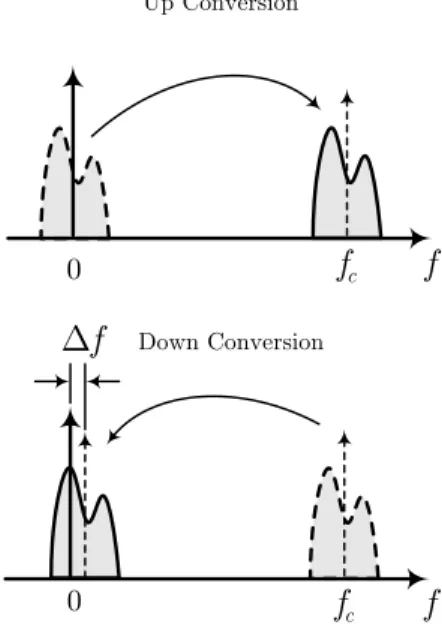
From (2.14), the CFO effect results in phase shift in the time domain. The behavior of CFO in the spectrum domain is shown in Figure 2-8. It is clear that the spectrum is shifted with a frequency Δ . After digitizing the signal and passing through the FFT f
block, the frequency domain data is given by (see Appendix A for details) [28]
f c f 0 Up Conversion f c f 0 f Δ Down Conversion
{
}
( )(
)
( ) ( )(
)
( 1)/ ( 1)/ ( )/ , FFT ( ) sin sin sin sin k N j N N k k K j N N j l k N l l k k K l k Y y n X H e N N X H e e W N l k N πε πε π πε πε πε π ε − − − − =− ≠ = ⎧ ⎫ ⎪ ⎪ ⎪ ⎪ ⎪ ⎪ = ⎨⎪ ⎬⎪ ⎪ ⎪ ⎪ ⎪ ⎩ ⎭ ⎧ ⎫ ⎪ ⎪ ⎪ ⎪ ⎪ ⎪ + ⎨⎪ ⎬⎪ + − + ⎪ ⎪ ⎪ ⎪ ⎩ ⎭∑
(2.15)where the subscript N denotes the FFT size. X and k H denote the data carrier and k
channel frequency response, respectively. The frequency offset fΔ is normalized to sub-channel bandwidth, and the relative frequency offset is shown as ε . In (2.15), the
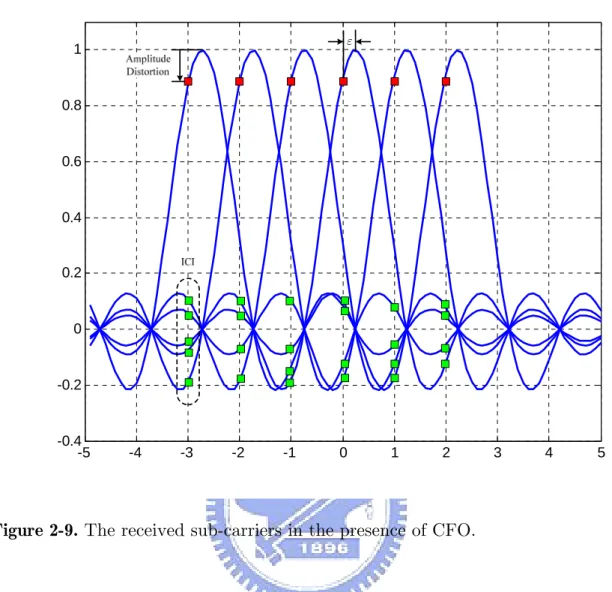
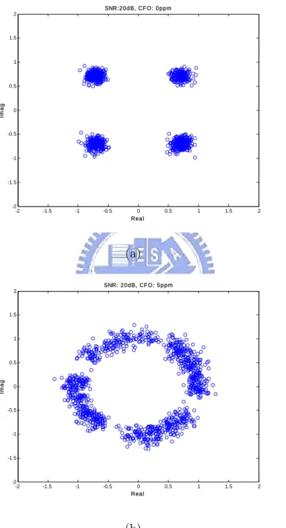
first term of the right hand side is the decayed original signal transmitted in the kth sub-carrier, and the second term denotes the inter-carrier interference (ICI) from others. All sub-carriers in an OFDM symbol are orthogonal if they all have a different integer number of cycles within the FFT interval. If there is CFO, the number of cycles in the FFT interval will not be an integer. When the LOs between the transmitter and the receiver are not aligned, CFO occurs and the frequency spectrum is not sampled at the optimum peaks of the sinc functions. The property is shown in Figure 2-9. In Figure 2-9, the received data on each sub-carrier is not the original transmitted data when there is CFO. The effect of frequency offset on a QPSK constellation is depicted in Figure 2-10. With 5 ppm CFO value, the constellation points have rotated over the decision boundaries after 10 OFDM symbols. Since the phase rotation is increasing with time, it has to be compensated even for a small CFO.
-5 -4 -3 -2 -1 0 1 2 3 4 5 -0.4 -0.2 0 0.2 0.4 0.6 0.8 1 ε
Figure 2-9. The received sub-carriers in the presence of CFO.
Another reason causing CFO is the Doppler shift of the RF carrier. As the result of the relative motion between the transmitter and the receiver, each multipath wave is subject to a frequency shift. The frequency shift of the received signal caused by the relative motion is called the Doppler shift, which is proportional to the speed of the mobile unit. When a signal with carrier frequency f is transmitted and the received c
signal comes at an incident angle θ with respect to the direction of the vehicle motion, the Doppler shift f of the received signal is given by [29] D
cos( ) D v f c θ = (2.16)
practical conditions, the Doppler effect adds some hundreds of Hz in frequency spreading. -2 -1.5 -1 -0.5 0 0.5 1 1.5 2 -2 -1.5 -1 -0.5 0 0.5 1 1.5 2 Rea l Im a g SNR:2 0d B, CF O: 0 pp m (a) -2 -1.5 -1 -0.5 0 0.5 1 1.5 2 -2 -1.5 -1 -0.5 0 0.5 1 1.5 2 Rea l Im ag SNR: 20 dB, CF O : 5p p m (b)
Figure 2-10. QPSK constellation in the case of the AWGN channel. (a) CFO: 0 ppm.
2.2.2 Effects of I/Q Mismatch
cos(2πf tc )( )
RFy
t
1+ε 90D +ϕ( )
y n
Figure 2-11. Direct-conversion receiver with I/Q mismatch.Figure 2-11 depicts the block diagram of a direct-conversion architecture. I/Q mismatch (IQ-M) arises when the phase and gain differences between I and Q branches are not exactly 90 degree and 0 dB, respectively [26]. The mismatched LO output signals are modeled as : cos(2 ) : (1 )sin(2 ) c c I f t Q f t π ε π ϕ − + + (2.17)
where ε and ϕ denote the constant amplitude and phase mismatch, respectively. Multiplying the band-pass signal by the mismatched LO signals and passing through the LPFs, the baseband signal is expressed as [30]-[31]
{
}
{
}
{
}
( )(
)
(
( ))
( ) Re ( ) (1 ) Im ( ) cos Re ( ) sin ( ) 0.5 1 1 ( ) 0.5 1 1 ( ) ( ) ( ) ( ) ( ) j j y n r n j r n r n w n e r n e r n w n r n r n w n ϕ ϕ ε ϕ ϕ ε ε α β − ∗ ∗ ⎡ ⎤ = + + ⎣ − ⎦+ = + + + − + + = + + (2.18)the OFDM system, the received signal is further passed through the FFT block. After the FFT operation, the frequency-domain data can be expressed as
{
}
FFT ( ) k N k k k k k k k k Y y n R R W H X H X W α β α β ∗ − ∗ ∗ − − = = + + = + + (2.19)Equation (2.19) shows that IQ-M can cause the symbol at the sub-carrier k to be scaled by the complex factor α . Moreover, the complex conjugate of the symbol at sub-carrier –k multiplied by another complex factor β will be present. The desired sub-carrier k will include the unwanted interference related to the sub-carrier –k, implying that IQ-M can distort the accuracy of received signal. The effect of IQ-M on the 16-QAM constellation is depicted in Figure 2-12. As a result of the IQ-M, the constellation is distorted severely. It implies that IQ-M can limit the ability of the receiver to achieve better performance especially for high constellation size, e.g., 64-QAM constellation.
The image reject ratio (IRR) as a function of the mismatch is given by [32]
2 2 1 (1 ) 2(1 )cos( ) IRR 10 log (dB) 1 (1 ) 2(1 )cos( ) ε ε ϕ ε ε ϕ ⎡ + + + + ⎤ ⎢ ⎥ = ⋅ ⎢ ⎥ + + − + ⎣ ⎦ (2.20)
A plot of (2.20) is shown in Figure 2-13. In order to achieve an IRR of at least of 55 dB, the gain error must be smaller than 0.3% and the phase error must be smaller than 0.1 degree. Another design choice is that the gain error must be smaller than 0.1% and the phase error must be smaller than 0.2 degree.
(a)
(b)
Figure 2-12. 16-QAM constellation. (a) Without I/Q mismatch. (b) Gain error: 1dB,
0 0.05 0.1 0.15 0.2 0.25 0.3 0.35 0.4 0.45 0.5 25 30 35 40 45 50 55 60 65 70
Phase error (deg.)
IR R ( d B ) gain error:10% gain error: 1% gain error: 0.3% gain error: 0.1% 0.3%, 0.1 deg. 0.1%, 0.2 deg.
Figure 2-13. Image suppression as a function of the I/Q mismatch.
This mismatch can occur at the transmitter, receiver or both. Moreover, due to the impairment in the analog components, the low-pass filters (LPFs) of I and Q channels are not identical. The mismatched LPFs result in frequency-dependent IQ-M. Frequency-dependent IQ-M means that the imbalances can vary with frequency. This will be further discussed in Chapter 4.
2.2.3 Effects of Non-linearity
The power transfer function of a power amplifier is shown in Figure 2-14. In Figure 2-14, the 1 dB compression point is labeled as P1dB and is defined as the point at which a 1 dB increase in input power results in 1 dB decrease in the linear gain of the amplifier [26]. For low values of the input power, the output power grows approximately linear. For intermediate values, the output power falls below that linear growth and it runs into a saturation as the input power grows higher. The dynamic range of amplifier, which also corresponds to the linear region of operation for an amplifier, is defined between the noise-limited region and the saturation region. In order to recognize the signal, saturation should be avoided as much as possible.
1 dB in P out P Nonlinear amplifier 1dB P
Figure 2-14. Power transfer function.
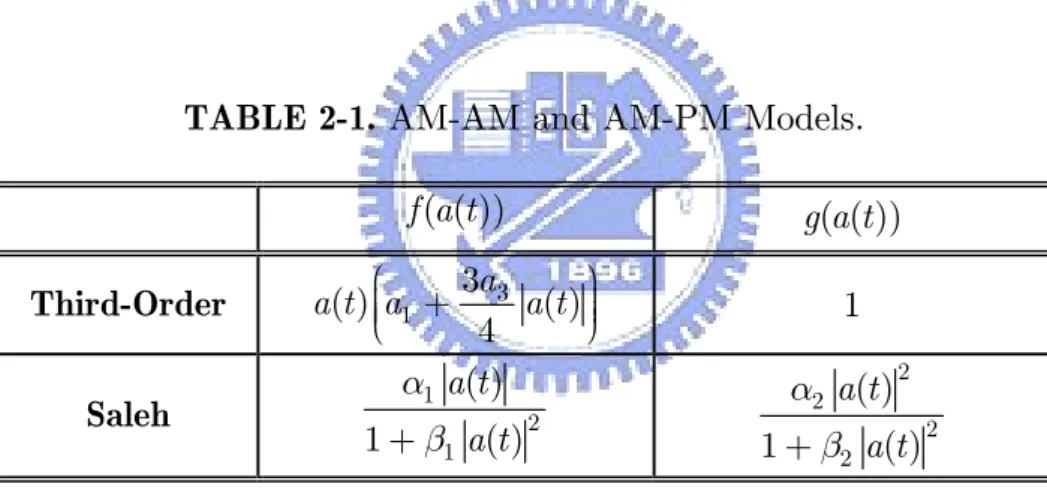
The actual saturation behavior is difficult to model. Common AM-AM (amplitude modulation/amplitude modulation) and AM-PM (amplitude modulation/phase modulation) models are the third-order model and the Saleh model [33]. These mathematical models are listed in TABLE 2-1. In TABLE 2-1, coefficients a , i α and i
Considering an OFDM complex baseband signal x t( )=a t e( ) j tφ( ) with amplitude ( )a t and phase ( )φ that passes a non-linear amplifier, the output is expressed as t
( ( ( )) ( )) ( ) ( ( )) j g a t t
y t = f a t e +φ (2.21)
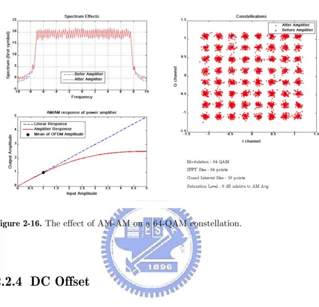
where ( ( ))f a t and ( ( ))g a t describe the AM-AM and AM-PM characteristics, respectively. An example of distortion on a 64-QAM constellation due to AM-AM is displayed in Figure 2-16. In addition, non-linearity can cause spectral widening of the transmit signal resulting in unwanted out-of-band noise. At the transmitter part, the transmitted signal itself is degraded by nonlinearities, resulting in increased bit error rates in the receiver.
TABLE 2-1. AM-AM and AM-PM Models.
( ( )) f a t g a t ( ( )) Third-Order 3 1 3 ( ) ( ) 4 a a t a⎛⎜ +⎜⎜⎝ a t ⎞⎟⎟⎟⎠ 1 Saleh 1 2 1 ( ) 1 ( ) a t a t α β + 2 2 2 2 ( ) 1 ( ) a t a t α β + ( ) x t amplitude ( ) y t phase
Figure 2-16. The effect of AM-AM on a 64-QAM constellation.
2.2.4 DC Offset
Another important source for reduction of the dynamic range in the analog part is direct current (DC) offset. Static DC offset may be generated by bias mismatch in the baseband chain, but also generated from self-mixing of the RF signal with the LO due to imperfect LO–RF isolation on the same substrate [24]-[26]. In addition, dynamic DC offset can be introduced by mixing of close-in interference with the LO signal. In general, the OFDM system uses null DC. The reason is that the DC offset can be removed by applying a DC blocking filter since there is no information around DC.
2.2.5 Quantization Noise and Clipping
In order to reduce the cost and power consumption, the number of bits of the analog-to-digital converter (ADC) and digital-to-analog converter (DAC) must be kept as low as possible [27], [34]. On the other hand, it is desirable to have a large number of bits to reduce the quantization noise. Assuming the input analog voltage range is from − Vp
to + volt and the ADC has N bit output words, the least significant bit (LSB) Vp
value is 1 2 2 2 p p LSB N N V V A = = − (2.22)
Assuming a linear conversion slope, the amplitude error is comprised between −ALSB 2
and +ALSB 2. If the quantization error v is uniform over [−ALSB 2,+ALSB 2], the variance of the quantization error is
/ 2 / 2 2 2 2 12 LSB LSB A LSB A A v dv σ + − =
∫
= (2.23)Replacing ALSB in (2.23) with ALSB =2Vp 2N , (2.23) can be written as
( )
( )
2 2 2 2 2 2 3 2 12 2 p p N N V V σ = = ⋅ ⋅ (2.24)If the signal input is a full-scale sinusoidal signal, the signal-to-quantization noise ratio (SQNR) is
[
]
ADC 10 2 10 2 2 2 2 10 2 10 10 input signal SQNR 10 log quantization noise 2 10 log 12 2 2 10 log 12 10 log (6) (2 2) log (2) 6.02 1.76 (dB) p LSB N LSB LSB A A A A N N − ⎛ ⎞⎟ ⎜ = ⎜⎜ ⎟⎟⎟ ⎝ ⎠ ⎛ ⎞⎟ ⎜ ⎟ ⎜ = ⎜⎜ ⎟⎟ ⎟⎟ ⎜⎝ ⎠ ⎛ ⎞⎟ ⎜ ⎟ ⎜ = ⎜⎜ ⎟⎟ ⎟⎟ ⎜⎝ ⎠ = + − ⋅ = + (2.25)From (2.25), it is clear that quantization in the ADC sampling process introduces noise. In the receiver chain, the received signal is adjusted to make the signal fit in the ADC dynamic range. If the signal is strongly amplified, the signal peaks can be clipped, resulting in severe distortion. Figure 2-17 shows the effects of quantization noise and clipping. During implementation, there is a trade-off between quantization noise and clipping. 0 1 2 3 4 5 6 7 8 9 10 -1 -0.8 -0.6 -0.4 -0.2 0 0.2 0.4 0.6 0.8 1 Original 8-level 16-level
2.3 Wireless
Channel
Models
In communication system design, communication channel plays an important role since the transmitter and receiver designs have to be optimized with respect to the target channel. Without loss of generality, we discuss the channel characterization based on the SISO system. Some frequently used statistical models are reviewed in the following subsections.
2.3.1 AWGN
In the baseband, electronic and thermal noises are generally combined and modeled as an additive white Gaussian noise (AWGN) with zero mean and standard deviation σ . The Gaussian distribution is defined as
( )2 2 2 1 ( ) 2 x p x e μ σ σ π − − = (2.26)
where μ is the mean and σ denotes the variance. When modeling AWGN in the 2 phasor domain, the amplitudes of the real and imaginary parts are independent variables which follow the Gaussian distribution model. When combined, the resultant phasor's magnitude is a Rayleigh distribution while the phase is uniformly distributed from 0 to 2π . The Rayleigh distribution is defined as
2 2 2 2 2 2 2 2 ( ) , ~ (0, ), ~ (0, ) r r p r e σ r x y where x N σ y N σ σ − = = + (2.27)
A plot of the Gaussian distribution and Rayleigh distribution is shown in Figure 2-18.
-10 -8 -6 -4 -2 0 2 4 6 8 10 0 0.05 0.1 0.15 0.2 0.25 0.3 0.35 0.4 x P( x )
Probability Density Function
mean=0. s.d.=1 mean=0. s.d.=2 mean=0. s.d.=3 (a) 0 1 2 3 4 5 6 7 8 9 10 0 0.1 0.2 0.3 0.4 0.5 0.6 0.7 r P (r)
Probability Density Function
mean=0, s.d.=1
mean=0, s.d.=3 mean=0, s.d.=2
(b)
2.3.2 Multipath
In terrestrial wireless communications, signals travel to the receiver via multiple paths, and this creates additional distortion to the transmitted signals. Figure 2.19 shows a propagation channel with several mechanisms for creating multiple paths. These candidate mechanisms include scattering, reflection, refraction and diffraction [29].
Reflection
Diffraction
Refraction Scattering
Direct Path
Figure 2-19. Multiple paths.
Form Figure 2-19, a transmitted signal is delayed in the channel and the arrival times of different paths are spread in time. This phenomenon is called delay spread. The received signal ( )y t at time t can be found from the transmitted signal ( )x t by convolving the
( )
( ) ( ) ( , ) ( , ) ( ) y t x t h t h t x t d τ τ τ τ ∞ −∞ = ⊗ =
∫
− (2.28)where ⊗ denote the convolution operator and τ is the delay variable. Moreover, the mean relative power of the taps are specified by the power delay profile (PDP) for the channel [29], thus 2 | ( , ) | ( ) 2 E h t P τ = ⎡⎢⎣ τ ⎤⎥⎦ (2.29)
Figure 2-20 shows the PDP of a typical multipath channel.
Figure 2-20. Power delay profile.
From Figure 2-20, an important parameter in the PDP is the root mean square (RMS) delay spread. The RMS delay spread is defined as [29]
2 2 RMS 0 1 1 n i i T i P P τ τ τ = =
∑
− (2.30)where P denotes the power of individual tap. i τ and 0 P denote the mean delay and T
the total channel power, respectively.
0 1 1 1 n i i T i n T i i P P P P τ τ = = = =
∑
∑
(2.31)The RMS delay spread is a good indicator of the system performance for moderate delay spreads. If the RMS delay spread is very less than the symbol duration, no significant inter-symbol interference is encountered and the channel may be assumed narrowband.
2.3.3 MIMO Channel: TGn Channel Model
In this work, we adopt the TGn model as reference model [35]. In TGn channel model specification, there are six models, which represent a variety of indoor environments, ranging from small environments, such as residential homes, with RMS delay spreads from 0 to 30 ns, up to larger areas, such as open spaces and office environments, with RMS delay spreads from 50 to 150 ns. The modeling process includes treating reflection paths as clusters of rays. Each cluster has a PDP, which is used in finding MIMO channel tap coefficients. This approach is known as cluster modeling [36]-[37]. The parameters are the angle-of-departure (AOD) from the transmitter, the angle-of-arrival
(AOA) at the receiver, and the angular spread (AS) at both sides. For detailed description, please refer to the references [35]-[38].
2.4 Summary
In this chapter, system considerations are addressed. MIMO-OFDM systems play an important role in numerous wireless standards, such as IEEE 802.11n and IEEE 802.16e. Firstly, understanding the impact of MIMO on system performance is key to assessing this technology. MIMO technology and space-timing coding affect all aspects of transceiver design. The combination of MIMO transmission, OFDM technology, and space-time processing comprises a promising solution for next-generation wireless communications. In the practical transmission, channel effects can destroy the system performance. Therefore, acquiring accurate channel state information and providing essential compensation are very important. In addition, the proposed algorithms must also be computationally efficient to reduce the hardware cost. In order to achieve high performance and low power consumption, low complexity algorithms and efficient VLSI architectures are preferable.
Chapter 3
Anti-I/Q Mismatch Auto Frequency
Controller
This chapter presents a novel carrier frequency offset (CFO) estimation algorithm, based on pseudo CFO (P-CFO), to estimate the CFO value under the conditions of I/Q mismatch for direct-conversion structures with 2 dB gain error and 20D phase error in
frequency-selective fading channels. In order to circumvent CFO with I/Q mismatch, the proposed P-CFO algorithm rotates three training symbols by adding extra frequency offset into the received sequence to improve the CFO estimation. Simulation results indicate that the estimation error of the proposed method is about 0.3 ppm (0.002 subcarrier spacing), which is lower than those of two-repeat preamble-based methods. Additionally, the proposed P-CFO algorithm is compatible with the conventional method, and is appropriate for SoC implementation. The proposed scheme is implemented as part of an OFDM wireless receiver fabricated in a 0.13-μm CMOS process with 3.3 0.4 mm× 2 core area and 10 mW power consumption at 54 Mbits/s