ATP作用區域為基之蛋白質分群與交互作用分析

國

立

交

通

大

學

生物資訊所

碩

士

論

文

ATP 作用區域為基之蛋白質分群與交互作用分析

Structural Binding Pocket Clustering and Protein-Ligand Interaction

Analysis for ATP-binding Proteins

研 究 生：楊登凱

指導教授：楊進木 教授

ATP 作用區域為基之蛋白質分群與交互作用分析

Structural Binding Pocket Clustering and Protein-Ligand Interaction

Analysis for ATP-binding Proteins

研 究 生：楊登凱 Student：Teng-Kai Yang

指導教授：楊進木 Advisor：Jinn-Moon Yang

國 立 交 通 大 學

生 物 資 訊 所

碩 士 論 文

A Thesis Submitted to Institute of Bioinformatics

National Chiao Tung University in partial Fulfillment of the Requirements for the Degree of Master in

Biological Science and Technology

July 2006

Hsinchu, Taiwan, Republic of China

ATP 作用區域為基之蛋白質分群與交互作用分析

學生：楊登凱 指導教授：楊進木 博士

國立交通大學

生物資訊研究所碩士班

摘 要

近年來，隨著大規模基因體學與蛋白質體學計畫的發展，人們對生物系統的瞭解也 迅速的成長，我們可以透過PDB 資料庫，取得愈來愈多被結晶出來的蛋白質立體結構。 其中，有許多蛋白質的配體也一併被結晶在結構中。這樣大量的蛋白質-配體結構資訊， 使得以結構為基之蛋白質-配體間交互作用分析獲得頗大的助益。然而，一些知名的蛋 白質分類資料庫，例如 SCOP、CATH 等，由於資料庫更新速度過慢，不能跟上解蛋白 質結晶結構的速度，當新的蛋白質結晶結構被解出來後，皆無法儘速將之分類，以致影 響研究者對蛋白質的結構、功能、配體結合作用力等重要議題上做深入探討。 在本碩士論文研究中，我們發展一套簡單快速的方法論，用以分析蛋白質-配體結 構，並且使用ATP 結合蛋白作為研究例子。本方法的核心理念乃是根據蛋白質的結構相 似度與蛋白質-配體的交互作用側寫，將蛋白質-配體複合物做快速分類。同時也能藉由 蛋白質-配體間交互作用的資訊，找出功能性殘基與模版。對於結構相似度，我們同時 考 慮 整 個 蛋 白 質 或 配 體 結 合 部 位 的 結 構 。 我 們 利 用 快 速 結 構 相 似 度 搜 尋 工 具 — 3D-BLAST，迅速地在整個蛋白質資料庫裡尋找與配體結合蛋白質相似的結構。接著將 結合位含有配體的蛋白質結構，以CE 做詳細的結構比對，檢查全蛋白與配體作用區域 的結構相似性，並將蛋白質做初步分群。對於蛋白質-配體間交互作用側寫，我們則是 利用軟體辨認出蛋白質-配體間的交互作用。最後，根據結構相似度及功能性交互作用 模版，我們將這套分類蛋白質的方法論應用在ATP 結合蛋白質複合物。 分群結束後，我們比較其結果與SCOP 資料庫的分類，以每群中佔最多數的 SCOP

family 視為該群的正確答案，且同一 SCOP family 可同時為多群的答案。在此比較的依

據下，結果獲得了95%的正確率。接著，我們系統地對每群中的 ATP 結合蛋白進行 ATP 作用區域之交互作用分析，包括氫鍵、π- π 疊合作用與正離子-π 等三種交互作用，將每 一群中交互作用所表現的保守性，建立出各群特有的ATP 結合 motif。結果發現，我們 所找出來的ATP 結合模版不但符合目前研究已發現的模版，甚至也另有發現目前資料庫 中所沒有定義，可能是新的ATP 結合模版。 本論文應用了3D-BLAST，藉由其結構快速搜尋的特性，大幅降低將相似結構分群 的時間，並且針對每一群的蛋白質裡找出包含交互作用資訊的ATP 結合模版。未來，我 們可以利用分群結果及ATP 結合模版，來對新結晶或未包含 ATP 蛋白質作分析與分類。 同時也能輕易地將本方法應用於其他重要的蛋白質-配體複合物的研究上。

Structural Binding Pocket Clustering and Protein-Ligand Interaction Analysis

for ATP-binding Proteins

Student: Teng-Kai Yang Advisor: Dr. Jinn-Moon Yang

Institute of Bioinformatics

National Chiao Tung University

Abstract

In recent years, information about biological systems has grown rapidly, in particular through large-scale and global approaches addressing DNA sequence (genomics), protein structure (structural genomics) and protein expression and interactions (proteomics). More and more three-dimensional protein structures have been deposited in the Protein Databank. Many of them are protein-ligand complex structures. This enormous increase in the number of known protein-ligand complexes has therefore had a profound effect on structure-based protein-ligand interaction analyses. However, the classification databases, such as SCOP and CATH, are updated too slowly to classify these rapidly increasing complexes. It is hard to classify newly solved protein structure immediately.

In this work, we have developed a very fast method for protein-ligand complexes analysis and used ATP-binding proteins as a study case. The core idea of this method is to cluster protein-ligand complexes based on binding-site structural similarity and protein-ATP interaction profiles. Naturally, this new method is able to analyze the protein-ligand interactions and identify function residues and patterns. For structural similarity, we considered the similarities of both whole proteins and ligand-binding sites. First, we used 3D-BLAST to perform protein-ligand complexes homologous search in whole protein database. Second, CE was used as a detailed structure alignment tool to identify structural similarity of ligand-binding site. Accordingly, we can obtain a preliminary classification for protein complexes. For protein-ligand interaction profiles, the HBPLUS and an in-house software, PiFinder, are used to identify the non-bonded interactions. According to structural similarity and functional protein-ligand interaction patterns, a simple cluster method was applied to group protein-ATP complexes.

To evaluate our clustering results, we compared our results to the SCOP classification. The most popular SCOP family in a cluster is set to the representative family of the cluster. Assigning one SCOP family to multiple clusters is also taken as correct answers. Overall, we got a 95% accuracy of the clustering results. We systematically analyzed the non-bonded interactions, including hydrogen bond, π- π stacking, and cation- π interactions, between ATP and the binding protein chains. We found that the three types of non-bonded interactions show relatively strong conservation within clusters. Not only had the ATP-binding motif discovered in the previous works, some novel potential ATP-binding motifs were also identified in some clusters.

In this work, 3D-BLAST was applied for fast database search and reducing the time consuming of structure clustering. Furthermore, we can identify ATP-binding motif in each cluster results. In the future, we may use cluster result and ATP-binding motif to analyze and classify new crystal structure. Furthermore, this new method is easily applied to fast analyze other protein-ligand complexes.

致 謝

能夠在兩年後順利自碩士班畢業，我首先必須由衷感謝我的指導教授，楊進木博士 的教導。老師常常在研究心態上開導我，讓我瞭解做研究應有謙卑的學習態度，與大膽 的創新思想。這樣的觀念，不只在做研究，在工作，甚或至日常生活應對，都應該時時 警惕在心，才能在未來的生涯中走的順利。沒有老師這樣的諄諄教誨、尊重與包容，我 無法獨自完成碩士班的學業。 再來，我要感謝我的父母，容忍我這個不愛回家的孩子，常常讓他們擔憂我在外的 安全，以及學業上的順利。我不善於表達我的情感，但我瞭解，有了你們的支持，我才 更有信心完成這個碩士學位。感謝我的哥哥、堂表兄姐們，常常在我無助、迷惘的時候， 提供我寶貴的建議，平時還帶給我很多的美食，讓我在專心學業之餘，還能貪婪地滿足 口腹之慾。還有感謝我的弟弟，以及數不清的堂表兄弟姊妹，讓我在煩悶的研究生活之 餘，獲得許多的歡笑。 全體BioXGEM 的伙伴們以及我眾多的好友們，要感謝你們這兩年中的陪伴。學長 的教導，同樣在研究上給我很多幫助。還有同學、學弟們平時的支持與鼓勵，讓我受益 良多。尤其在我畢業前夕，你們給予我相當多的協助，讓我在專心輿論文寫作的同時， 可以不必操煩需多瑣事。 另外，我要特別感謝我的女友。在妳同樣繁忙的碩士研究之外，還要撥空陪伴我度 過難熬的低潮時期，忍受我的固執，忍受我的不成熟。我們一同走過了這五年，我相信 我們還可以一直走到永遠。 在交大的六年，有歡笑，有淚水。有你們，才有我的成長。謝謝老師，謝謝父母， 謝謝兄弟姊妹，謝謝親朋好友，謝謝最親愛的未來伴侶。再多的謝謝，還是無法完整表 達我心中的感謝。但我仍要說： 謝謝你們。 登凱 九五年，夏，於新竹交大

CONTENTS

Abstract (in Chinese) ··· i

Abstract ··· ii

Acknowledgement (in Chinese)··· iii

Contents··· iv

List of Tables ··· vi

List of Figures··· vii

Chapter 1. Introduction ··· 1

1.1 Structural Genomics··· 1

1.2 Protein-ligand Complexes and Drug Design ··· 2

1.3 Adenosine 5’-triphosphate ··· 3

1.4 3D-BLAST ··· 5

1.5 Thesis Overview ··· 7

Chapter 2. Materials and Methods ··· 9

2.1 Preparation of Datasets ··· 10

2.2 The Clustering Scenario···11

2.3 Non-bonded Interaction Analysis··· 14

2.4 Clustering Evaluation··· 18

Chapter 3. Results and Discussions··· 20

3.1 The Overall Results of the Clustering ··· 20

3.2 The Comparison with the SCOP ··· 22

3.3 The Sequence Identity··· 22

3.4 The Non-bonded Interaction Similarity··· 23

3.5 The Interaction-Conserved Positions ··· 25

Chapter 4. Conclusions and Future Works··· 29

4.1 Conclusions··· 29

4.2 Applications and Future Works ··· 30

References··· 47

Appendix A··· 50

List of Tables

Table 1. The accuracy for each cluster...29

Table 2. The cluster results after eliminating homologues ...31

Table 3. Statistics on interaction similarity of non-singleton clusters ...34

Table 4. Statistics on sequence identity of non-singleton clusters before eliminating

homologues...35 Table 5. Statistics on sequence identity of non-singleton clusters after eliminating

List of Figures

Figure 1. Properties of ATP... 37

Figure 2. The framework of this research... 38

Figure 3. The multiple structure alignment of ATP binding-pockets in the cluster 29... 39

Figure 4. The potential motifs in the cluster 59... 40

Figure 5. The CE structural alignments and the interaction profile of the ATP-binding pockets of the cluster 30... 41

Figure 6. An example of structural binding pocket alignment of the cluster 58 ... 42

Chapter 1

Introduction

1.1 Structural Genomics

During the past few decades, the knowledge about biological systems has grown rapidly, in particular through large scale and global approaches addressing DNA sequences (genomics), protein structures (structural genomics) and protein expression and interactions (proteomics). These developments, including protein sequencing, x-ray crystallography, and NMR, have made primary sequences of several hundred thousand proteins known and over 38000 three-dimensional structures of proteins available via the Protein Databank (PDB)[1]. They also raise the expectation that the initial set of basic data will be converted to knowledge resulting in the developments of novel therapies and drugs.

The information in the ligand-binding or catalytic sites is the most interesting issue in drug design. There are great amount of three-dimensional protein structures are crystallized along with heterogen groups. In despite of the solvent or determinants, many of them are binding ligands of proteins. With such great amount of protein-ligand complexed structures, we can learn about how ligands bind to proteins by a systematic analysis on those data.

1.2 Protein-ligand Complexes and Drug Design

Arguable the most important application of structural information about proteins lies in the rational design of drugs, which affects proteins in a particular way, i.e. inhibitors causing a particular desired effect. There are numerous examples for structure-based drug design in the literature[2].

Despite the undisputed advances in computer modeling and graphics, a high resolution x-ray structure of a protein-ligand complex is still regarded as the best foundation for structure-based design of biologically active compounds. The more structures there are for any given protein with different ligands or for any given ligand with different proteins, mutant proteins or those from different species, the more convincing the conclusions drawn from the structural data. The enormous increase in the number of known protein-ligand complexes has therefore had a profound effect on structure-based drug design. For some protein classes it is possible to look at a number of such complexes and characterize the binding modes of ligands in great detail. Such detailed analyses of ligand binding may then allow the development of general rules, which can be applied in the design of inhibitors or agonists of other relatively unrelated proteins. In comparison of small compounds, ubiquitous cofactors can be a starting point for protein-ligand binding. Cofactors are important among organisms, and they provide energy to or modify proteins to help proteins function in biological processes, such as ATP, NADP, FAD, and so on. Because of the popularity of cofactors,

protein-cofactor complexes contain important information about protein-ligand interactions.

Some analyses performed on protein-ligand complexes were proposed previously. MuLiSA[3] used the ligand structures in protein-ligand complexes to align these structures and identified some important binding patterns for ATP-, ADP-, and HEM-binding proteins. PDB-Ligand[4] is a database storing ligand-binding site clusters based on the RMSD of the binding sites after superposing them. PRECISE[5] is also a database, while it clustered protein chains according to their EC[6] numbers and the sequence identities then did statistics on the ligand-interacting positions after applying multiple sequential alignment in each cluster. These studies show great interests in the binding information in protein-ligand complexed structures.

1.3 Adenosine 5’-triphosphate

According to a statistics on the protein-ligand complexes in the PDB, adenosine 5’-triphosphate (ATP) is one of the compounds complexed with a large number of protein structures. ATP plays an essential role in all forms of life. It functions as a carrier of energy to fuel biological machines via hydrolysis of the high-energy phosphate bonds and participates in the process of cell signaling via phosphorylation of proteins, and etc. Due to its importance in cellular energy transfer, signal transduction, and protein synthesis, molecular recognition of ATP in proteins has emerged as a subject of great interest in cellular biology[7, 8]. To understand the molecular recognition of ATP, the knowledge of the ATP-binding sites

and specific non-bonded intermolecular interactions between ATP and its surrounding residues in proteins can be a great help.

An ATP molecule is made of the adenine base linked to three phosphate groups via ribose. When binding proteins, one or more magnesium ions are often found in coordination with the negatively charged phosphate groups. A study of ribose recognition in ATP-, ADP-, and FAD-protein complexes had appeared recently[9]. Numerous analyses had also been directed at molecular recognition of phosphate groups and their associated magnesium ions[7, 10, 11]. As a matter of fact, several well-know signature sequence motifs, such as the Walker A motif [10] and Kinase-1, Kinase-2 motifs [11] are involved in binding of the adenine moiety of ATP in proteins.

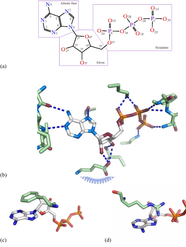
Figure 1a shows the molecular structure and chemical groups of an ATP. Besides the hydrogen bonding to the oxygen atoms of the phosphates and the ribose, the adenine base also has the capacity to form five hydrogen bonds, acting as a donor for two hydrogen bonds at the N6 position and hydrogen bond acceptors at the N1, N3, and N7 positions. (Figure 1b) This hydrogen bonding capacity of ATP is widely accepted as and important intermolecular interaction mode for DNA base-paring and protein-ligand interactions. There are two more equally important intermolecular interaction modes for adenine-protein interactions, i.e. π- π stacking interactions & cation-π interactions[12]. Just as in the case of DNA base-stacking, the conjugated π ring of the adenine base of ATP can interact with surrounding aromatic

residues (Phenylalanine, Tyrosine, and Tryptophan) via π-π stacking interactions. (Figure 1c) It can also interact with positively charged residues (Lysine, Arginine, and Histidine) through cation-π interactions. (Figure 1d) A wealth of information has been accumulated displaying the importance of π-π stacking interactions and cation-π interactions in the formation of bio-molecular systems. Typically, π-π stacking interactions and cation-π interactions are of similar or even greater magnitude than the hydrogen bonding energy[13-18].

1.4 3D-BLAST

3D-BLAST[19] has been created as a fast protein structure search tool and that can search >10,000 structures in 1.3 seconds using only an ordinary personal computer. This innovative program dispenses with the need to perform searches for Euclidean distances between corresponding residues; instead, the highly regarded local sequence alignment tool, BLAST, is used to discover homologous proteins and to evaluate the statistical significance of hits by providing E-values from structure databases. The core idea of 3D-BLAST is to design a structural alphabet—to be used to encode 3D protein structure databases into structural alphabet sequence databases (SADB)—and a structural alphabet substitution matrix (SASM). The method of 3D-BLAST encodes three-dimensional protein structures into structural alphabet sequences by mapping 5-mer structural segments into corresponding structural letters. These structural alphabet sequences and our new structural alphabet substitution matrix (SASM) enhance the ability of BLAST to search structural homology of a

query sequence to a known protein or family of proteins, often providing clues to the function of a query protein. We then enhanced the sequence alignment tool BLAST, which searches the SADB using the matrix SASM to rapidly determine protein structure homology or evolutionary classification.

3D-BLAST was designed to maintain the advantages of BLAST, including its robust statistical basis, effective and reliable database search capabilities, and established reputation in biology. However, the use of BLAST as a search tool also has several limitations, which are the maximum state (23 states) of the structural alphabet, the need for a new structural alphabet substitution matrix (SASM), and a new E-value threshold to indicate the statistical significance of an alignment. Furthermore, 3D-BLAST is slow if the structural alphabet is un-normalized, because the BLAST algorithm searches a statistically significant alignment by two main steps. It first scans the database for hit words that the scores exceed a threshold value if aligned with words in the query sequence. Then, it extends each hit word in both directions to check the alignment score. To reduce the negative effect of un-normalized structural alphabet, we set a maximum number, 16000(~7.0% of total structural segments in the pair database), of segments in a cluster in order to have similar compositions for the 23 structural letters and 20 amino acids.

3D-BLAST has the advantages of BLAST for fast structural database scanning and evolutionary classification. It searches for the longest common substructures, called

SAHSPs (Structural Alphabet High-scoring Segment Pairs), existing between the query structure and every structure in the structural database. The SAHSP is similar to the high-scoring segment pair (HSP) of BLAST, which is used to search amino acid sequences. 3D-BLAST ranks the search homology structures based on both SAHSP and E-values, which are calculated from the SASM. 3D-BLAST is much faster than related programs and it is available at http://3d-blast.life.nctu.edu.tw.

1.5 Thesis Overview

In this work, we adopted a structural-based binding pocket clustering scenario on ATP-binding protein chains. To more focus on the information in ATP-binding pockets, we took the binding pocket similarity into account during the clustering process. After clustering the binding pockets, we analyzed the non-bonded interactions between ATP and the binding protein chains systematically. We also calculated the interaction similarity and the interaction-conserved positions for each cluster.

In Chapter 2, we will introduce the materials and the methods, including the dataset preparation, the ATP-binding site extraction, the clustering scenario, and the analysis approaches on the non-bonded interactions. Chapter 3 shows the results and discussions. In that chapter, we will reveal the interaction distributions, the similarity of interactions in all clusters, and the interaction conservations within each cluster. After our clustering process, the ATP-binding pockets show relatively strong conservative properties within each cluster.

The results may contribute to the pattern generation and may help ones discover the structural motifs of the ATP-binding pockets. Therefore, we proposed some applications and the future works in Chapter 4 and drew a conclusion for this study.

Chapter 2

Material and Methods

In this chapter, we are going to introduce the materials used in this research, including the ATP-binding protein chains as the dataset and the ATP-binding SCOP[20] domains used in the verification. Also, we will illustrate the clustering scenario we adopted on those dataset in a step-by-step manner.

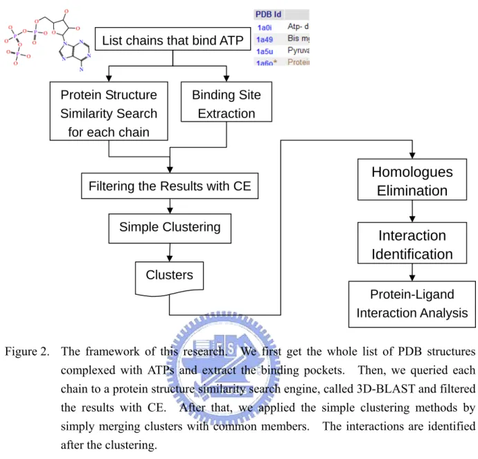
The overall framework is shown in Figure 2. In section 2.1, we first fetched the whole list of PDB structures complexed with ATPs and extracted the ATP-binding pockets (contact amino acid residues). Then, in section 2.2, we queried each chain to a protein structural similarity search engine, called 3D-BLAST[19], and the search results were further filtered by structural alignment with CE[21], focusing the structural similarity in the ATP-binding pockets. After that, we applied the simple clustering methods by simply merging clusters with common members.

The non-bonded interactions were identified after the clustering. We identified the non-bonded interactions by HBPLUS and an in-house software, PiFinder. The criteria used in these computer programs are shown in section 2.3. The equations used to calculate interaction similarity and interaction-conserved positions within each cluster are also introduced in the same section. After all, in section 2.4, we bring out the approach of

comparison between the SCOP classifications and our clustering results.

2.1 Preparation of Datasets

Preparation of ATP-binding Protein List

The list of ATP-binding proteins was obtained from the PDBsum[22] database (March 3rd, 2006). After all the obsolete or theoretical models were excluded, we had 246 PDB structures as the material for this research.

Extraction of ATP-binding Sites

After getting the ATP-binding protein list, we extracted the ATP-binding sites and the amino acid residues having contacts with ATPs. To do the job, we processed these PDB structures with an in-house program, which can identify any heterogen group in a PDB structure and every contact amino acid residues to the heterogen group. In our research, the defined contact range is 6 angstrom. If the distance between any atom of an amino acid residue and any atom on an ATP is within 6 angstrom, we considered the amino acid residue having contacts with the ATP and the amino acid residue is a `contact residue’ of ATP.

In the extracted ATP-binding sites, we found that there are some poorly bound ATP structures in PDB, ex. 1r8b, 1r9t and 1n5i. The ATPs in these structures bind abnormally due to the missing of some other compounds such as RNA strands[23], the mismatch binding ligand of the protein[24], or the affinity of ATP for this site could be promoted by the

protonation of some hydrophilic residues on the protein surface[25]. Besides, we also found some fragmentary ATP structures in the 246 structures. The ATP-binding sites in these abnormal ATP-binding structures usually are composed of no more than 13 amino acid residues. Therefore, we considered only ATP-binding sites composed of 14 or more amino acid residues as valid binding site structures.

After the extraction, we had 486 protein chains having contacts with ATP. A complete list of the ATP-binding protein chains used in this research comes in Appendix A.

Datasets for Verification

To verify the quality of our clustering results, we compared our results to the SCOP domains involving in ATP-binding sites. Every SCOP domain involving in the binding site was then filtered with the number of contact residues, which also belonging to the SCOP domain. A SCOP domain involving 6 or more amino acid residues were considered as a valid contact SCOP domain. Among the 486 protein chains, 341 of them have records in SCOP and at least one valid contact SCOP domain found.

2.2 The Clustering Scenario

Search for Structurally Similar ATP-binding Protein Chains

As we had the protein chains having contacts to ATPs, we wanted to know that among the 486 protein chains, which chains are structural neighbors to each other in both the whole

protein chain and the ATP-binding pocket view. To do so, we queried each contact protein chain to the 3D-BLAST server[19]. When using 3D-BLAST, we used the whole PDB as the searching database and set the cut-off e-value to 10-15. After querying 486 protein chains to the 3D-BLAST, we had 486 protein chain lists containing structurally similar ATP-binding protein chains (neighbors) to the query chains. However, since our research focused on ATP-binding sites, only PDB structures complexed with ATPs were analyzed in the later steps.

Structural Similarity Filtering

3D-BLAST is a fast structural similarity engine but not a structural alignment tool. It does not actually superpose protein structures. Further, proteins similar in the whole protein structures may not similar in the binding sites. Therefore, we used CE, a popular structural comparison tool of protein chains, to do the further filtering of the 3D-BLAST result lists.

For each 3D-BLAST result list, we did an all-against-query CE comparison. A subject chain in a list survives if the CE results between the query and the subject chains satisfy the following two rules.

One is the whole protein structural similarity. The query and the subject chains must have similar whole protein structures. The whole protein structure similarities were evaluated according to the following criterion.

5.0, 200 4.5, 100 200 4.0, Z if L Z if L Z otherwise ≥ ≥ ⎧ ⎪ ≥ ≤ < ⎨ ⎪ ≥ ⎩ (1),

where Z is the CE Z-score and L is the CE alignment length. A subject chain survives if the CE Z-score of the structural alignment to the query chain satisfies the criteria list in (1).

The other is the structural ATP-binding pocket similarity. The query and the subject chains must be similar in the ATP-binding sites after the CE structural alignment. To evaluate this criterion, we introduced the Binding Site Aligned Coverage as the following.

2 1,2 1 2 a n c n n = (2),

where n1 and n2 are the number of contact residues on the query and the subject chains,

respectively, and na is the number of amino acid residues that are aligned in the CE results and

the residues on both chains are contact residues to ATP. The c represents the structural _1,2

similarity of two binding sites on chain 1 and 2. The two binding site structures are similar if c_1,2 ≥0.4. Any subject chain on a 3D-BLAST resulting list having c_1,2 ≥0.4 to the

query chain would be filtered for the dissimilarity of the two binding sites, even if the two protein structures are similar.

Only subject chains satisfying both criteria were considered as structural neighbors to the query chain. We believed this structural similarity filtering process keeps protein chains with similar structures in both whole protein chain and the ATP-binding pocket together.

Merging the 3D-BLAST Result Lists

In this research, we adopt a very simple (or, naïve) clustering concept: if two clusters, A and B, have at least on member in common, A and B are then merged into one cluster. This clustering method may be simple, but somehow performed well.

After applying the structural similarity filtering on the 3D-BLAST result lists, we had 486 “clean” protein chain lists; each contains structurally similar protein chains to the query chain, in both the whole protein chain and the ATP-binding site aspects. We first took the “clean” protein chain lists as a cluster it self. Then, we merged these lists if any two of them have some surviving members in common. The simple clustering resulted in 70 clusters. Appendix A gives the whole list of clustering results and the protein chain information, including the number of contact residues to ATP, the contact SCOP domain family, the EC[6] number of the chain, and the protein name.

2.3 Non-bonded Interaction Analysis

Eliminating Homologues

discover novel ATP-binding motifs. However, the analysis may bias the dominant homologous chains, such as multi-chain PDB structures and highly homologous proteins among various species, presented in a cluster. Therefore, after the clustering, we used the sequence similarity to eliminate the homologues for each cluster. In this step, we adopt ed BLASTCLUST[26], a sequence clustering tool using BLAST[26], to do the job. BLASTCLUST is a DNA/protein sequence clustering tool by using the sequence identity as the clustering features. Chains with 90% or more sequence identity to any other chains in the same cluster were sub-clustered. When analyzing non-bonded interactions, we consider only the longest chain of each sub-cluster in a cluster.

Selecting the Representatives and Multiple Binding Site Alignments

After all the clustering and homologue eliminating steps, we chose a representative chain for each cluster. We selected a chain as the representative if the chain has the highest CE Z-scores to all the other chains in the same cluster.

As the representative chain being selected, we stacked the CE alignments of every chain to the representative (the star alignment). Figure 6b shows an example of structural binding pocket alignment of the cluster 58. The whole list of multiple structural alignments of binding pockets is shown in Appendix B.

Identification of Non-bonded Interactions in ATP-binding Pockets

Non-bonded intermolecular interactions between ATP and surrounding residues in the binding pockets are important to the recognition and binding of ATP. In this work, we focused on hydrogen bond, π-π stacking, and cation-π interactions between ATP and the residues on ATP-binding protein chains. The three types of non-bonded interactions in the 486 chains in PDB structures were identified by HBPLUS[27] and an in-house software, called PiFinder.

HBPLUS[27] identifies all hydrogen bonds in a PDB structure by calculating the distance and the angles between all hydrogen bond donors and acceptors. Then, it outputs the donor-acceptor pairs and their status of the found hydrogen bonds.

The π-π stacking and cation-π interactions between ATP and the residues on ATP-binding protein chains were identified by PiFinder, an in-house software written in C/C++. π-π stacking interactions are formed between the aromatic ring of an ATP and the aromatic rings of a Phenylalanine, Tyrosine, or Tryptophan. While cation-π interactions are formed between the adenine group of an ATP and the positively charged atoms of a Lysine or Arginine. PiFinder identifies a π-π stacking or cation-π interaction by checking the distance between the aromatic ring of an ATP and the aromatic ring or the cation on the amino acid residues. If the aromatic ring of Phe, Tyr, or Trp is in the 5.6 angstrom range of the aromatic ring of an ATP, PiFinder reports the ATP and the residue interact via the π-π stacking

interaction. If the cation of Lys or Arg is in the 5.6 angstrom range of the aromatic ring of an ATP, PiFinder will report the ATP and the residue interact via the cation-π interaction. The definitions of π-π stacking and cation-π interactions were referred to a previous study in [12].

In the figures showing non-boned interaction profiles for ATP-binding protein chains in this thesis (Figure 3,4,5,6,7), ‘|’ denotes the residues forming a hydrogen bonds to ATP, ‘=’ denotes the residues forming π-π stacking or cation-π interactions to the aromatic ring to ATP, and ‘+’ for combinations of these three types of non-bonded interactions on a residue.

Analysis of Protein-Ligand Interactions

For each cluster, we identified every hydrogen bond, π-π stacking or cation-π interactions to ATP by HBPLUS and PiFinder. Then we encoded the interaction profiles in the binding-pocket to binary strings. For each contact residue, residues that have at least one type of non-bonded interaction to the ATP are marked `1’, or `0’, otherwise.

After we transformed the hydrogen bond interactions for each chain in the cluster to binary strings, we used the Tanimoto Coefficient (or Jaccard Coefficient) (3) as an interaction similarity index. 1 2 1,2 1 2 s s tanimoto s s ∧ = ∨ (3),

the non-bonded interaction profiles of the two binding-pockets are.

Beside the interaction similarity, we also identified interaction-conserved positions in each clusters. For each position in a cluster, we calculate the percentage of forming interactions to ATP, intcon . (4) c i_,

, , c i c i c nInt intcon n = (4),

where n is the number of chains in the cluster c and c nInt is the number of chains c i, forming non-bonded interactions to ATP. A position in a cluster is interaction-conserved if

, 50%

c i

intcon ≥ .

2.4 Clustering Evaluation

To evaluate the performance of our clustering results, we compared our clustering results to the SCOP classifications. We first extracted the contact SCOP domain(s) for each ATP-binding pockets in the dataset. For each cluster, the most popular SCOP family in the cluster was assigned to the cluster, while the presenting of any other SCOP families was considered as incorrectly clustered. Then we calculated the rate of `correctly clustered’ (5) for each cluster and for the whole evaluated dataset.

#corrected clustered protein chains # protein chains with records in the SCOP

accuracy= (5)

To be noticed, one SCOP family may be assigned to two or more clusters, since proteins structurally similar may not function similarly. As our clustering method focused only on

protein structural properties, we consider protein chains under this circumstance as ‘correctly clustered’.

Chapter 3

Results and Discussions

Many works have been proposed to analyze on the ATP-binding proteins. Some of them used the multiple sequence alignment techniques to locate the conserved motifs or domains[21], such as the Walter A motif[10] and the Kinase-1 and the Kinase-2 motifs[11]. Some others adopted the structural alignment tools to find out the structural motifs for binding ATP [28], such as the ATP-grasp family[20]. Some other research groups systematically applied statistics on the distributions of different types of interactions between ATP and the binding proteins[12].

In this work, we adopted 3D-BLAST to search neighbors among ATP-binding protein chains, then used CE to structurally align ATP-binding proteins and used the results, especially the structural similarity in the binding pockets, to do the binding pocket clustering. Then we analyzed the non-bonded interactions, including hydrogen bonding, π-π stacking interactions, and cation-π interactions, between ATP and proteins for every cluster.

3.1 The Overall Results of the Clustering

The clustering resulted in 70 clusters from the 486 ATP-binding protein chains. Appendix A gives the whole clustering results of the 486 ATP-binding protein chains and the information of those protein chains. Among the 70 clusters, 20 of them are singletons and

16 clusters have only two chains. The rest of them, 34 clusters, have three members or more.

In each cluster, there exist many homologous chains, such as mutants or those from different species. The homologous chains may dominate over other chains while analyzing the sequence or the non-bonded interaction conservations in each cluster. Therefore, we applied the non-bonded interaction analyses on the homologue-eliminated clusters (Table 2) rather than the original ones. (Appendix A) The detailed steps for eliminating homologues are shown above in Chapter 2.

After eliminating homologues in each cluster, the number of singletons increased to 50, a relatively large number compared to the total 70 clusters. We compared the contact SCOP domains of those chains in singletons to the chains in the other clusters. We found that among those 50 singletons, except 15 of them with no domain documented in SCOP, the SCOP families of the contact SCOP domains of the 24 singletons are unique in the homologue-eliminated dataset. This somehow explains the large number of singletons that, protein structures in those singletons are structurally unique to the other ATP-binding proteins in the dataset. The rest 11 singletons belong to the same SCOP families as those of some other clusters.

3.2 The Comparison with the SCOP

There are 341 out of the 486 ATP-binding protein chains with domains documented in the SCOP classifications. Currently, they are classified into 50 different SCOP families. We calculated the rate of `correctly clustered‘(5) of those 341 protein chains as the accuracy of our clustering. Protein chains with no records in the SCOP classifications were omitted in the accuracy calculation.

With no surprise, the clustering results got a high correspondence with the SCOP classifications. Most binding pockets belonging with the same SCOP classification were clustered into the same group. The good correspondence was not surprising because we used the structural similarity as the clustering criteria whereas the SCOP classifies protein domains according to their structural components.

Overall, we got 95% accuracy on the original dataset, and 93% accuracy on the homologue-eliminated dataset. The accuracies of all 70 clusters are listed in Table 1.

3.3 The Sequence Identity

When two proteins have 30% or more sequence identity, one can infer that these two proteins have similar function with a high accuracy. To confirm that our clustering can cluster interaction-similar but non-homologous chains together, we checked the sequence identity distributions for all clusters. Table 4 and 5 show the distributions of intra-cluster

sequence identities of non-singleton clusters in the original and the homologue-eliminated datasets.

Before eliminating homologues, many clusters presented high sequence identity (Table 4). In Appendix A, we can see that a cluster with 100% sequence identities is usually made of a single multi-chain PDB structure. Theses clusters therefore would become singleton after the homologue filtering. This shows that, when searching in the 486 ATP-binding protein chains, there was no structurally similar protein chain in both whole protein and the ATP-binding pocket perspectives.

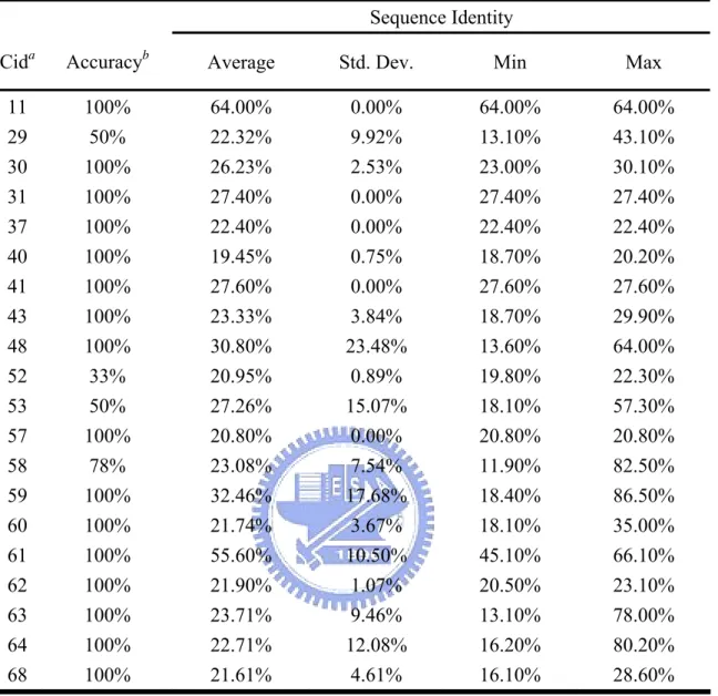
After filtering homologues, as Table 5 shows, only 2 clusters have protein chains with more than 30 percent sequence identity to all the other members, while other clusters present less homology. According to this non-homologous property, our analyses on ATP-binding mode and non-bonded interactions may not be biased by dominant homologous protein chains.

3.4 The Non-bonded Interaction Similarity

Non-bonded interactions play an important role in the ligand recognition of proteins. They also stabilize ligands in the binding pockets. There are three major types of non-bonded interaction between ligands and proteins. They are hydrogen bonding, π-π stacking, and cation-π interactions. There exist plenty of studies about hydrogen bond

interactions[29-32]. Though, there are some studies concerned about the contributions of π-π stacking interactions and cation-π interactions[15, 18, 33, 34]. They reported that π-π stacking interactions and cation-π interactions are of similar or even greater magnitude than the hydrogen bonding energy[13-18]. In this work, we analyzed the profiles of all these three types of non-bonded interactions and try to find out the difference of the interaction patterns between the clusters.

Interaction Similarity by the Tanimoto Coefficient

After the CE structural alignments and identifications of all the three types of non-bonded interactions, we tried to observe the non-bonded interaction profile similarity within each cluster. To achieve that, we adopted the Tanimoto Coefficient (or Jaccard Coefficient) (3) as an interaction similarity index. We encoded the interaction profiles in ATP-binding pockets as binary strings, where `1’ denotes the positions forming non-bonded interactions and `0’ represents for nothing. Then, we calculated the all-against-all Tanimoto Coefficients in a cluster and did the statistics on them. Table 3 shows the distributions of the interaction similarity of non-singleton clusters.

As the Table 3 shows, we found that many clusters present 25% or more interaction similarity. This shows that our clustering results do conserve on the interaction profile in most of the cases.

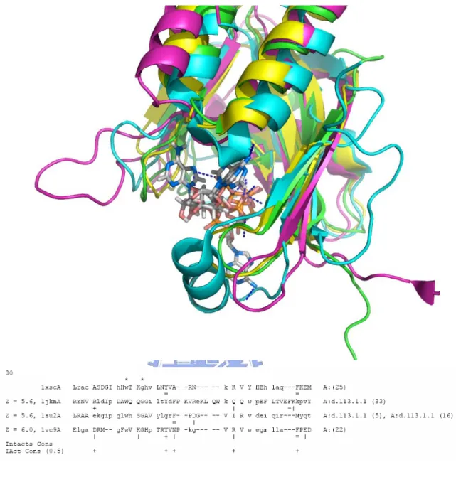
However, there are still clusters showing less similarity in their non-bonded interaction profiles, such as the cluster 30. Figure 5 shows the superposition, the CE structural alignments, and the interaction profile of the ATP-binding pockets of the cluster 30. The average interaction similarity of the cluster 30 is 10.5%, which is the lowest among all clusters. But, the 4 hydrolase protein chains are somehow well-aligned by CE. The reason why the interaction profiles are not so similar is the different ATP orientations in 1jknA and 1vc9A, while the proteins do present structural similarity.

3.5 The Interaction-Conserved Positions

For each position i a cluster, we calculate the percentage of forming interactions to ATP over a cluster c, intcon (4). In Table 3, we also give the counts of interaction-conserved _{c i,}

positions in each cluster. As our observation, those interaction-conserved positions are critical for ATP binding and they usually gather up in the regions, which may be potential motifs. We will discuss them in the next section.

3.6 The ATP-binding Motifs

Several well-known signature sequential motifs, such as the Walker A motif[10], Kinase-1, and Kinase-2 motifs[11] involve in binding of phosphate groups and their associated metal ions. In our clustering results, we can also see those well-known sequential motifs showing.

Known Patterns in the Clustering Results

The Walker A motif, G-X{4}-G-K-[TG]-X{6}-[IV], for adenylate kinase, α, β, and myosin. It interacts with the adenine base while an adenylate kinase catalyze an AMP with an ATP[10]. The Walker A motifs show up in the clusters 24, 29, 57, 62, and 64. (Appendix B) The Kinase-1 motif, [GASN]-X{4}-[GACS]-K-[GSTVAP]-[TSADGNM], functions in binding of phosphates of the ligand, which is ATP in our case[11]. It is much frequently found in the clustering results. It shows in the clusters 11, 16, 26, 27, 31, 38, 41, 46, 61, 63, 66, and 67. The Kinase-2 motif is relatively short and less seen in our clustering results. The motif is [VGILNTAYK]-[AFLIGDETCKP]-[ALIGVSPEFHT]-[LGVITDFQMYK]-D. It contains the conserved aspartate that coordinates with the Mg-ATP in the ATP-binding site[11]. In our clustering results, it presents in the cluster 59 only.

Besides those well-known sequence motifs, we found some novel motifs that form hydrogen bonds to ATP.

Potential Patterns in the cluster 29

In the cluster 29, there is a highly conserved region, named C29_PAT in the beginning part of the binding site alignment. (Figure 3) The 4 members are ATP-binding sites from ubiquitin-activating related and adenylyltransferase thiF proteins. Among the 4 chains in the cluster 29, there are several identical positions in both structural and interaction views. As

we query C29_PAT to the PROSITE database by encoding C29_PAT as [IV]G[AL]GG[IL]G-X(17)-[28]-D-[MFLD]-D-[TD]-[IV]-[SDH]-[LV]-SNL-[NQ]RQ-X(11)-K, which is the pattern syntax used in PROSITE, the returned sequences are all related to the for chains in the cluster 29. Besides, the PROSITE reported `no hits’ for any documented patterns in the database, while we query the 4 chains to the ScanProsite server[28]. We believed that was the evidence for C29_PAT being a potential novel pattern for ubiquitin-activating related and adenylyltransferase thiF proteins. However, it needs further validation by stronger supports.

Potential Patterns in the cluster 59

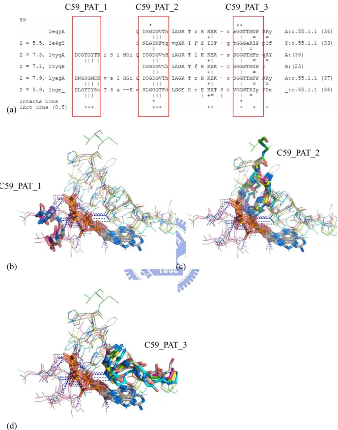
The cluster 59 is one of the clusters with most interaction-conserved positions shown. From the multiple structure alignment of the cluster 59 (Figure 4), we identified three potential motifs for interacting to ATP. They are D-[CNL]-G-[ST]-[35]-[MY]-[CST]-[KC],

[DS]-[LS]-G-[GDY]-[28]-[FTV]-[TF]-[HGD], and [STV]-G-G-[GST]-[AT]-[KMR]-[IFY]-[PR], ordered by their occurrences in the alignment.

We named them as C59_PAT_1, C59_PAT_2, and C59_PAT_3, respectively. The C59_PAT_3 forms non-bonded interaction to the adenine base of ATP while C59_PAT_1 and C59_PAT_2 form hydrogen bonds to the phosphate groups.

The cluster 59 contains chains of α-actin, Arp 2/3, defensin HBD-2, and Hsc70 proteins. Except Arp2 and Arp3, which have no record in the SCOP, they have c.55.1.1 family domains

as the ATP contact SCOP domain. Not only does the SCOP classify these contact domains into a same family, there are literatures support the structural similarity and the genetic relationship among them[36]. As we query the three motifs found in this cluster to PROSITE[28], there is no previous defined pattern matching them. Furthermore, when we queried the whole sequences of each chain to PROSITE to search for known patterns, PROSITE returned `no hit’ on the sequences. This tells us that we may have found some novel patterns for Actin/Hsc70 protein families.

There are still other potential motifs interacting with ATP, though, they need to be further validated. They are shown in Appendix B, where we give the overall view of structural alignments and interaction profiles for each cluster.

Chapter 4

Conclusions and Future Works

4.1 Conclusions

The rapid increase of three-dimensional protein-ligand complex structures has made the analysis on protein-ligand binding research. However, the slowly updated classification databases, like SCOP and CATH, make it hard to classify newly solved protein structure immediately.

In this work, we adopted a fast protein structural similarity search tool, called 3D-BLAST, to do protein-ligand complexes analysis and used ATP-binding proteins as a study case. We clustered protein-ATP complexes based on the whole protein chain structures, the binding-site structural similarity, and non-bonded interaction profiles. With the clustering, we are able to analyze the protein-ligand interactions and identify functional important residues and potential ATP-binding motifs.

First of all, we used 3D-BLAST to perform protein-ligand complexes homologous search in whole protein database. Secondly, CE was used as a detailed structure alignment tool to identify structural similarity of ligand-binding site. Accordingly, we can obtain a preliminary classification for protein complexes.

software, PiFinder, to identify the non-bonded interactions including hydrogen bond, π- π stacking, and cation- π interactions. According to structural similarity and functional protein-ligand interaction patterns, a simple cluster method was applied to group protein-ATP complexes.

Overall, we got a 95% accuracy of the clustering results compared to the SCOP classifications. We systematically analyzed the non-bonded interactions, between ATP and the binding protein chains. We found that the three types of non-bonded interactions show relatively strong conservation within clusters. Not only had the ATP-binding motif discovered in the previous works, some novel potential ATP-binding motifs were also identified in some clusters.

4.2 Applications and Future Works

Since the discovered novel motifs are more important to the ATP-binding, the novel motifs can then be used to predict the ATP-binding property of proteins not complexed with ATPs or even protein sequences that the structures are not solved yet.

With the fast protein-ATP complex clustering method and the protein-ligand interaction analyses proposed in this work, we can also apply the same process to protein-ligand complexes of any other ligand. Therefore, we can discover more potential novel ligand-binding motifs that essential for the ligand-binding. Moreover, we can construct a

ligand-binding motif database and provide some services for searching proteins that could be bound by a given ligand or ligands that probably bind to a given protein. However, since the lack of evidence of the novel ligand-binding motifs currently, the newly discovered motifs should be carefully validated in the future days.

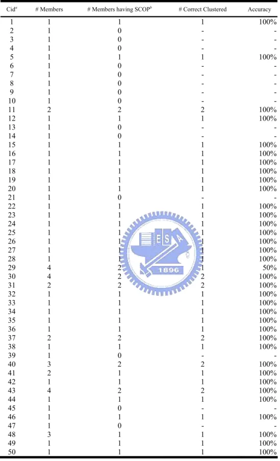
Table 1. The accuracy for each cluster

Cida _{# Members # Members having SCOP}b _{# Correct Clustered Accuracy}

1 1 1 1 100% 2 1 0 - - 3 1 0 - - 4 1 0 - - 5 1 1 1 100% 6 1 0 - - 7 1 0 - - 8 1 0 - - 9 1 0 - - 10 1 0 - - 11 2 2 2 100% 12 1 1 1 100% 13 1 0 - - 14 1 0 - - 15 1 1 1 100% 16 1 1 1 100% 17 1 1 1 100% 18 1 1 1 100% 19 1 1 1 100% 20 1 1 1 100% 21 1 0 - - 22 1 1 1 100% 23 1 1 1 100% 24 1 1 1 100% 25 1 1 1 100% 26 1 1 1 100% 27 1 1 1 100% 28 1 1 1 100% 29 4 2 1 50% 30 4 2 2 100% 31 2 2 2 100% 32 1 1 1 100% 33 1 1 1 100% 34 1 1 1 100% 35 1 1 1 100% 36 1 1 1 100% 37 2 2 2 100% 38 1 1 1 100% 39 1 0 - - 40 3 2 2 100% 41 2 1 1 100% 42 1 1 1 100% 43 4 2 2 100% 44 1 1 1 100% 45 1 0 - - 46 1 1 1 100% 47 1 0 - - 48 3 1 1 100% 49 1 1 1 100% 50 1 1 1 100%

Cida _{# Members # Members having SCOP}b _{# Correct Clustered Accuracy}

51 1 1 1 100% 52 4 3 1 33% 53 4 4 2 50% 54 1 1 1 100% 55 1 1 1 100% 56 1 1 1 100% 57 3 3 3 100% 58 16 9 7 78% 59 6 4 4 100% 60 7 7 7 100% 61 3 1 1 100% 62 3 2 2 100% 63 11 7 7 100% 64 8 4 4 100% 65 1 0 - - 66 1 1 1 100% 67 1 1 1 100% 68 5 4 4 100% 69 1 1 1 100% 70 1 1 1 100%

a _{The serial identification of clusters.}

Table 2. The cluster results after eliminating homologues Cida _Repb _Chain SCOP Families of

Contact Domains c EC Protein Name

1 4at1B 4at1B d.58.2.1 (21) 2.1.3.2 Aspartate Carbamoyltransferase 2 2c01X 2c01X 3.1.27.5 Nonsecretory Ribonuclease 3 2aruA 2aruA 6.3.2.- Lipoate-Protein Ligase A 4 2aqxA 2aqxA 2.7.1.127 Inositol 1,4,5-Trisphosphate 3-Kinase B 5 8icnA 8icnA d.218.1.2 (15) 2.7.7.7 DNA Polymerase Beta

6 1z0sA 1z0sA 2.7.1.23 Polyphosphate/ATP-NAD Kinase

7 1yp3A 1yp3A 2.7.7.27 Glucose-1-Phosphate Adenylyltransferase Small Subunit (ADP-Glucose Synthase)

8 1y56A 1y56A 1.5.99.8 L-Proline Dehydrogenase 9 1xdnA 1xdnA RNA Editing Ligase Mp52 10 1wklB 1wklB 2.7.4.6 Nucleotide Diphosphate Kinase 11 1vjcA 1vjcA c.86.1.1 (26) 2.7.2.3 Phosphoglycerate Kinase

3pgk_ c.86.1.1 (28) 2.7.2.3 Phosphoglycerate Kinase

12 2gnkA 2gnkA d.58.5.1 (17) Nitrogen Regulatory Protein 13 1v3sA 1v3sA Nitrogen Regulatory Protein Pii

14 1twaA 1twaA 2.7.7.6 DNA-Directed RNA Polymerase II Largest Subunit 15 1tc0A 1tc0A d.122.1.1 (25) Endoplasmin

16 1qhxA 1qhxA c.37.1.3 (28) 2.7.1.- Chloramphenicol Phosphotransferase

17 1obgA 1obgA d.143.1.1 (13) 6.3.2.6 Phosphoribosylamidoimidazole-Succinocarboxamide Synthase 18 1obdA 1obdA d.143.1.1 (23) 6.3.2.6 Phosphoribosylamidoimidazole-Succinocarboxamide Synthase 19 1o93B 1o93B d.130.1.1 (14) 2.5.1.6 S-Adenosylmethionine Synthetase

20 1o93A 1o93A d.130.1.1 (16) 2.5.1.6 S-Adenosylmethionine Synthetase 21 1yfrA 1yfrA 6.1.1.7 Alanyl-tRNA Synthetase 22 1n48A 1n48A e.8.1.7 (22) DNA Polymerase IV

23 1mo8A 1mo8A d.220.1.1 (24) Sodium/Potassium-Transporting Atpase Alpha-1 24 1mjhA 1mjhA c.26.2.4 (32) (unknown)

25 1miwA 1miwA d.218.1.4 (17), a.173.1.1 (11) tRNA Cca-Adding Enzyme 26 1w7aB 1w7aB c.37.1.12 (28) DNA Mismatch Repair Protein Muts 27 1ko5A 1ko5A c.37.1.17 (23) 2.7.1.12 Gluconate Kinase

28 1r8bA 1r8bA d.218.1.7 (23), a.160.1.3 (6), d.58.16.2 (10)

tRNA Nucleotidyltransferase 29 1jwaB 1jwaB c.111.1.1 (29) Molybdopterin Biosynthesis MoeB Protein

1r4nB c.111.1.2 (30) Ubiquitin-Activating Enzyme E1C 1y8qB Ubiquitin-Like 2 Activating Enzyme E1B 1zfnA 2.7.7.- Adenylyltransferase THIF

30 1xscA 1jknA d.113.1.1 (33) 3.6.1.17 Diadenosine 5',5'''-P1,P4-Tetraphosphate Hydrolase 1su2A d.113.1.1 (21) Mutt/Nudix Family Protein 1vc9A HB8 Ap6A Hydrolase

1xscA 3.6.1.17 Bis(5'-Nucleosyl)-Tetraphosphatase 31 1jjvA 1jjvA c.37.1.1 (20) 2.7.1.24 Dephospho-CoA Kinase

1uf9C c.37.1.1 (24) (unknown) 32 1jagA 1jagA c.37.1.1 (33) 2.7.1.113 Deoxyguanosine Kinase

33 3r1rA 3r1rA a.98.1.1 (19) 1.17.4.1 Ribonucleotide Reductase R1 Protein 34 1hp1A 1hp1A d.114.1.1 (14) 3.1.3.5, 3.6.1.45 5'-Nucleotidase

35 1hi1A 1hi1A e.8.1.6 (16) RNA Polymerase

36 1pj4A 1pj4A c.2.1.7 (22), c.58.1.3 (7) 1.1.1.39 NAD-Dependent Malic Enzyme, Mitochondrial 37 1n77A 1gtrA c.26.1.1 (29) 6.1.1.18 Glutaminyl-tRNA Synthetase

Cida _Repb _Chain SCOP Families of

Contact Domains c EC Protein Name

38 1g5tA 1g5tA c.37.1.11 (18) 2.5.1.17 COB(I)Alamin Adenosyltransferase 39 1xdpA 1xdpA 2.7.4.1 Polyphosphate Kinase

40 1gn8A 1f9aA c.26.1.3 (28) NMN Adenylyltransferase 1gn8A c.26.1.3 (33) 2.7.7.3 Phosphopantetheine Adenylyltransferase 1yunA 2.7.7.18 Nicotinate-Nucleotide Adenylyltransferase 41 1xexA 1f2uA c.37.1.12 (21) RAD50 ABC-Atpase

1xexA SMC Protein 42 1kvkA 1kvkA d.14.1.5 (29) Mevalonate Kinase 43 1yidB 1h3eA c.26.1.1 (32) 6.1.1.1 Tyrosyl-tRNA Synthetase

1m83A c.26.1.1 (36) 6.1.1.2 Tryptophanyl-tRNA Synthetase 1yidB 6.1.1.2 Tryptophanyl-tRNA Synthetase 2a84A 6.3.2.1 Pantoate--Beta-Alanine Synthetase 44 1nsyA 1nsyA c.26.2.1 (27) 6.3.5.1 NAD Synthetase

45 1r9tB 1r9tB 2.7.7.6 DNA-Directed RNA Polymerase II 46 1fmwA 1fmwA c.37.1.9 (32) Myosin II Heavy Chain 47 1sx3A 1sx3A Groel Protein 48 2bu2A 1tilA d.122.1.3 (35) 2.7.1.37 Anti-Sigma Factor Spoiiab

1y8pA 2.7.1.99 [Pyruvate Dehydrogenase [Lipoamide]] Kinase Isozyme 3 2bu2A 2.7.1.99 Pyruvate Dehydrogensae Kinase Isoenzyme 2 49 1n5iA 1n5iA c.37.1.1 (10) Thymidylate Kinase 50 1e2qA 1e2qA c.37.1.1 (21) 2.7.4.9 Thymidylate Kinase

51 1dy3A 1dy3A d.58.30.1 (27) 2.7.6.3 7,8-Dihydro-6-Hydroxymethylpterinpyrophosphokinase (Pyrophosphorylase, Pppk)

52 2f02A 1esqA c.72.1.2 (27) 2.7.1.50 Hydroxyethylthiazole Kinase 1lhrA c.72.1.5 (29) 2.7.1.35 Pyridoxal Kinase

1v1bA c.72.1.1 (34) 2-Keto-3-Deoxygluconate Kinase 2f02A 2.7.1.144 Tagatose-6-Phosphate Kinase

53 1dv2A 1dv2A d.142.1.2 (28) 6.3.4.14 Biotin Carboxylase

1kj8A d.142.1.2 (30) 2.1.2.- Phosphoribosylglycinamide Formyltransferase 2 1i7lA d.142.1.3 (32) Synapsin II

1pk8A d.142.1.3 (29) Synapsin I 54 1d9zA 1d9zA c.37.1.19 (23) DNA Repair Protein UVRB 55 1bcpF 1bcpF b.40.2.1 (9) 2.4.2.- Pertussis Toxin 56 1bcpE 1bcpE b.40.2.1 (13) 2.4.2.- Pertussis Toxin

57 1h8hA 1e79A c.37.1.11 (17) 3.6.1.34 ATP Synthase Alpha Chain Heart Isoform (Bovine Mitochondrial F1-Atpase)

1h8hA c.37.1.11 (19) 3.6.1.34 ATP Synthase Alpha Chain Heart Isoform 1tf7A c.37.1.11 (23) Circadian Clock Protein KAIC 58 1gol_ 1atpE d.144.1.7 (33) 2.7.1.37 cAMP-Depedent Protein Kinase (CAPK)

1b38A d.144.1.7 (30) 2.7.1.37 Cell Division Protein Kinase 2 1ol6A d.144.1.7 (26) 2.7.1.37 Serine/Threonine Kinase 6 1csn_ d.144.1.7 (29) 2.7.1.- Casein Kinase-1 1phk_ d.144.1.7 (31) 2.7.1.38 Phosphorylase Kinase 1gol_ d.144.1.7 (22) 2.7.1.- Extracellular Regulated Kinase 2 1q97A d.144.1.7 (29) 2.7.1.- Sr Protein Kinase

1e8xA d.144.1.4 (26) 2.7.1.137 Phosphatidylinositol 3-Kinase Catalytic Subunit 1tqpA d.144.1.9 (28) RIO2 Serine Protein Kinase

1zp9A RIO1 Kinase

1s9iA Dual Specificity Mitogen-Activated Protein Kinase Kinase 2 1s9jA Dual Specificity Mitogen-Activated Protein Kinase Kinase 1 1u5rA Serine/Threonine Protein Kinase Tao2

1ua2A 2.7.1.37 Cell Division Protein Kinase 7 1zydA 2.7.1.37 Serine/Threonine-Protein Kinase GCN2 2biyA 2.7.1.37 3-Phosphoinositide Dependent Protein Kinase-1 59 1eqyA 1e4gT c.55.1.1 (33) Cell Division Protein FTSA

1eqyA c.55.1.1 (36) Alpha-Actin 1nge_ c.55.1.1 (36) 3.6.1.3 Heat-Shock Cognate 70Kd Protein 1yagA c.55.1.1 (37) Actin

1tyqA Actin-Related Protein 3 1tyqB Actin-Related Protein 2

Cida _Repb _Chain SCOP Families of

Contact Domains c EC Protein Name

60 1b76A 1aszA d.104.1.1 (22) 6.1.1.12 Aspartyl tRNA Synthetase 1b76A d.104.1.1 (29) 6.1.1.14 Glycyl-tRNA Synthetase 1b8aA d.104.1.1 (26) 6.1.1.12 Aspartyl-tRNA Synthetase 1e24A d.104.1.1 (29) 6.1.1.6 Lysyl-tRNA Synthetase 1h4qA d.104.1.1 (27) 6.1.1.15 Prolyl-tRNA Synthetase 1kmnA d.104.1.1 (30) 6.1.1.21 Histidyl-tRNA Synthetase 1nyrA d.104.1.1 (28) 6.1.1.3 Threonyl-tRNA Synthetase 1 61 1ayl_ 1ayl_ c.91.1.1 (37) 4.1.1.49 Phosphoenolpyruvate Carboxykinase

1xkvA 4.1.1.49 Phosphoenolpyruvate Carboxykinase 1ytmA 4.1.1.49 Phosphoenolpyruvate Carboxykinase 62 2bekA 1a82_ c.37.1.10 (29) 6.3.3.3 Dethiobiotin Synthetase

1g21E c.37.1.10 (31) 1.18.6.1 Nitrogenase Iron Protein 2bekA Segregation Protein SOJ

63 1b0uA 1b0uA c.37.1.12 (19) ABC Transporter (Histidine Permease) 1f2uB c.37.1.12 (19) RAD50 ABC-Atpase 1ji0A c.37.1.12 (21) ABC Transporter 1l2tA c.37.1.12 (22) ABC Transporter

1mv5A c.37.1.12 (17) Multidrug Resistance ABC Transporter ATP-Binding And Permease Protein

1q12A c.37.1.12 (31) Maltose/Maltodextrin Transport ATP-Binding Protein Malk 1r0xA c.37.1.12 (21) Cystic Fibrosis Transmembrane Conductance Regulator (CFTR) 1vciA Sugar-Binding Transport ATP-Binding Protein

1xefA Alpha-Hemolysin Translocation ATP-Binding Protein HLYB 1xexB SMC Protein

1xmiA 3.6.3.49 Cystic Fibrosis Transmembrane Conductance Regulator 64 1nsf_ 1do0A c.37.1.20 (29) Chaperone (Heat Shock Locus U)

1g3iA c.37.1.20 (29) ATP-Dependent HSLU Protease 1j7kA c.37.1.20 (31) Holliday Junction DNA Helicase Ruvb 1nsf_ c.37.1.20 (26) N-Ethylmaleimide Sensitive Factor 1ojlE Transcriptional Regulatory Protein Zrar 1svmA Large T Antigen

2a5yB CED-4

2c96A PSP Operon Transcriptional Activator 65 1z7eA 1z7eA Protein ArnA 66 1qhgA 1qhgA c.37.1.19 (25) ATP-Dependent Helicase Pcra 67 1ii0A 1ii0A c.37.1.10 (29) 3.6.3.16 Arsenical Pump-Driving Atpase 68 1xngA 1ee1A c.26.2.1 (33) 6.3.5.1 NH3-Dependent NAD+ Synthetase

1j1zA c.26.2.1 (24) 6.3.4.5 Argininosuccinate Synthetase 1kp2A c.26.2.1 (28) 6.3.4.5 Argininosuccinate Synthetase 1mb9A c.26.2.1 (33) Beta-Lactam Synthetase

1xngA 6.3.1.5 NH(3)-Dependent NAD(+) Synthetase 69 1a49A 1a49A c.1.12.1 (24), b.58.1.1 (11) 2.7.1.40 Pyruvate Kinase

70 1a0i_ 1a0i_ d.142.2.1 (22) 6.5.1.1 DNA Ligase

a _{The serial identification of clusters.}

b _{The representative protein chain of the `Cid’-th cluster.}

c _{The SCOP families of the contact domains. The numbers in the parentheses are the}

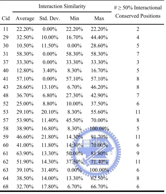
Table 3. Statistics on interaction similarity of non-singleton clusters

Interaction Similarity

Cid Average Std. Dev. Min Max

# ≥ 50% Interactional Conserved Positions 11 22.20% 0.00% 22.20% 22.20% 2 29 32.50% 10.00% 16.70% 44.40% 4 30 10.50% 11.50% 0.00% 28.60% 5 31 58.30% 0.00% 58.30% 58.30% 7 37 33.30% 0.00% 33.30% 33.30% 3 40 12.80% 3.40% 8.30% 16.70% 5 41 57.10% 0.00% 57.10% 57.10% 8 43 28.60% 13.10% 6.70% 46.20% 8 48 36.70% 6.80% 27.30% 42.90% 7 52 25.00% 8.80% 10.00% 37.50% 6 53 29.10% 20.10% 8.30% 55.60% 11 57 53.90% 11.40% 45.50% 70.00% 8 58 38.90% 16.80% 8.30% 100.00% 5 59 46.60% 21.80% 14.30% 91.70% 11 60 41.00% 11.80% 14.30% 70.00% 6 61 63.90% 13.30% 50.00% 81.80% 9 62 51.90% 14.30% 37.50% 71.40% 11 63 39.10% 31.40% 0.00% 100.00% 6 64 38.50% 14.00% 13.30% 62.50% 8 68 32.70% 17.80% 6.70% 66.70% 6

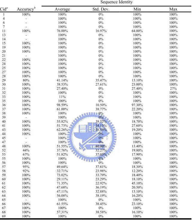
Table 4. Statistics on sequence identity of non-singleton clusters before eliminating homologues

Sequence Identity

Cida _Accuracyb _{Average Std. Dev. Min Max}

1 100% 100% 0% 100% 100% 4 - 100% 0% 100% 100% 6 - 100% 0% 100% 100% 7 - 100% 0% 100% 100% 11 100% 76.00% 16.97% 64.00% 100% 13 - 100% 0% 100% 100% 14 - 100% 0% 100% 100% 15 100% 100% 0% 100% 100% 19 100% 100% 0% 100% 100% 20 100% 100% 0% 100% 100% 21 - 100% 0% 100% 100% 22 100% 100% 0% 100% 100% 24 100% 100% 0% 100% 100% 25 100% 100% 0% 100% 100% 27 100% 100% 0% 100% 100% 28 100% 100% 0% 100% 100% 29 80% 41.14% 35.47% 13.10% 100% 30 100% 38.53% 27.61% 23.00% 100% 31 100% 27.40% 0% 27.40% 27% 32 100% 100% 0% 100% 100% 33 100% 11% 0% 100% 100% 35 100% 100% 0% 100% 100% 36 100% 98.59% 10.50% 97.30% 100% 37 100% 61.00% 38.77% 22.20% 100% 38 100% 100% 0% 100% 100% 39 - 100% 0% 100% 100% 40 100% 55.82% 39.52% 18.70% 100% 41 100% 51.73% 34.13% 27.60% 100% 43 100% 62.26% 38.58% 19.20% 100% 44 100% 100% 0% 100% 100% 45 - 100% 0% 100% 100% 47 - 100% 0% 100% 100% 48 100% 51.55% 40.00% 13.40% 100% 52 44% 37.76% 32.27% 19.80% 100% 53 67% 51.82% 37.03% 17.90% 100% 55 100% 100% 0% 100% 100% 56 100% 100% 0% 100% 100% 57 95% 49.64% 37.61% 18.30% 100% 58 92% 32.71% 23.98% 12.20% 100% 59 100% 73.02% 33.79% 18.40% 100% 60 100% 29.11% 23.29% 18.10% 100% 61 100% 71.35% 22.92% 45.10% 100% 62 100% 47.68% 36.19% 20.50% 100% 63 100% 47.11% 32.88% 13.10% 100% 64 100% 56.08% 38.19% 16.20% 100% 65 - 100% 0% 100% 100% 66 100% 61.55% 38.45% 23.10% 100% 67 100% 100% 0% 100% 100% 68 100% 57.31% 38.58% 16.10% 100% 69 100% 100% 0% 100% 100%

a _{The serial identification of clusters.}

b _{The accuracy compared to SCOP. Clusters with no contact SCOP domain found are}

Table 5. Statistics on sequence identity of non-singleton clusters after eliminating homologues

Sequence Identity

Cida _Accuracyb _{Average Std. Dev. Min Max}

11 100% 64.00% 0.00% 64.00% 64.00% 29 50% 22.32% 9.92% 13.10% 43.10% 30 100% 26.23% 2.53% 23.00% 30.10% 31 100% 27.40% 0.00% 27.40% 27.40% 37 100% 22.40% 0.00% 22.40% 22.40% 40 100% 19.45% 0.75% 18.70% 20.20% 41 100% 27.60% 0.00% 27.60% 27.60% 43 100% 23.33% 3.84% 18.70% 29.90% 48 100% 30.80% 23.48% 13.60% 64.00% 52 33% 20.95% 0.89% 19.80% 22.30% 53 50% 27.26% 15.07% 18.10% 57.30% 57 100% 20.80% 0.00% 20.80% 20.80% 58 78% 23.08% 7.54% 11.90% 82.50% 59 100% 32.46% 17.68% 18.40% 86.50% 60 100% 21.74% 3.67% 18.10% 35.00% 61 100% 55.60% 10.50% 45.10% 66.10% 62 100% 21.90% 1.07% 20.50% 23.10% 63 100% 23.71% 9.46% 13.10% 78.00% 64 100% 22.71% 12.08% 16.20% 80.20% 68 100% 21.61% 4.61% 16.10% 28.60%

a _{The serial identification of clusters.}

(a)

(b)

(c) (d)

Figure 1. Properties of ATP. (a) Molecular structure and chemical groups of ATP. The atoms are labeled according to the IUPAC_IUB JCBN naming system. (b) The ATP structure and the hydrogen bonds to the surrounding residues in 1atp. ATP acts as a hydrogen bond donor (N6) and a hydrogen bond acceptor (N1, N3, N7, O3*, O4*, O2*, and oxygen atoms on phosphates). (c) The π-π stacking between the π rings of ATP and aromatic amino acids, Phe, Tyr, and Trp. (d) The cation-π interaction between the π ring of ATP and positively charged amino acids, Arg and Lys.

Figure 2. The framework of this research. We first get the whole list of PDB structures complexed with ATPs and extract the binding pockets. Then, we queried each chain to a protein structure similarity search engine, called 3D-BLAST and filtered the results with CE. After that, we applied the simple clustering methods by simply merging clusters with common members. The interactions are identified after the clustering.

Protein Structure Similarity Search for each chain

Filtering the Results with CE Binding Site

Extraction List chains that bind ATP

Protein-Ligand Interaction Analysis

Interaction

Identification

Simple Clustering Clusters

Homologues

Elimination

(a)

(b)

Figure 3. The multiple structure alignment of ATP binding-pockets in the cluster 29. (a) The close view of ATP-binding pockets in the cluster 29. (b) The multiple structure alignment and interaction profile of the cluster 29. The contact residues are shown in uppercases while the others in lowercases. The hydrogen bonds (represented by bars, `|’) to the phosphate groups are highly conserved within the cluster. Moreover, we also identified a potential novel motif, [IV]-G-[AL]-G-G-[IL]-G-X(17)-[28]-D-[MFLD]-D-[TD]-[IV]-[SDH]-[LV]-S-N-L-[NQ]-R-Q-X(11)-K (the red box), called C29_PAT, in that area. We believe that C29_PAT can be a signature for ubiquitin-activating related proteins and adenylyltransferases, which are the members of cluster 29.

(a)

(b) (c)

(d)

Figure 4. The potential motifs in the cluster 59. (a) The multiple structure alignment of the cluster 59 with showing the potential motifs, C59_PAT_1, C59_PAT_2, and C59_PAT_3. (b) (c) (d) The superposition of the ATP-binding pockets with showing the C59_PAT_1, C59_PAT_2, and C59_PAT_3 as sticks, respectively.

C59_PAT_1 C59_PAT_2 C59_PAT_3

C59_PAT_1

C59_PAT_2

(a)

(b)

Figure 5. The CE structural alignments and the interaction profile of the ATP-binding pockets of the cluster 30. (a) The superposition of ATP-binding protein chains in the cluster 30. (b) The multiple structure alignment and interaction profile in ATP-binding pockets of the cluster 30. From the figures

(a)

(b)

Figure 6. An example of structural binding pocket alignment of the cluster 58. (a) The superposition of ATP-binding protein chains in the cluster 58. (b) The multiple structure alignment and interaction profile in ATP-binding pockets of the cluster 58. The superposition of the ATP-binding pocket structures in 9 protein chains, which have records in the SCOP, of the cluster 58. We can see that the hydrogen bond pattern around the adenine groups is strongly conserved among the cluster.

(a) (b)

(c)

(d)

Figure 7. An example of structural binding pocket alignment of the cluster 53. (a) The ATP-binding pockets and the hydrogen bonds in protein chains of the cluster 53. (b) The superposition of the protein chains in the cluster 53. The protein chains colored in cyan, magenta, yellow, and salmon red are 1dv2A, 1pk8A, 1j7lA, and 1kj8A, respectively. (c) The multiple structure alignment and the interaction profile of the cluster 53, with showing the `shifting’ region. (d) the superposition of ATP and the residues interacting with ATP in 1dv2A and 1kj8A from two different angles. We can see that the ATP structure is not well superposed to the others but the hydrogen bonds are somehow conserved. The error of superposing 1kj8A causes the shift of the non-bonded interaction pattern in the multiple structure alignment of the cluster.