國 立 交 通 大 學
高階主管管理學程碩士班
碩
士
論
文
經由格網計算推動金融服務競爭力
Financial Services Competitiveness through Grid Computing
研 究 生:林芳邦
指導教授:李正福
鍾惠民
經由格網計算推動金融服務競爭力
Financial Services Competitiveness through Grid Computing
研 究 生:林芳邦 Student:Fang-Pang Lin
指導教授:李正福 Advisor:Cheng-Few Lee
鍾惠民 Huimin Chung
國 立 交 通 大 學
高階主管管理學程碩士班
碩 士 論 文
A ThesisSubmitted to Master Program of Management for Executives College of Management
National Chiao Tung University in partial Fulfillment of the Requirements
for the Degree of Executive Master
of
Business Administration
June 2008
Hsinchu, Taiwan, Republic of China
i
學生:林芳邦
指導教授
:李正福
鍾惠民
國立交通大學高階主管管理學程碩士班
摘
要
金融服務近幾年來面臨快速的資訊科技發展所帶來的的挑戰,在金融服務業務上,如交易、 避險與風險管理等等,經常需要同時兼顧快速反應與大量費時的計算模擬,其競爭力的關鍵經 常僅在於有效資訊提供與市場交易的秒差優勢。要達成如此的競爭優勢,需要的不僅是購買高 效能的計算與儲存設施,還需要包括客製化的商業邏輯與重要(Mission Critical)分析功能, 甚至需要將分析的演算法調整到效能能達到毫秒之等級。在客製化的商業邏輯部分目前流行的 架構以網頁服務(Web service)與服務導向架構(Service Oriented Architecture, SOA)為主, XML 為基本資料交換架構,始能極易與不同應用資訊平台間進行資訊整合、融合與視覺化。在 重要分析功能方面,形成一個競爭瓶頸,可以高效能計算解決,但高速計算資源極為昂貴且其 計算循環(Compute Cycle)有限。隨著高速光纖的興起與普及,使利用分散式的大型計算資源 串連來擴充計算的循環變成更為有效,格網計算(Grid Computing)是近年來最重要的工具。本 研究即以格網計算來加速與擴充計算循環,其中探討現有較常用且需要大型計算資源的演算法 其在格網計算上的加速方法與效益;並且以蒙地卡羅模擬法(Monte Carlo Simulation)之選擇 權評價與風險管理值為範例,分別以大型叢集電腦、無碟遠距啟動形成的小型計算格網為比較 基準,與超大型的雲端式計算格網為測試平台,比較分析其間差異。最後,與具有前端客制化 商業邏輯能力且能動態串流大型時間序列資料的中介軟體 RBNB 連結,並依此對格網計算對於 金融服務競爭力的提升提出建議。
ii
Financial Services Competitiveness through Grid Computing
Student:Fang-Pang Lin
Advisors: Dr. Cheng-Few Lee
Dr. Huimin Chung
Department﹙Institute﹚of Executive Master of Business Administration
National Chiao Tung University
ABSTRACT
Securities trading is one of the few business activities where a few seconds processing delay can cost a company big fortune. The growing competitive in the market exacerbates the situation and pushes further towards instantaneous trading even in split second. The key lies on the performance of the underlying information system. Following the computing evolution in financial services, it was a centralized process to begin with and gradually decentralized into a distribution of actual application logic across service networks. Financial services have tradition of doing most of its heavy lifting financial analysis in overnight batch cycles. However, in securities trading it cannot satisfy the need due to its ad hoc nature and requirement of immediate response. A new computing paradigm, Grid computing, aiming at virtualizing scale-up distributed computing resources, is well suited to the challenge posed by the capital markets practices. It is also no doubt that Grid computing has been gaining popularity to serve as a production environment for finance services in this couple of years. In this study the core computing competence for financial services is examined. How the underlying algorithm for financial analysis can take advantage of Grids is presented. One of the most popular practiced algorithms Monte Carlo Simulation is used in our cases study for option pricing and risk management. The various grid platforms are carefully chosen to demonstrate the
performance issue for financial services, which include small diskless remote boot Linux (DBRL) clusters, large scale computer cluster, and a densely distributed at-home style PC grid, which resembles the clouding computing. The Service Oriented Architecture (SOA) based on Ring Buffer Network Bus (RBNB) is also used with web services to demonstrate the streaming data with grids.
iii
誌
謝
感謝李正福教授與鍾惠民教授亦師亦友,傾囊相受、耐心指導。感謝「國家實驗研究院國 家高速網路與計算中心」、「韓國科技資訊研究院」 (Korea Institute for Science and Technology Information, KISTI)與「環太平格網應用與中介軟體聯盟」 (Pacific Rim Applications and Grid Middleware Assembly)提供所需計算資源。感謝鄭幼民博士在這段進修的研究討論,並感謝 EMBA 竹二組同學的鼓勵與照顧。感謝楊千教授在 2005 年的一通素昧平生的電話,讓我嘗試
iv
Table of Contents
Chinese Abstract ……….…..…i
Abstract ………...……ii
Acknowledgements ………...……iii
Table of Contents ………iv
List of Tables ………v
List of Figures ………vi
Nomenclature ………viii
Chapter 1 Introduction………..………..1
1.1 The Morale………..………1
1.2 Competitiveness through IT Performance…………. ………….….
1
1.3 Organization……….……….…...
3
Chapter 2 Grid Technology and Financial Services………..……
4
2.1 Information Technology (IT) for Financial Services………...
4
2. 2 Grid Technology………..………
5
2.2.1 Definition of Grid……….
5
2.2.2 Essence of Grid Technology………
6
2.3 Performance Enhancement via Grids………..……….
8
2.3.1 Compute Intensive Grid Systems……….
8
2.3.2 Data Intensive Grid Systems………
11
Chapter 3 Distributed and Parallel Financial Simulation………. …
14
3.1 Financial Simulation………
14
3.1.1 Option Pricing………..…
14
3.1.2 Market Risk Measurement based on VaR………
15
3.2 Monte Carlo Simulation………
16
3.2.1 Monte Carlo and Quasi-Monte Carlo Methods………
16
3.2.2 Monte Carlo Simulations for Option Pricing………. …
18
3.2.3 Monte Carlo Bootstrap for VaR………
19
3.3 Distribution and Parallelism based on Random Number Generation.
20
Chapter 4 Cases Study and Discussions..……….………26
4.1 Cases Study………. …
26
4.2 Grid Platforms Tests………...………. …
27
4.2.1 Diskless Remote Boot Linux (DRBL) Cluster….………
27
4.2.2 Pacific Rim Applications and Grid Middleware Assembly (PRAGMA) Grid……….
29
4.2.3 At-Home style PC Grid………... …
31
4.2.4 RBNB Data Grid………...
33
Chapter 5 Conclusions……….………
34
References ……….………
36
Appendix I ………...
40
v
List of Tables
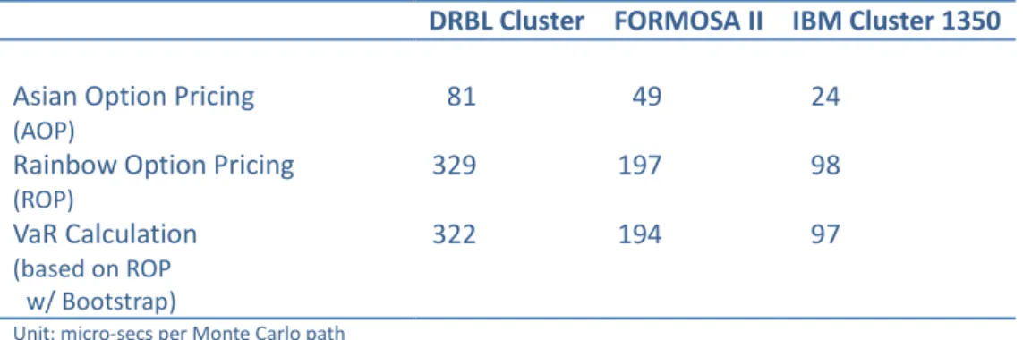
Table 1 Comparison of performance between DRBL-based PC platform with 32 nodes, FORMOSA II of NCHC with a batch job of 32 nodes and IBM Cluster 1350 with a batch job of 32 nodes. The PCs
are 20 XEON 2.6 GHz and 4GB RAM. ………... 29
Table 2 Comparison of Speedup ratios based on the calculations in Table 1. ………... 29 Table 3 Comparison of performance between Group A, which consists of
13 nodes from NCHC and 15 from UCSD, and Group B, which consists of 122 nodes collectively from UCSD, AIST, NCHC and Osaka University. The details of resources are referred to
(http://pragma-goc.rocksclusters.org/pragma-doc/resources.html). ………... 30 Table 4 Comparison of Speedup ratios based on the calculations in Table 3. ………... 31 Table 5 Summary of the case for the PC Grid calculations. ………... 32
vi
List of Figures
Figure 1 The trend history from Google Trend according to global Search Volume and global News Reference Volume, in which the alphabetic letters represent the specific events that relate to the each
curve. …... 2
Figure 2 Architecture of PicsouGrid for option pricing based on Monte
Carlo simulation (Stokes-Rees, 2007). …... 9 Figure 3 The architecture of Financial Information Grid (FinGrid). …... 9 Figure 4 Architecture of Integrated Risk Management System (Tanaka,
2003). …...10
Figure 5 The Semantic Discovery for Grid Services architecture (SEDI4G)
(Bell and Ludwig, 2005). …...11
Figure 6 RBNB DataTurbine use-scenario for collaborative applications. …...13 Figure 7 Pseudo random number plot comparing with quasi-random number
of Sobol for dimensions 1 and 2. …...23
Figure 8 Comparison of adjacent dimensions in Quasi-random number Sobol sequence. The dimensions are chosen according to prime numbers. There are high discrepancy found in higher dimensions of
Sobol sequence modified by Joe and Kuo (2003). …...24 Figure 9 Comparison of non adjacent dimensions. High discrepancy is
found in their correlations and forms clusters of islands in the
distribution. …...24
Figure 10 The distribution of probability in directional vector 𝑣𝑖,𝑗 of Sobol
sequences at i=3000 with j∈ {1, ⋯ ,1000} . The mean of the distribution is 0.491357, which approaches the mean of the normal
distribution 0.5. …...24
Figure 11 The convergence history of the mean value of Asian option pricing with risk-free interest rate r=0.1, underlying asset spot price S =100, strike price X=100, duration to maturity T=1 and volatility σ =0.3: The comparison is based on a single dimension of the extended high-dimensional Sobol sequences. The quasi random number generator (RNG) outperforms pseudo random number generator. The test also is conducted to compare the convergence history between different dimensions in Sobol sequences and found all perform consistently as shown in the right figure, in which the
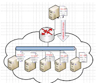
low dimension and high dimension are chosen for the comparison. …...25 Figure 12 The schematic of DRBL system: DRBL duplicates image files of
operational system via network to the clients, in which the clients’ original operational systems are untouched. Therefore, the clients are temporarily turned into dedicated compute resources, which
also provides additional security to financial data. …...28 Figure 13 Software stack developed in the PRAGMA grid. …...30 Figure 14 The architecture of Korea@Home, a specific @Home style PC …...32
vii
Grid used in our case study (Jun-Weon Yoon, 2008).
Figure 15 RBNB DataTurbine streaming open for data channels of iShares MSCI Taiwan Index (ETF) and TSEC weighted index from May 31, 2005 to May 31, 2008, and 30 days tick-by-tick trading data from Taiwan Futures Exchange Center (TAIFEX). (real data plot
viii
Nomenclature
c: Confidence level
P∶ Cumulative distribution function L∶ Large losses (or large negative returns) τ: Time horizon
X: Return
K: Strike price
T: Time to maturity of a derivative 𝑆𝑡: Asset price at t
r: Risk-free interest rate μ : Drift rate of an asset
σ:
Volatility of asset price V : Option value𝑥𝑖: Observed return value
F: Probability distribution
θ: Parameter of of a probability distribution 𝑉𝑑: 𝑑 × 𝑑 binary matrix
𝑁: Number of sampled points
B: Subcube
d: Dimension of a hypercube I: Value of Integral
𝐼 : Value of discrete integral
𝑞𝑛: Low discrepancy sequence with dummy index n
𝐷𝑁∗: Discrepany over a point set N.
𝑣𝑑: 𝑣𝑖,𝑗
d -dimensional Lebesgue measure
Direction number of Sobol sequence at ith step and jth dimension. W : Standard Wiener Process
Z: Random number
- 1 -
Chapter 1
Introduction
1.1 The Morale
In early year of 2006, Taiwan’s futures market revealed an interesting message that a foreign futures company Optiver Taiwan Co., Ltd, who was just open in July 2005, has monthly earnings nearly exceed that of Polaris MF Global Futures co Ltd a domestic leader in the futures market. Yet, Optiver Taiwan has just a few staffs and a computer system in its inception of operation. One may be curious and like to interrogate where its competitiveness comes from. The answer is now better understood that Optiver Taiwan got quicker response from their underlying computer system. The question may be raised if faster silos mean quicker response.
Indeed, securities trading is one of the few business activities where a few seconds processing delay can cost a company big fortune. The growing competitive in the market exacerbates the situation and pushes further towards instantaneous trading even in split second. The key obviously lies in the performance of the underlying information system. Rather than straight-through processes, which are considered as utopian Challenge of Wall Street firms, competitive advantage may come from three components for such a system: the tailored high performance financial analysis, seamless workflow and customized processes through the information systems.
1.2 Competitiveness through IT Performance
Following the computing evolution in financial services, it was a centralized process to begin with and gradually decentralized into a distribution of practical trading application logic across service networks. Financial services have tradition of doing most of its heavy lifting financial analysis in overnight batch cycles. However, in securities trading it cannot satisfy the need due to its ad hoc nature and requirement of immediate response.
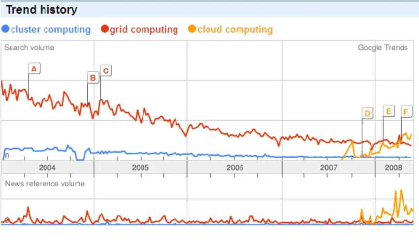
A new computing paradigm, Grid computing was emerged in the last decade. It was incorporated into the core context of a well referenced Atkins’ report of National Science Board of US, namely “Revolutionizing Science and Engineering Through Cyberinfrastructure‖ (Atkins et al, 2003), which lays down a visionary path for future IT platform development of the world. One may to observe this trend from statistics from Google Trend regarding the global Search Volume and global News Reference Volume of key phrases of ―Cluster Computing‖, ―Grid Computing‖ and ―Cloud Computing‖ (Fig. 1), which represents three main stream computing paradigms in high end quantitative analysis.
Cluster Computing is a group of coupled computers that work closely together so that in many respects they can be viewed as though they are a single computer. They are connected with high speed local area networks and the purpose is usually to gain more compute cycles with better cost
- 2 -
performance and higher availability. The Grid Computing aims at virtualizing scalable
geographically distributed computing and observatory resources to maximize compute cycles and data transaction rates with minimum cost. Cloud Computing is more of recent development owing to the similar technology used in global information services providers, such as Google, Amazon … etc. The Cloud is referred to as a subset of internet if to be explained in a simplest fashion. Within the cloud the computers also talk with servers instead of communicating with each other similarly to that of Peer to Peer Computing (Milojicic et al, 2002). There are no definitive definitions for the above terminology. However, people tend to view Clusters as one of foundational components of Grids, or Grids as a cluster of clusters on wide area networks. This is also known as horizontal integration. The Cloud provides an interface between users and Grids. This perspective considers Grids as a backbone of Cyberinfrastructure to support the Clouds. Similarly, in early days of development of Grids there is a so called ―@HOME‖ style PC Grids (Korpela et al, 2001), which are exactly working on at least ten of thousands of PCs, in which owners of PCs donate their CPU times when their machines are in idle. The PC Grids can be specifically categorized as Clouds.
Fig. 1 shows that there is a gradually drop in the curve of search volume for Grid Computing and Cluster Computing, and many surges and constant grows for Cloud Computing since its introduction in mid-2007. The size of the search volume strongly relates to the degree of maturity of each
computing paradigm. This is obvious in cluster computing. Clusters are the major market products, either in supercomputers from big vendors, such as IBM, HP, SGI and NEC…etc, or from
aggregation of PCs in university research laboratories. Fig. 1 also implies constant market need for high end computing. The General definition, which encompasses the Cluster Computing and the Cloud Computing, is adopted in this work.
Figure 1 The trend history from Google Trend according to global Search Volume and global News Reference Volume, in which the alphabetic letters represent the specific events that relate to each curve.
Grid computing is well suited to the challenge posed by the capital markets practices. Grid computing has been gaining popularity to serve as a production environment for finance services in
- 3 -
recent years. In this study the core computing competence for financial services will examined and how underlying algorithms for financial analysis can take advantage of Grids scrutinized. One of the most popular practiced algorithms is Monte Carlo Simulation (MCS) and it will be specifically used in our cases study for calculations of option pricing and for value at risk (VaR) in risk management.
Three grid platforms are carefully chosen to exploit the performance issue for financial services. The first one is traditional grid platform with heterogeneous and distributed resources. Usually digital packets are connected via optical fibers. For long distance, depending on network traffics, it will produce approximately 150~300 microseconds (mm) latency across Pacific Ocean. This is the physical constrain of light speed when traveling through the fiber channels. Therefore, even in split second packets can still travel to anywhere in the world. The Pacific Rim Applications and Grid Middleware Assembly (PRAGMA) grid is a typical example, which linked with 14 countries and 36 sites. The system is highly heterogeneous. The computer nodes mounted to PRAGMA grid range from usual PC clusters to high-end supercomputers. The second one is a special Linux, or DRBL, PC cluster. It converts system into a homogenous Linux system and exploits the compute cycles of the cluster. The intention is to provide dynamic and flexible resources to cope better with uncertainty of the traders’ cycle demand. Finally, PC grid is chosen to demonstrate finance services that can be effectively conducted through a Cloud-based computing. The usefulness of PC Grid is based on the fact that 90% of CPUs time of PCs were in idled status.
1.3 Organization
The following chapters are arranged as the following: In Chapter 2 Grid technology and Financial Services will be introduced in more details separately and then a study of financial services based on Grids given. In Chapter 3 Numerical methods that will be used in computational finance and the problem in migrating IT systems to Grids are introduced, in which Monte Carlo Simulation is specifically chosen to take advantage of the Grids and option pricing and value at risk are used as examples. Various grid platforms are also discussed. Three platforms are deliberately chosen for the calculation of option pricing and value at risk to demonstrate what Grids can do in Chapter 4. Finally this study is concluded in Chapter 5.
- 4 -
Chapter 2
Grid Technology for Financial Services
2.1 Information Technology (IT) and Financial Services
The finance industry involves a broad range of organizations that deal with the management of money. Among these organizations are banks, credit card companies, insurance companies, consumer finance companies, stock brokerages, investment funds and some government sponsored enterprises. The financial services industry represented 22.7% of the global market share in 2005 according to Gartner. In such a scale of market size, evidences found in IT impacts on financial services cannot be ignored.
The structure of the industry has changed significantly in the last two decades as companies, which are not traditionally viewed as financial service providers, have taken advantage of
opportunities created by technology to enter the market. New technology-based services have kept emerging. These changes are the result of the interaction of technology with other forces such as overall economic conditions, societal pressures, and the legal/regulatory environment in which the financial service industry operates. The effects of IT on the internal operations, the structure and the types of services offered by the financial service industry have been particularly profound (Phillips et al, 1984; Hauswald and Marquez, 2003; Griffiths and Remenyi, 2003). IT technology has been and continues to be both a motivator and facilitator of change in the financial service industry, which ultimately leads to competitiveness of the industry. The change is in particular radical after 1991 when World Wide Web was invented by Tim Berners-Lee and his group for information sharing in the community of high energy physics. It was later introduced to the rest of the world, which subsequently changed the face of how people doing business today.
Informational considerations have long been recognized to determine not only the degree of competition but also the pricing and profitability of financial services and instruments. Recent technological progress has dramatically affected the production and availability of information, thereby changing the nature of competition in such information sensitive markets. Hauswald and Marquez (2003) investigate how advances in information technology (IT) affect competition in the financial services industry, particularly credit, insurance, and securities markets. Two aspects of improvement in IT are focused: better processing and easier dissemination of information. In other words, two dimensions of technology progress that affects competition in financial services can be defined as advances in the ability to process and evaluate information, and in the ease of obtaining information generated by competitors. While better technology may result in improved information processing, it might also lead to low-cost or even free access to information through, for example, informational spillovers. They show that in the context of credit screening better
- 5 -
access to information decreases interest rates and the returns from screening. On the other hand, an improved ability to process information increases interest rates and bank profits. Hence
predictions regarding financial claims' pricing hinge on the overall effect ascribed to technological progress. Their results conclude that in general financial markets informational asymmetries drive profitability.
The viewpoint of Hauswald and Marquez is adopted in this study. Assuming competitors in the dynamics of financial market possess similar capacity, the informational asymmetries can be created sometimes only between seconds and now are possible to be achieved through the
outperformance of underlying IT platforms. This exactly reflects what is happening in the case of Optiver Taiwan mentioned earlier in Chapter 1. In the follow sections what advance of Grid technology can offer will be further discussed
2.2 Grid Technology 2.2.1 Definition of Grid
Grid was coined by Ian Foster (Foster and Kessleman, 2004) who gave the essence of the definitions as quoted below
“The sharing that we are concerned with is not primarily file exchange but rather direct access to computers, software, data, and other resources, as is required by a range of collaborative problem solving and resource-brokering strategies emerging in industry, science, and engineering. This sharing is, necessarily, highly controlled, with resource providers and consumers defining clearly and carefully just what is shared, who is allowed to share, and the conditions under which sharing occurs. A set of individuals and/or institutions defined by such sharing rules form what we call a virtual organization.‖
The definition is centered on the concept of virtual organization, but it is too conceptual to explain what the grid is. Foster then provides additional checklist as below to safeguard the possible logic pitfalls of the definition: Grid is a system that:
1) coordinates resources that are not subject to centralized control
A Grid integrates and coordinates resources and users that live within different control domains—for example, the user’s desktop vs. central computing; different administrative units of the same company; or different companies; and addresses the issues of security, policy, payment, membership, and so forth that arise in these settings. Otherwise, we are dealing with a local management system.
2) using standard, open, general-purpose protocols and interfaces
- 6 -
issues as authentication, authorization, resource discovery, and resource access. As discussed further below, it is important that these protocols and interfaces be standard and open. Otherwise, we are dealing with an application specific system.
3) to deliver nontrivial qualities of service.
A Grid allows its constituent resources to be used in a coordinated fashion to deliver various qualities of service, relating for example to response time, throughput, availability, and security, and/or co-allocation of multiple resource types to meet complex user demands, so that the utility of the combined system is significantly greater than that of the sum of its parts.
The definition of Grid thus far is well accepted and has been stably used up to now. The virtual organization (VO) has strong implication of community driven and collaborative sharing of distributed resources. The advance of development of optical fiber network in recent years plays a critical role of why Grids can be a reality. It is also the reason why now the computing paradigm shift to distributed/Grid computing.
Additionally, perhaps the most generally useful definition is that a grid consists of shared heterogeneous computing and data resources networked across administrative boundaries. Given such a definition, a grid can be thought of as both an access method and a platform, with grid middleware being the critical software that enables grid operation and ease-of-use. The above and more details of the primer of Grid are referred to Foster and Kessleman (2004).
2.2.2 Essence of Grid Technology
To realize the above goal, it needs to handle technically inter-operability of middleware
that is capable of communicating between heterogeneous computer systems across institutional boundaries. The movement of Grid began in 1996 by Ian Foster and Kessleman (2004). Before their development, another branch of high performance computing that focuses on connecting geographically distributed supercomputers to achieve one single grand task had been developed by Smarr and Catlett (1992). They coined such a methodology as metacomputing and their query has been how can we have infinite computing power under the physical limit, such as Moore’s Law. However, it remains to be less useful because its limit goal on pursuing top performance without noticing practical use in real world. The idea lives on and generates many tools dedicated to high performance/throughput computing, such as Condor (Litzkow, Livny and Mutka, 1988), Legion(Grimshaw and Wulf, 1997) and UNICORE (Almond and Snelling, 1999). Condor, as suggested by the name of the project, is devised to scavenge a large clusters of idle workstations. Legion is closer to the development of world-wide virtual computer. The goal of UNICORE is even much simpler and practical. It was developed due to Germany government decided to consolidate their 5 national supercomputer centers into a virtual one to reduce the management cost, and need a software tool to integrate them, hence the UNICORE. These tools were
- 7 -
successful under their development scope. However they fail to meet the first and the second items in Foster’s checklist in the previous section.
The emergency of Grids follows the similar path as that of Condor and Legion at the first place, which development aims at resources sharing in high performance computing. However, its vision in open standards and the concept of virtual organization allows its development go far beyond merely cluster supercomputers together. It gives a broader view of resources sharing, in which it is not only limited to the sizable computing cycles and storage space to be shared, but also extended virtually to calculable machines that are able to hook up to the internet, such as sensors and sensor loggers, storage servers, computers etc. Since 1996, Foster and his team have been developing software tools to achieve the purpose. Their software Globus Toolkit (Foster and Kessleman, 2004) is now a de facto middleware for Grids. However, the ambitious development is still considered insufficient to meet the ever growing complexity of grid systems.
As mentioned earlier that grid based on open specifications and standards, they allow all stakeholders within the virtual organization/grid to communicate with each other with ease and enable ones more to focus on integrated value creation activities. The open specifications and standards are made by the community of Open Grid Forum (OGF), which plays as a standard body and made, discussed and announced new standards during regular OGF meetings. Grid Specifications and Standards include Architecture, Scheduling, Resource Management, System Configuration, Data, Data movement, Security, Grid Security infrastructure. In 2004, OGF announced Globus Toolkit version, which adopt both the open standard of grid, Open Grid Services Architecture (OGSA), and the more widely adopted World Wide Web standard, Web services resrouce framework (WSRF), which ultimately enable grids to tackle issues of both scalability and complexity of very large grid systems.
- 8 -
2.3 Performance Enhancement via Grids
In this section two types of Grid systems, compute intensive and data intensive
respectively, are introduced. The classification of the types is based on various grid applications. Traditionally, the grid systems provides a general platform to harvest, or to scavenge if used only in idle status, compute cycles for a collection of resources across boundaries of institutional administration. In real world most applications are in fact data-centric. For example in a trading center, it collects tick-by-tick volume data from all related financial markets and is driven by informational flows, hence typical data-centric. However, as noted in Section 2.1 the core competence still lies on the performance enhancement of the IT system. The following two
subsections are will gives more details of compute intensive as well as data intensive grid systems by a survey of current development of Grids specifically for financial services. In some cases, e.g. high frequency data with real time analysis, two systems have to work together to get better performance. Our emphasis will be more on compute intensive grid system.
2.3.1 Compute Intensive Grid Systems
The recent development of computational finance based on grids is hereby scrutinized and remarks given. Our major interest is to see if the split second performance is well justified under the grid architecture. Also, real time issue with real market parametric data should be used as input for practical simulation. In addition, issues of inter-system, inter-disciplinary, geographically distribution of resources and the degree of virtualization are crucial to the success of such a grid. The chosen projects are reviewed and discussed as follow:
1.) PicsouGrid: This is a French Grid Project for Financial Service. It provides a general framework for computation Finance and targets on applications of options trading, options pricing, Monte Carlo simulation, aggregation of statistics etc (Stokes-Rees et al, 2007). The key for this development is the implementation of the middleware ProActive. ProActive is an in-house Java library for distributed computing developed by INRIA Sophia Antipolis, France. It provides transparent asynchronous distributed method calls and is implemented on top of Java RMI. It is also used in commercial applications. It also provides fault tolerance mechanism. The architecture is shown in Figure, which is very similar to most of grid applications apart from the software stack used. The option pricing was tested in an approximately 894 CPUs. The underlying computer systems are
heterogeneous. The system is used for metacomputing. As a result, the system has to specifically design to orchestrate and to synchronize and re-synchronize the whole distributed processes for one calculation. Once the grid system require synchronization between processes, which imply stronger coupling of algorithm of interest, the
performance will be seriously affected. There is no software treatment to solve such problems and should be tackled by physical infrastructure, e.g. optical fiber network with
- 9 -
Layer 2 light path.
Figure 2 Architecture of PicsouGrid for option pricing based on Monte Carlo simulation (Stokes-Rees, 2007).
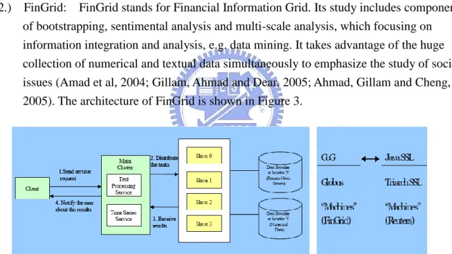
2.) FinGrid: FinGrid stands for Financial Information Grid. Its study includes components of bootstrapping, sentimental analysis and multi-scale analysis, which focusing on information integration and analysis, e.g. data mining. It takes advantage of the huge collection of numerical and textual data simultaneously to emphasize the study of societal issues (Amad et al, 2004; Gillam, Ahmad and Dear, 2005; Ahmad, Gillam and Cheng, 2005). The architecture of FinGrid is shown in Figure 3.
Figure 3 The architecture of Financial Information Grid (FinGrid).
It is a typical 3 tiers system, in which the first tier facilitates the client in sending a
request to one of the services: Text Processing Service or Time Series Service; the second tier facilitates the execution of parallel tasks in the main cluster and is distributed to a set of slave machines (nodes) and the third tier comprises the connection of the slave
machines to the data providers. This work focuses on small scale and dedicated grid system. It pumps in real and live numerical and textual data from say Reuters and performs real time sophisticated data mining analysis. This is a good prototype for
- 10 -
Finanical grid. However, it will encountered similar problem as that of PicsouGrid if it is to scale up. The model is more successful in automatically combining real data and the analysis.
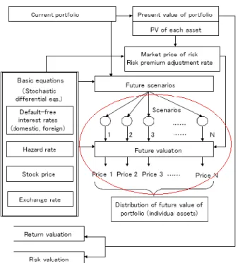
3.) IBM Japan collaborates with life insurance company and adopt PC grids concept to scavenge more compute cycles (Tanaka, 2003). In this work an integrated risk
management system (see Fig. 4) is modified, in which the future scenarios of red circle of Fig. 4 are send via Grid middleware to a cluster of PCs. According to the size of the given PCs, the number scenarios are then divided in a work balanced manner for each PC. This is the most typical use of compute intensive grid systems and a good practice for production system. However, the key issues that discussed in the above two cases cannot be answered in this study. Similar architecture can also be found in EGrid (Leto et al, 2005).
Figure 4 Architecture of Integrated Risk Management System (Tanaka, S. 2003).
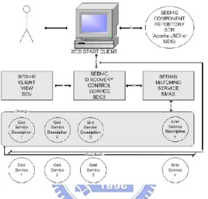
4.) UK e-Science developed a grid service discovery in the financial markets sector focusing on integration of different knowledge flows (Bell and Ludwig, 2005). From application’s viewpoint, business and technical architecture of financial service
applications may be segmented by product, process or geographic concerns. Segmented inventories make inter silo re-use difficult. The service integration model is adopted and a loosely coupled inventory – containing differing explicit capability knowledge. Three use cases were specifically chosen in this work to explore the use of semantic searching:
- 11 -
Use-case 1 – Searching for trades executed with a particular counterparty
Use-case 2 – Valuing a portfolio of interest rate derivative products
Use-case 3 – Valuing an option based product
The use-cases were chosen to provide examples of three distinct patterns of use – aggregation, standard selection and multiple selection. The architecture (see Fig. 5) is bound specifically with the user-cases. The advantage for grid in this case is that it can be easily tailored into specific user need to integrate different applications, which is a crucial strength of using grid.
Figure 5 The Semantic Discovery for Grid Services architecture (SEDI4G) (Bell and Ludwig, 2005).
2.3.2 Data Intensive Grid Systems
Grid in Financial Services from the perspective of web Services towards Financial Services Industry. The perspective is more on transactional side. Once the bottleneck of compute cycle is solved, the data-centric nature will play the key role again. The knowledge flows back to the customized business logic should provide the best path for users to access the live data of interest. There is no strong focus of development on this data intensive grid system. Even in FinGrid (Amad et al, 2004) which claims in streaming live data for real time analysis, the data issue remains part of compute grids. However, the need for dynamic data management is obvious as mentioned in (Amad et al, 2004). Hereby, we like to introduce and implement a dynamic data management software Ring Buffer Network Bus (RBNB)
- 12 -
RBNB Dataturbine was used recently to support global environmental observatory network, which involves linking with ten of thousand of sensors and is able to obtain the observed data online. It meets grid/cyberinfrastructure (CI) requirements with regard to data acquisition, instrument management, and state-of-health monitoring including reliable data capture and transport, persistent monitoring of numerous data channels, automated
processing, event detection and analysis, integration across heterogeneous resources and systems, real-time tasking and remote operations and secure access to system resources. To that end, streaming data middleware provides the framework for application development and integration.
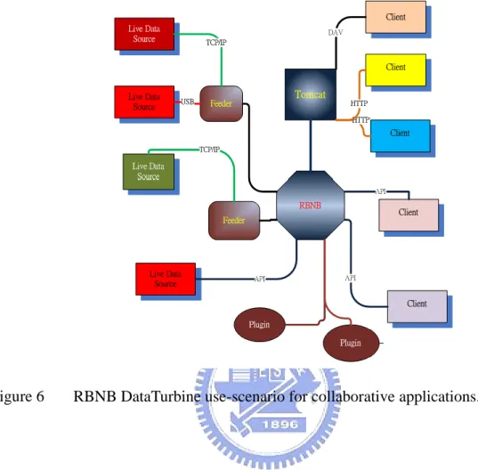
Use cases of RBNB Dataturbine include adaptive sampling rates, failure detection and correction, quality assurance and simple observation (see Tilak et al (2007)). Real-time data access can be used to generate interest and buy-in from various stakeholders. Real-time streaming data is a natural model for many applications in observing systems, in particular event detection and pattern recognition. Many of these applications involve filters over data values, or more generally, functions over sliding temporal windows. The RBNB DataTurbine middleware provides a modular, scalable, robust environment while providing security, configuration management, routing, and data archival services. The RBNB DataTurbine system acts as an intermediary between dissimilar data monitoring and analysis devices and applications. As shown in Figure 6 a modular architecture are used, in which a source
or ‖feeder‖ program is a Java application that acquires data from an external live data sources and feeds it into the RBNB server. Additional modules display and manipulate data fetched from the RBNB server. This allows flexible configuration where RBNB serves as a coupling between relatively simple and ‖single purpose‖ suppliers of data and consumers of data, both of which are presented a logical grouping of physical data sources. RBNB supports the modular addition of new sources and sinks with a clear separation of design, coding, and testing (ref. Figure 6). From the perspective of distributed systems, the RBNB DataTurbine is a ‖black box‖ from which applications and devices send data and receive data. RBNB
DataTurbine handles all data management operations between data sources and sinks, including reliable transport, routing, scheduling, and security. RBNB accomplishes this through the innovative use of memory and file-based ring buffers combined with flexible network objects. Ring buffers are a programmer-configurable mixture of memory and disk, allowing system tuning to meet application-dependent data management requirements. Network bus elements perform data stream multiplexing and routing. These elements
combine to support seamless real-time data archiving and distribution over existing local and wide area networks. Ring buffers also connect directly to client applications to provide streaming-related services including data stream subscription, capture, rewind, and replay.
- 13 -
This presents clients with a simple, uniform interface to real-time and historical (playback) data.
- 14 -
Chapter 3
Distributed and Parallel Financial Simulation
In the previous chapters, we address issues of incorporating IT technology for financial competitiveness and derive that the core lies on the performance of IT platform, providing the competitors in the market have similar capacity and equally informed. Grid technology, as the leading IT development in high performance computing, is introduced as the cutting edge IT platform to meet our goal. Many companies have adopted similar technology of Grids with
success as mentioned in Chapter 1. There are also increasing research interests, which result in the work discussed in Sec. 2.3. Better performance, however, cannot be achieved by merely using a single architecture as observed in the cases of Sec 2.3. The architecture obviously has to be specifically chosen for the analysis of interest. Simultaneously, the analysis procedures have to be tailored into the chosen architecture for performance fine tune.
In this chapter, we will introduce and discuss analysis procedures of financial simulation and how to tailor the analysis procedures into grid architectures by distribution and parallelism. The popular calculations for option pricing and for value at risk (VaR) in trading practice are used to serve the purpose. The calculation is based on Monte Carlo simulation, which is chosen not only because it is a well received approach due to the absence of straightforward closed form solutions for many financial models, but also a numerical method intrinsically suited to mass distribution and mass parallelism. The success of Monte Carlo simulation lies on the quality of random number generator, which will be discussed in details at the end of the chapter.
3.1 Financial Simulation
There are wide variety of sophisticated financial models developed, to name a few, ranging from analysis in time series, fractals, nonlinear dynamics and agent-based modeling to
applications in optional pricing, portfolio management and market risk measure etc (Schmidt, 2005), in which option pricing and VaR calculations of market risk measure can be considered crucial and one of the most practiced activities in market trading.
3.1.1 Option Pricing
An option is an agreement between two parties to buy or sell an asset at a certain time in the future for a certain price. There are two types of options:
Call Option: A call option is a contract that gives the right to its holder (i.e. buyer) without creating an obligation, to buy a pre-specified underlying asset at a predetermined price. Usually this right is created for a specific time period, e.g., six months, or more. If the option can be exercised only at its expiration (i.e. the underlying asset can be purchased only at the end of the
- 15 -
life of the option) the option is referred to as an European style Call Option (Or European Call). If it can be exercised any date before its maturity, the option is referred to as an American style Call Option (or American Call).
Put Option: A put option is a contract that gives its holder the right without creating the obligation, to sell a pre-specified underlying asset at a predetermined price. If the option can be exercised only at its expiration (i.e. the underlying asset can be sold only at the end of the life of the option) the option is referred to as a European style Put Option (Or European Put). If it can be exercised any date before its maturity, the option is referred to as an American style Put option (or American Put).
To price options in computational finance, we use the following notation: K is the strike price; T is the time to maturity of the option; 𝑆𝑡 is the stock price at time t; r is the risk-free interest rate; μ is the drift rate of the underlying asset (a measure of the average rate of growth of the asset price); σ is the volatility of the stock; V denotes the option value. Here is an example to illustrate the concept of option pricing. Suppose an investor enters into a call option contract to buy a stock at price K after three months. After three months, the stock price is 𝑆𝑡. If 𝑆𝑡 > 𝐾 then one can exercise one’s option by buying the stock at price 𝐾 and by immediately selling in the market to make a profit of 𝑆𝑇− 𝐾. On the other hand, If he 𝑆𝑇− 𝐾 to be buy the stock. Hence, we see a call option to buy the stock at time T at price K will get payoff 𝑆𝑇− 𝐾 + , where
𝑆𝑇− 𝐾 +≡ max( 𝑆
𝑇− 𝐾, 0) (Schmidt, 2005; Hull, 2003)
3.1.2 Market Risk Measurement based on VaR
Market risks are the prospect of financial losses , or gains, due to unexpected changes in market prices and rates. Evaluating the exposure to such risks is nowadays of primary concern to risk managers in financial institutions. Until late 1980s market risk were estimated through gap and duration analysis (interest rates), portfolio theory (securities), sensitivity analysis (derivatives) or scenarios analysis. However, all these methods either could be applied only to very specific assets or relied on subjective reasoning.
Since the early 1990s a commonly used market risk estimation methodology has been the Value at Risk (VaR). A VaR measure is the highest possible loss L incurred from holding the current portfolio over a certain period of time at a given confidence level (Dowd, 2002)
P 𝐿 > 𝑉𝑎𝑅 ≤ 1 − 𝑐 (3.1)
where 𝑐 is the confidence level, typically 95%, 97.5% or 99% and P is cumulative
distribution function. By convention, 𝐿 = −Δ𝑋(𝜏), where Δ𝑋(𝜏) is the relative change (return) in portfolio value over the time horizon 𝜏. Hence, large values of 𝐿 correspond to large losses (or
- 16 -
large negative returns).
The VaR figure has two important characteristics: 1) it provides a common consistent measure of risk across different positions and risk factors and 2) it takes into account the correlations or dependencies between different risk factors. Because of its intuitive appeal and simplicity, it is no surprise that in a few years Value at Risk has become the standard risk measure used around the world. However, VaR has a few deficiencies, among them the non-subadditivity – a sum of VaR’ s two portfolios can be smaller than the VaR of the combined portfolio. To cope with these
shortcomings, Artzner et al proposed an alternative measure that satisfies the assumptions of a coherent risk measure. The Expected Shortfall (ES), also called Expected Tail Loss (ETL) or Conditional VaR, is the expected value of the losses in excess of VaR:
ES = E 𝐿|𝐿 > 𝑉𝑎𝑅 (3.2)
It is interesting to note, that although new to the finance industry – Expected Shortfall has been familiar to insurance practitioners for a long time. It is very similar to the mean excess
function which is used to characterize claim size distribution, see(Cizek, Ha rdle and Weron, 2004) The essence of the VaR and ES computations is estimation of low quantiles in the
portfolio return distributions. Hence, the performance of market risk measurement methods depends on the quality of distribution assumptions on the underlying risk factors. Many of the concepts in theoretical and empirical finance developed over the past decades, including the classical portfolio theory, the Black-Scholes-Merton option pricing model and even the RiskMetrics variance-covariance approach to VaR rest upon the assumption that asset returns follow a normal distribution. The assumption is not justified by real market data. Our interest is more on the calculation side. For interested readers we refer further to (Weron, 2004).
3.2 Monte Carlo Simulations
3.2.1 Monte Carlo and Quasi-Monte Carlo Methods
In general, Monte Carlo (MC) and Quasi-Monte Carlo (QMC) methods are applied to estimate the integral of function 𝑓 𝑥 over 0,1 𝑑 unit hypercube where d is the dimension of the hypercube.
𝐼 = 𝑓 𝑥 𝑑𝑥
0,1 𝑑 (3.3)
In MC methods, I is estimated by evaluating 𝑓 𝑥 at N independent points randomly chosen from a uniform random distribution over 0,1 𝑑 and then evaluating average
- 17 - 𝐼 = 1 𝑁 𝑓 𝑥𝑖 𝑁 𝑖=1 (3.4)
From the law of large numbers, 𝐼 → 𝐼 as 𝑁 → ∞. The standard deviation is
1
𝑁 − 1 𝑓 𝑥𝑖 − 𝐼 2
𝑁
𝑖=1
(3.5)
Therefore, the error of MC methods is proportional to 𝑁−1/2.
QMC methods compute the above integral based on low-discrepancy (LD) sequences. The elements in a LD sequence are ―uniformly‖ chosen from 0,1 𝑑 rather than ―randomly‖. The discrepancy is a measure to evaluate the uniformity of points over 0,1 𝑑. Let 𝑞
𝑛 be a sequence
in 0,1 𝑑, the discrepancy 𝐷𝑁∗ of 𝑞𝑛 is defined as follows, using Niederreiter’s notation (Niederreiter, 1992). 𝐷𝑁∗ 𝑞 𝑛 = sup 𝐵 ∈ 0,1 𝑑 𝐴 𝐵, 𝑞𝑛 𝑁 − 𝑣𝑑 𝐵 (3.6)
Where B is a subcube of 0,1 𝑑 containing the origin, 𝐴 𝐵, 𝑞𝑛 is the number of points in 𝑞𝑛 that fall into B, and 𝑣𝑑 𝐵 is the d -dimensional Lebesgue measure of B. The elements of 𝑞𝑛
is said uniformly distributed if its discrepancy 𝐷𝑁∗ → 0 as 𝑁 → ∞. From the theory of uniform distribution sequences (Kuipers and Niederreiter, 1974), the estimate of the integral using a uniformly distributed sequence 𝑞𝑛 is 𝐼 =𝑁1 𝑁 𝑓 𝑞𝑛
𝑛=1 , 𝑎𝑠 𝑁 → ∞ then 𝐼 → 𝐼. The
integration error bound is given by the Koksman-Hlawka inequality:
𝐼 − 1 𝑁 𝑓 𝑞𝑛 𝑁 𝑛=1 ≤ 𝑉(𝑓) 𝐷𝑁∗ 𝑞 𝑛 (3.7)
where 𝑉(𝑓) is the variation of the function in the sense of Hardy and Krause (see Kuipers and Niederreiter, 1974), which is assumed to be finite.
The inequality suggests a smaller error can be obtained by using sequences with smaller discrepancy. The discrepancy of many uniformly distributed sequences satisfies 𝛰((log𝑁)𝑑/𝑁). These sequences are called lowdiscrepancy (LD) sequences (Chen, Thulasiraman and Thulasiram, 2006) . Inequality (3.7) shows that the estimates using a LD sequence satisfy the deterministic
- 18 -
error bound 𝛰((log𝑁)𝑑/𝑁).
3.2.2 Monte Carlo Simulations for Option Pricing
Under the risk-neutral measure, the price of a fairly valued European call option is the expectation of the payoff 𝐸 𝑒−𝑟𝑇 𝑆𝑇− 𝐾 + . In order to compute the expectation, Black and
Scholes (1973) modeled the stochastic process generating the price of a non-dividend-paying stock as geometric Brownian motion:
𝑑𝑆𝑡 = 𝜇𝑆𝑡𝑑𝑡 + 𝜎𝑆𝑡𝑑𝑊𝑡 (3.8)
where W is a standard Wiener Process, also known as Brownian motion. Under the risk-neutral measure, the drift 𝜇 is set to 𝜇 = 𝑟.
To simulate the path followed by S, suppose the life of the option has been divided into n short intervals of length Δ𝑡 Δ𝑡 = 𝑇/𝑛 , the updating of the stock price at t + Δ𝑡 from 𝑡 is (Hull, 2003):
𝑆𝑡+ Δ𝑡 − 𝑆𝑡 = 𝑟𝑆𝑡Δ𝑡 + 𝜎𝑆𝑡𝑍 Δ𝑡 (3.9)
Where 𝑍 is a standard random variable, i.e. 𝑍~ 0,1 . This enables the value of S Δt to be calculated from initial Value 𝑆𝑡 at time Δt, the value at time 2Δ𝑡 to be calculated from S Δt , and so on. Hence, a completed path for S has been constructed.
In practice, in order to avoid discretization errors, it is usual to simulate lnS rather than S. From Ito ’s lemma, the process followed by of (3.9) is (Bratley and Fox, 1988):
𝑑ln𝑆 = 𝑟 −𝜎2 2 𝑑𝑡 + 𝜎𝑑𝑧 (3.10) so that ln𝑆𝑡+ Δ𝑡− ln𝑆𝑡 = 𝑟 − 𝜎2 2 𝑑𝑡 + 𝜎𝑍 Δ𝑡 (3.11) or equivalently: 𝑆𝑡+ Δ𝑡 = 𝑆𝑡exp 𝑟 − 𝜎2 2 𝑑𝑡 + 𝜎𝑍 Δ𝑡 (3.12)
Substituting independent samples 𝑍𝑖, ⋯ , 𝑍𝑛 from the normal distribution into (3.12) yields independent samples 𝑆𝑇(𝑖), 𝑖 = 1, ⋯ , 𝑛, of the stock price at expiry time T. Hence, the option value is given by
- 19 - 𝑉 =1 𝑛 𝑉𝑖 = 1 𝑛 𝑛 𝑖=1 𝑒−𝑟𝑇 𝑛 𝑖=1 max 𝑆𝑇(𝑖)− 𝐾, 0 (3.13)
The QMC simulations follow the same steps as the MC simulations, except that the pseudo-random numbers are replaced by LD sequences. The basic LD sequences known in literature are Halton (1960), Sobol (1967) and Faure (1982). Niederreiter (1992) proposed a general principles of generating LD sequences. In finance, several examples have shown that the Sobol sequence is superior to others. For example, Galanti and Jung (1997) observed that ―the Sobol sequence outperforms the Faure sequence, and the Faure marginally outperforms the Halton sequence. In this research, we use Sobol sequence in our experiments. The generator used for generating the Sobol sequence comes from the modified algorithm 659 of Joe and Kuo (2003)
3.2.3 Monte Carlo Bootstrap for VaR
Monte Carlo simulation is applicable with virtually any model of changes in risk factors and any mechanism for determining a portfolio’s value in each market scenario. But revaluing a portfolio in each scenario can present a substantial computational burden, and this motivates research into ways of improving the efficiency of Monte Carlo methods for VaR.
The bootstrap (Efron 1981; Efron and Tibshirani, 1986) is a simple and straightforward method for calculating approximated biases, standard deviations, confidence intervals, and so forth, in almost any nonparametric estimation problem. Method is a key word here, since little is known about the bootstrap’s theoretical basis, except that (a) it is closely related to the jackknife in statistic inferring; (b) under reasonable condition it gives asymptotically correct results; and (c) for some simple problems which can be analyzed completely, for example, ordinary linear
regression, the bootstrap automatically produces standard solutions.
The bootstrap method is straightforward. Suppose we observe returns 𝑋𝑖 = 𝑥𝑖, 𝑖 = 1,2, ⋯ , 𝑛,
where the 𝑋𝑖 are independent and identically distributed (iid) according to some unknown
probability distribution F. The 𝑋𝑖 may be real valued, two-dimensional, or take values in a more
complicated space. A given parameter θ 𝐹 , perhaps the mean, median, correlation, and so forth, is to be estimated, and we agree to use the estimate θ = θ 𝐹 , where 𝐹 is the empirical
distribution function putting mass 1/n at each observed value 𝑥𝑖. We wish to assign some measure
of accuracy to θ .
Let σ 𝐹 be some measure of accuracy that we would use if F were known, for
example σ 𝐹 = SD𝐹 θ , the standard deviation of θ when 𝑋1, 𝑋2, ⋯ , 𝑋𝑛 ~𝐹 idd . The bootstrap
estimate of accuracy is σ = σ 𝐹 is the nonparametric maximum likelikhood estimate of σ 𝐹 . In order to calculate σ it is usually necessary to employ numerical methods. (a) A bootstrap sample 𝑋1∗, 𝑋2∗, ⋯ , 𝑋𝑛∗ is drawn from 𝐹 , in which each 𝑋𝑖∗ independently takes value 𝑥𝑗 with
- 20 -
probability 1/n, 𝑗 = 1,2, ⋯ , 𝑛. In other words, 𝑋1∗, 𝑋2∗, ⋯ , 𝑋𝑛∗ is an independent sample of size n
drawn with replacement from the set of observations 𝑥1, 𝑥2, ⋯ , 𝑥𝑛 . (b) This gives a bootstrap
empirical distribution function 𝐹 ∗, the empirical distribution of the n values 𝑋1∗, 𝑋2∗, ⋯ , 𝑋𝑛∗, and a
corresponding bootstrap value θ ∗ = θ 𝐹 ∗ . (c) Steps (a) and (b) are repeated, independently, a large number of times, say N, giving bootstrap values 𝜃 ∗1, 𝜃 ∗2, ⋯ , 𝜃 ∗𝑁. (d) The value of σ is approximated, in the case where σ 𝐹 is the standard deviation by the sample standard deviation of the 𝜃 ∗ values, where
𝜇 = 𝜃 ∗𝑗 𝑛 𝑗 =1 𝑁 (3.14) And 𝜎 2 = 𝜃 ∗𝑗 − 𝜇 2 𝑛 𝑗 =1 𝑁 − 1 (3.15)
3.3 Distribution and Parallelism based on Random Number Generation
Financial variables, such as prices and returns, are random time dependent variables. Wiener process plays the central role in modeling. As shown in (3.8) and (3.9) for approximating the underlying prices 𝑆𝑡+Δ𝑡, or the bootstrap samples of return 𝑋𝑖∗, The solution methods involve basic market parameters, drift 𝜇, volatility 𝜎 and risk-free interest rate r, current underlying price S or return 𝑋, strike price K, and Wiener process, which is related to time to maturity Δt and standard random variable 𝑍, i.e. ΔW = Z Δt. Monte Carlo methods simulate this nature of the Brownian motion directly. It follows Wiener process and approximates the standard random variable 𝑍 by introducing pseudo iid random number into each Wiener process. When the simulation number is large enough, e.g. if n in (3.13) is large enough, the mean value will
approach the exact solution. The large number for n also implies the performance problems are the key problems for Monte Carlo methods. One the other hand, the iid property of the random
number 𝑍 shows possible solution to tackle the performance problem through mass distribution and/or parallelism. The solution method centers on the random number generation.
The techniques of random number generation can be developed in a simple form through the approximation of a d-dimensional integral, e.g. (3.3). Mass distribution and parallelism required solutions of for large dimension. However, most modern techniques in random number generation have limitations. In this study, both tradition pseudo random number generation and high
dimensional low discrepancy random number generator are considered.
Following Section 3.2.1 better solution can be achieved by making use of Sobol sequences, which were proposed by Sobol (1967). A computer implementation in Fortran 77 was subsequently given by Bratley and Fox (1988) as Algorithm 659. Other implementations are available as C,
- 21 -
Fortran 77, or Fortran 90 routines in the popular Numerical Recipes collection of software. However, as given, all these implementations have a fairly heavy restriction on the maximum value of d allowed. For Algorithm 659, Sobol sequences may be generated to approximate integrals in up to 40 dimensions, while the Numerical Recipes routines allow the generation of Sobol sequences to approximate integrals in up to six dimensions only. The FinDer software of Paskov and Traub (1995) provides an implementation of Sobol sequences up to 370 dimensions, but it is licensed software. As computers become more powerful, there is an expectation that it should be possible to approximate integrals in higher and higher dimensions. Integrals in hundreds of variables arise in applications such as mathematical finance (e.g., see Paskov and Traub (1995)). Also, as new methods become available for these integrals, one might wish to compare these new methods with Sobol sequences. Thus, it would be desirable to extend these existing
implementations such as Algorithm 659 so they may be used for higher-dimensional integrals.We remark that Sobol sequences are now considered to be examples of (t, d)-sequences in base 2. The general theory of these low discrepancy (t, d)-sequences in base b is discussed in detail in
Niederreiter (1992). The generation of Sobol sequences is clearly explained in Bratley and Fox (1988). We review the main points so as to show what extra data would be required to allow Algorithm 659 to generate Sobol sequences to approximate integrals in more than 40 dimensions. To generate the j th component of the points in a Sobol sequence, we need to choose a primitive polynomial of some degree sj in the field ℤ2 that is, a polynomial of the form
𝑥𝑠𝑗 + 𝑎1,𝑗𝑥𝑠𝑗−1 + ⋯ + 𝑎𝑠𝑗−1,𝑗𝑥 + 1, (3.16)
where the coefficients 𝑎1,𝑗,⋯ ,𝑎𝑠𝑗−1,𝑗 are either 0 or 1.
We use these coefficients to define a sequence 𝑚1,𝑗, 𝑚2,𝑗, ⋯ of positive integers by the recurrence relation 𝑚𝑘,𝑗 = 𝑎1,𝑗𝑚𝑘−1,𝑗⨁22𝑎 2,𝑗𝑚𝑘−2,𝑗⨁ ⋯ ⨁2𝑠𝑗−1𝑎 𝑠𝑗−1,𝑗𝑚𝑘−𝑠𝑗+1,𝑗⨁2 𝑠𝑗𝑎 𝑠𝑗,𝑗𝑚𝑘−𝑠𝑗,𝑗⨁𝑚𝑘−𝑠𝑗,𝑗 (3.17)
for 𝑘 ≥ 𝑠𝑗 + 1, where ⊕ is the bit-by-bit exclusive-OR operator. The initial values
𝑚1,𝑗, 𝑚2,𝑗, ⋯ , 𝑚𝑠𝑗,𝑗 can be chosen freely provided that each 𝑚𝑘,𝑗, 1 ≤ 𝑘 ≤ 𝑠𝑗 is odd and less than 2𝑘. The ―direction numbers‖ 𝑣1,𝑗, 𝑣2,𝑗, ⋯ are defined by
𝑣1,𝑗 ≡ 𝑚𝑘,𝑗 2𝑘
(3.18)
Then 𝑥𝑖,𝑗 , the j th component of the ith point in a Sobol sequence, is given by
- 22 -
where 𝑏𝑙is the lth bit from the right when i is written in binary, that is, ⋯ 𝑏2𝑏1 2 is the
binary representation of i. In practice, a more efficient Gray code implementation proposed by Antonov and Saleev (1979) is used; see Bratley and Fox (1988) for details. We then see that the implementation in Bratley and Fox (1988) may be used to generate Sobol sequences to
approximate integrals in more than 40 dimensions by providing more data in the form of primitive polynomials and direction numbers (or equivalently, values of 𝑚1,𝑗, 𝑚2,𝑗, ⋯ , 𝑚𝑠𝑗,𝑗). When
generating such Sobol sequences, we need to ensure that the primitive polynomials used to generate each component are different and that the initial values of the 𝑚𝑘,𝑗’s are chosen differently for any two primitive polynomials of the same degree. The error bounds for Sobol sequences given in Sobol (1967) indicate we should use primitive polynomials of as low a degree as possible. We discuss how additional primitive polynomials may be obtained in the next section. After these primitive polynomials have been found, we need to decide upon the initial values of the 𝑚𝑘,𝑗 for 1 ≤ 𝑘 ≤ 𝑠𝑗 . As explained above, all we require is that they be odd and that 𝑚𝑘,𝑗 < 2𝑘. Thus, we could just choose them randomly, subject to these two constraints. However, Sobol (1988) introduced an extra uniformity condition known as Property A. Geometrically, if the cube 0,1 𝑑 is divided up by the planes 𝑥
𝑗 = 1 ∕ 2 into 2𝑑 equally sized subcubes, then a
sequence of points belonging to 0,1 𝑑 possesses Property A if, after dividing the sequence into
consecutive blocks of 2𝑑points, each one of the points in any block belongs to a different subcube. Property A is not that useful to have for large d because of the computational time required to approximate an integral using 2𝑑 points. Also, PropertyA is not enough to ensure that there are no bad correlations between pairs of dimensions. Nevertheless, Property A would seem a reasonable criterion to use in deciding upon a choice of the initial 𝑚𝑘,𝑗 . The numerical results for Sobol sequences given in Section 4 suggest that the direction numbers obtained here are indeed reasonable. Sobol (1967) showed that a Sobol sequence used to approximate a d dimensional integral possesses Property A if and only if
det(𝑉𝑑) = 1 (mod 2), (3.20)
where 𝑉𝑑 is the d × d binary matrix defined by
𝑉𝑑 = 𝑣1,1,1 𝑣2,1,1 𝑣1,2,1 𝑣2,2,1 ⋯ 𝑣𝑑,1,1 𝑣𝑑,2,1 ⋮ ⋱ ⋮ 𝑣1,𝑑,1 𝑣2,𝑑,1 ⋯ 𝑣𝑑,𝑑,1 (3.21 )
with 𝑣𝑘,𝑗 ,1 denoting the first bit after the binary point of 𝑣𝑘,𝑗 . The primitive polynomials and direction numbers used in Algorithm 659 are taken from Sobol and Levitan (1976) and a subset of this data may be found in Sobol (1967). Though it is mentioned in Sobol (1967) that Property A is satisfied for 𝑑 ≤ 16, that is, det(𝑉𝑑) = 1 (mod 2) for all 𝑑 ≤ 16, our calculations
- 23 -
showed that Property A is actually satisfied for 𝑑 ≤ 16. As a result, we change the values of the 𝑚𝑘,𝑗 for 21 ≤ 𝑗 ≤ 40, but keep the primitive polynomials. For 𝑗 ≥ 41, we obtain additional primitive polynomials. The number of primitive polynomials of degree s is ϕ 2𝑠− 1 s ,
where ϕ is Euler’s totient function. Including the special case for 𝑗 = 1 when all the 𝑚𝑘,𝑗 are 1, this allows us to approximate integrals in up to dimension 𝑑 = 1111 if we use all the primitive polynomials of degree 13 or less. We then choose values of the 𝑚𝑘,𝑗 so that we can generate Sobol sequences satisfying Property A in dimensions d up to 1111. This is done by generating some values randomly, but these are subsequently modified so that the condition det(𝑉𝑑) = 1 (mod
2) is satisfied for all d up to 1111. This process involves evaluating values of the 𝑣𝑘,𝑗 ,1’s to obtain the matrix 𝑉𝑑 and then evaluating the determinant of 𝑉𝑑. A more detailed discussion of this strategy is given in the next section. It is not difficult to produce values to generate Sobol’s points for approximating integrals in even higher dimensions.
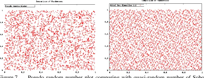
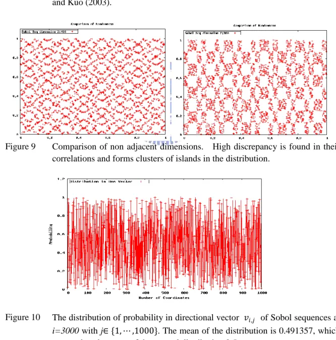
The following figures is the two dimensional plots of high dimension Sobol sequences of Joe and Kuo with 𝑑 = 1000. It is compared with pseudo random number generation. The number of sampling points is 3000. In Figure 7 pseudo random number is plotted in comparison with that of quasi-random number of Sobol. The leading dimensions 1 and 2 of Sobol sequences are used. The improvement is immense. In order to understand more of the nature of Sobol sequences, we chose prime dimensional numbers 499, 503, 991 and 997 respectively as suggested by Joe and Kuo. The results are plotted in Figure 8 and Figure 9. It is found that there are stronger
correlations between Sobol sequences of non-adjacent dimensions in the fashion of the
dimensional comparison of their randomness. Larger numbers of sampling points, e.g. 10,000, are also tested and the patterns persist. It implied the violation of idd assumption and may incur problems in mass distribution and parallelism, in which each process the random number is generated independently without knowing what other processes are doing. The dependency may deteriorate the quality of randomness. Nevertheless, in our numerical experiments there are no significant differences found thus far.
- 24 -
for dimensions 1 and 2.
Figure 8 Comparison of adjacent dimensions in Quasi-random number Sobol sequence. The dimensions are chosen according to prime numbers. There are high discrepancy found in higher dimensions of Sobol sequence modified by Joe and Kuo (2003).
Figure 9 Comparison of non adjacent dimensions. High discrepancy is found in their correlations and forms clusters of islands in the distribution.
Figure 10 The distribution of probability in directional vector 𝑣𝑖,𝑗 of Sobol sequences at i=3000 with j∈ {1, ⋯ ,1000}. The mean of the distribution is 0.491357, which approaches the mean of the normal distribution 0.5.
- 25 -
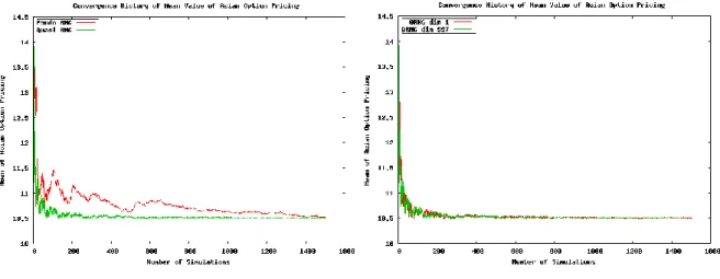
Figure 11 The convergence history of the mean value of Asian option pricing with risk-free interest rate r=0.1, underlying asset spot price S =100, strike price X=100, duration to maturity T=1 and volatility σ =0.3: The comparison is based on a single dimension of the extended high-dimensional Sobol sequences. The quasi random number generator (QRNG) outperforms pseudo random number generator. The test also is conducted to compare the convergence history between different dimensions in Sobol sequences and found all perform consistently as shown in the right figure, in which the low dimension and high dimension are chosen for the comparison.