行政院國家科學委員會專題研究計畫成果報告
應用 DSMC 法模擬分析深次微米銅化學氣相沈積之熱流場及沈積度 Using DSMC to Simulate Ther mal-flow Field on Deep Naro-Meter Trench for
Cu-CVD 計畫編號 NSC89-2212-E009-024 執行期限八十八年八月一日至八十九年七月三十一日 主持人:陳俊勳教授 交通大學機械系教授 摘要 本 計 畫 使 用 直 接 模 擬 蒙 地 卡 羅 法 (DSMC),分析鼓式曳引分子幫浦(MDP)的 簡化模型,以得到它的壓縮特性及傳輸機 率。文中主要在探討在不同的上板速度(正 比於轉子速度)、轉子凹槽的長寬比與背壓 值等條件下,對整個幫浦的抽氣效率之影 響,並與 Iguchi 等人[1]實驗所得的抽氣速 率曲線作趨勢性的比較。以往在預測最大 壓縮比的公式中,多假設與背壓的大小無 關,或在模擬時假設進出口的平均速度為 零,本文將針對上述的假設做改進,使模 擬更接近真實的情形。最後,所得的結果 分別與 Lee 等人[2]的模擬結果作比較,希 望對 MDP 的性能有更佳的預測結果。預測 結 果 顯 示 : 在 分 子 流 中 當 板 速 超 過 0.25VMP 時,在流體速度向量場中,於出 口端呈現渦流的情形,相關的 CFD 數值模 擬也有類似的現象產生;在自由分子流域 中,順著流體方向的傳輸機率,隨著上板 的速度增加而漸增,最後到達一個定值, 其值略小於 1;當轉子上凹槽的長寬比漸 增,傳輸機率並沒有明顯地改變,而幾近 一定值;此外,在過渡流域中,MDP 所呈 現的傳輸機率,於不同的背壓下呈現一定 值;隨著操作壓力的範圍不同,最大壓縮 比也有明顯地改變。最後,用改進的模型 分別與 Lee 等人的數值和 Iguchi 等人的實 驗曲線作比較,在趨勢上可得到不錯的一 致性。 關鍵詞:直接模擬蒙地卡羅法,分子曳引 式幫浦,傳輸機率,最大壓縮比 Abstr act
This project simulates the performance of transmission probability and compression characteristics for a simple drum type of molecular drag pump (MDP) model by using DSMC method. The modification of the present model is that the inlet and outlet bulk velocities are no longer null, but obtained by meeting the requirement of mass balance. The work aims at exploring the pumping
efficiency with various operating parameters, including the wall velocity, channel aspect ratio and backpressure. The predicted results are compared with the experimental data by Iguchi et al. [1] to verify them in qualities. In the past studies, the maximum compression ratio (Ko) is not affected by backpressure, or the mean bulk velocity at the MDP inlet and outlet are assumed zero. Therefore, the present work is motivated to relax these limitations to achieve a better prediction for MDP performances. Finally, the computed results are compared with those by Lee et al. [2]. The predicted results show that according to the velocity vector fields, a vortex at outlet is found as the wall velocity is greater than 0.25VMP at very rarefied condition which the similar phenomenon was observed by the related CFD numerical simulation. In free molecular regime, transmission probability in flow direction (Tr1) increases with an increase in wall speed (uwall), and it approaches a constant value, smaller than unity. The change in transmission probability (Tr1) is strongly dependent on the wall speed, but weakly dependent on the channel length. In the transition regime, the transmission probability can be thought to have nearly constant value irrespective of the backpressure (P2). The maximum compression ratio (Ko) is found to change significantly according to Kundsen number in the flow field. Finally, the predicted results by this model show a good agreement with the ones by Lee et al. and the experimental data by Iguchi et al..
Keywor ds: DSMC, MDP, Transmission
Probability, Maximum Compression Ratio
Introduction
The present study is to investigate the performance of a MDP (Fig. 1) in a simplified geometry, illustrated in Fig. 2, which was proposed by Lee et al. [2].
Before the last reference, the maximum compression ratio was estimated as a function of (uwall×L/H), where uwall is the wall velocity and L/H is the aspect ratio of the channel, in an exponential form. While the mean collision length from the wall is constant over the whole flow channel, this kind of estimation could be appropriate. However, the gas flow tends to be collimated as the channel length increases. Therefore, for long channel the beaming effect plays an important role, as indicated by Liu et al. [3]. In addition, the flow in the rear portion of drag stages becomes transitional or continuum due to the local high-pressure. The simulation results in reference 2 showed that the existing theories for estimating maximum compression ratio present the inaccurate solutions if the pressure variation in the channel is large. Furthermore, the transmission probability of the pumped gas molecules in flow direction has a nearly constant value no matter what the channel length and exhaust pressure are in normal operational conditions. However, a shortcoming of reference 2 is that they assume zero mean velocities at the MDP inlet and outlet, which is improper in reality, in the molecular and transition regimes. Therefore, the present work is motivated to relax this limitation by using a special treatment, developed by Wu [4], to obtain the accurate velocities at both channel ends. The other improvement is that the outlet temperature is not prescribed in advance, but provided as a part of solution. The main purpose is to achieve the better prediction of MDP performances.
Mathematical Model
In this project, the gas is assigned to flow in a simplified two-dimensional (2-D) channel, whose depth is H and channel length L, as shown in Fig. 2. The relative coordinate is attached on groove surface, therefore, the stator (cover) is moving at a speed, uwall, in the positive direction of x-axis. The flow field is simulated by using direct simulation Monte Carlo (DSMC) method over a wide range of pressure, covering the free molecular, transitional, and continuum regimes. The VHS, NTC, diffuse reflection, rotational energy and area cells schemes are adopted to deal with the 2-D problem. The simulated gas is N2. Modification of boundary conditions at inlet and outlet are:
Inlet condition
The total number flux from inlet to inlet boundary is ( ) [ ]
{
e s erf s}
n N s i = + + − 1 2 2 1 2 2 1 π β π.
The total molecules from inlet to inlet boundary per unit time is
i i
i N A
N&= ×
.
Inlet boundary condition
The total molecules per unit time from inlet boundary to inlet can be obtained in terms of the n1, and VMP1, which are gained by DSMC program inside the calculation domain. After a time step, the new velocity is known through i i i i A n N N U × − = & &1
.
Outlet conditionThe total number flux from outlet to outlet boundary is ( ) [ ]
{
e s erf s}
n N s o = + + − 1 2 2 1 2 2 1 π β π.
The total molecules from outlet to outlet boundary per unit time is
o o
o N A
N& = ×
.
Outlet boundary condition
The total molecules per unit time from outlet boundary to outlet can be obtained in terms of the n2, and VMP2, which are gained by DSMC program inside the calculation domain. After a time step, the new velocity is known through o o o o A n N N U × − = &2 &
.
This project adopts 15 simulated molecules per cell and the time step selected is based on the one-sixth mean collision time. The cell size in the y direction is based on the λh, which is the mean free path at high pressure end. In the x direction, the cell size is ranged from λh to 4λh according to the pressure and channel length.
Results and discussion
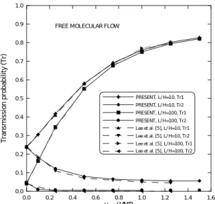
Fig. 3 shows the comparisons of Tr’s at inlet and outlet between the present study and reference 5 for free molecular flow (Knl = ∞)
with L/H=10 and 100. The ordinate is Tr and the abscissa is the ratio of the wall velocity to most probable thermal speed (uwall/VMP). In the case of L/H=10, the discrepancy between Tr1 and Tr2 for both studies is indistinguishable. When the wall is stationary, Tr1 and Tr2 are identical. As the wall velocity increases, Tr2 drops rapidly. The reason will be given in next paragraph. Once the wall velocity becomes higher than VMP, then, it approaches a constant value, which is much less than 1. For Tr1, it increases with an increase of uwall/VMP. Similar to Tr1, it tends to reach a constant value as uwall/VMP is greater than 1. When L/H=100, the tendency is completely the same as that of L/H=10. The most significant difference between these two cases occurs at the zero wall velocity. At that condition, it can be seen that Tr1 and Tr2 in the case of L/H=10 is higher than those of L/H=100. It is because that the probability for molecules to collide back becomes greater for the longer channel, leading to a lower Tr. However, as the wall velocity increases, Tr1 increases and it approaches a constant value, which is almost the same as the one in the case of L/H=10, irrespective of the channel length. For Tr2 in the case of L/H=100, its trend is similar to that of L/H=10, but its asymptotic value is lower, indicating that the value of Tr2 at high wall velocity is strongly dependent on the channel length.
The velocity vector fields as a function of wall velocity are shown in Fig. 4. The other parameters are kept as the same as those in reference case. When the wall velocity (uwall) is equal to 0.1VMP, the main stream is from right toward left, although the wall is moving in opposed direction. Apparently, the momentum gained from the moving wall can’t encounter the pressure gradient yet. However, flow velocities near the upper wall are smaller than the ones close to the bottom wall, because the pressure gradient effect is greatly balanced there by the momentum from the wall. Increasing uwall to 0.25 VMP, the velocity vectors in most area are toward inlet. However, around the high-pressure end (outlet), the flow near the moving wall is the same direction as that of wall, and a vortex is formed locally. This causes Tr2 to decrease. Of course, it indicates that the effect of moving wall becomes greater. When uwall increases to 0.5 VMP, the main stream direction now becomes coincident with the moving wall. The vortex moves
downward. The trend is maintained as the moving wall velocity increases and the size of vortex shrinks. The vortex is caused by that the momentum of molecules given by the moving wall can’t conquer the one provided by the opposed pressure gradient. With the same compression ratio, the vortex is expected to vanish when the channel becomes longer which makes the pressure gradient to decrease.
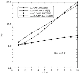
Fig. 5 demonstrates the effect of L/H on Ko for various wall velocity ratios under the specified Kn1=6.7. It reveals that Ko rises with increasing the channel length for both wall velocities equal to 0.2 and 1.0 VMP. In the present study, the Log(Ko) is linearly proportional to L/H approximately, therefore, Ko can be shown as a function of an exponential form of L/H. Apparently, the predicted results by using DSMC method confirm the expression of
) exp( H u L K wall o × = α
.
In Fig. 6, Kni is 67, which is much greater than the one in last figure. According to the above equation, both Ko’s in Figs. 5 and 6 would be the same, since both have the same uwall and L/H. However, Ko in this case is less than the corresponding one, especially in the high value of L/H. Apparently, Kni must play an important role for this discrepancy. The definition of Kn is λ/H. Since H is maintained as constant, Kn is directly proportional to λ, which strongly depends on local pressure, i.e. λ = 0.05/P at room temperature. Therefore, it can conclude that the pressure effect can not be ignored for the expression of Ko. When the collisions increase due to high pressure, it leads the gas molecules to have greater momentum in flow direction. In order to balance it, the backstreaming molecules must raise their pressure. This contributes to a higher Ko.
Reference
1. M. Iguchi, M. Nagakubo, S. Hashimoto, S. Kaneto, and H. Oikawa, “Development of New Molecular Pump (I),” Osaka Vacuum,
Ltd., Hachioji, Tokyo, Japan.
2. Y. K. Lee and J. W. Lee, “Direct simulation of compression characteristics for a simple drag pump model,” Vacuum,
47, pp. 807-809, 1996.
3. N. Liu, Y. Zhu, X. Z. Wang and S. J. Pang,
drag conditions,” J. Vac. Sci. Technol., A
9(6), p. 3159, 1991.
4. J. S. Wu, F. Lee, and S. C. Wong,
“Pressure boundary treatment in
micromechanical devices using direct simulation Monte Carlo method,” Oct,
1999.(Submitted for publication)
Fig. 1 Main structure of molecular drag pump
Fig. 2 The scheme of simulation boundaries, computing domain and net cells
Fig. 3 Effect of the wall velocity on the transmission probability of gas flow for free molecular condition (a) (b) (c) (d) (e)
Low pressure end
Inlet
High pressure end
Outlet
Upper wall (rotor) moving with velocity uwall
Lower wall rest (stator) X H L Y uwall direction P h , O u tle t 0.1 0.2 0.3 0.4 0.5 0.6 0.7 0.8 0.9 1.0 X (m) 0.1 Y (m ) 0.1 0.2 0.3 0.4 0.5 0.6 0.7 0.8 0.9 1.0 X (m) 0.1 Y (m ) 0.1 0.2 0.3 0.4 0.5 0.6 0.7 0.8 0.9 1.0 X (m) 0.1 Y (m ) 0.2 0.6 1.0 1.4 0.0 0.4 0.8 1.2 1.6 u / VMP 0.1 0.3 0.5 0.7 0.9 0.0 0.2 0.4 0.6 0.8 1.0 T ra n s m is s io n p ro b a b il it y (T r) PRESENT, L/ H=10, Tr1 PRESENT, L/ H=10, Tr2 PRESENT, L/ H=100, Tr1 PRESENT, L/ H=100, Tr2 Lee et al. [5], L/ H=10, Tr1 Lee et al. [5], L/ H=10, Tr2 Lee et al. [5], L/ H=100, Tr1 Lee et al. [5], L/ H=100, Tr2
FREE MOLECULAR FLOW
wall 0.0 0.1 0.2 0.3 0.4 0.5 0.6 0.7 0.8 0.9 X (m) 0.1 Y (m ), P l, In le t 0.0 0.1 0.2 0.3 0.4 0.5 0.6 0.7 0.8 0.9 X (m) 0.1 Y (m )
Fig. 4 The velocity vector fields with the upper wall velocity (uwall) are , (a) 0.1, (b) 0.25, (c) 0.5, (d)
0.75,and (e)1 VMP
Fig. 5 Effect of the inlet pressure on Ko for Kni=6.7
and various wall velocity ratios
Fig. 6 Effect of the inlet pressure on Ko for Kni=67
and various wall velocity ratios
1 3 5 7 9 0 2 4 6 8 10 L / H 0 1 10 100 K 0 Kni = 67 u =VMP, PRESENT u =VMP, Lee et al.[5] u =0.2VMP, PRESENT u =0.2VMP, Lee et al.[5] wall wall wall wall 1 3 5 7 9 0 2 4 6 8 10 L / H 0.1 1.0 10.0 100.0 K o Kni = 6.7 u =VMP, PRESENT u =VMP, Lee et al.[5] u =0.2VMP, PRESENT u =0.2VMP, Lee et al.[5] wall wall wall wall