指向性感測網路上有效確保時間性覆蓋之感測器佈署以及其物體監控之應用

(1)

國

立

交

通

大

學

資訊科學與工程研究所

碩

士

論

文

指向性感測網路上有效確保時間性覆蓋之

感測器佈署以及其物體監控之應用

Efficient Deployment Schemes of Rotatable, Directional

(R&D) Sensors to Achieve Temporal Coverage of Objects

and its Applications

研究生：陳勇甫

指導教授：曾煜棋教授

(2)

指

指向

向

向性

性

性感

感

感測

測

測網

網

網路

路

路上

上

上有

有效

有

效

效確

確

確保

保

保時

時

時間

間

間性

性

性覆

覆

覆蓋

蓋

之

之感

感

感測

測

測器

器

器佈

佈

佈署

署

署以

以

以及

及

及其

其

其物

物

物體

體

體監

監

監控

控

控之

之

之應

應

應用

用

學生：陳勇甫指導教授：曾煜棋教授國立交通大學資訊科學與工程研究所碩士班摘摘摘要要要於諸多無線感測器網路的應用中，由於應用需求或是設備限制，感測器之感測幅度為扇形範圍。此外，輔以器械的幫助，如步進馬達，這些感測器便可透過旋轉來覆蓋其周圍的目標物，這類型的感測器被稱為旋轉式指向性(R&D)感測器。在論文中，我們考慮R&D感測器的佈署問題，其決定如何放置最少數的R&D感測器，以符合覆 蓋特定物體的條件，如此每個目標物皆可為δ-time covered，其中0 < δ ≤ 1。若在一段 固定的周期時間T裡，目標物可被一個感測器覆蓋至少達到δT 時間，則可稱此目標物 為δ-time covered。R&D感測器的佈署問題是NP-hard，因此我們提出了兩個有效的探索 法，第一個方法為最大覆蓋佈署(MCD)演算法，其核心在於佈署感測器以覆蓋最多的目標物；第二個方法為圓盤重疊覆蓋佈署(DOD)演算法，利用處理感測器覆蓋範圍間的重疊問題，以降低感測器的數目。模擬實驗中，針對不同目標物分布情形可顯示出各方法的有效性。此外，為了實證本篇論文所提出的時間性覆蓋模型之特性，我們利用R&D感測器開發一個事件導向視覺監控系統，於此系統中，R&D感測器利用紅外線偵測與攝影機來定期地監測目標物，當目標物失竊時，偵測到的感測器會回報含有快照細節的警告訊息給使用者。關關關鍵鍵鍵字字字：：：指向性感測器，轉動，監測系統，時間性覆蓋，無線感測器網路。

(3)

Route-Aware Mobile Relay Deployment for

Traffic Redirection in a Wireless Ad Hoc Network

Student: Yung-Fu Chen Advisor: Prof. Yu-Chee Tseng Department of Computer Science

National Chiao Tung University ABSTRACT

In many wireless sensor applications, sensors may possess sector-like sensing coverage due to application requirements or equipment constraints. In addition, with the help of machinery such as stepper motors, these sensors can rotate to cover the objects around them. This type of sensor is called a rotatable, directional (R&D) sensor. In the paper, we consider the R&D sensor

deployment problem, which determines how to place the minimum number of R&D sensors to

cover a given set of objects, such that each object can be δ-time covered, where 0 < δ ≤ 1. In particular, an object is said to be δ-time covered if during a fixed period T , the object can be covered by one sensor for at least δT time. The R&D sensor deployment problem is NP-hard and we thus propose two efficient heuristics. The first heuristic, called the maximum covering

deployment (MCD) algorithm, always places sensors such that the maximum number of objects

can be covered. On the other hand, the second heuristic, called the disk-overlapping deployment

(DOD) algorithm, exploits the overlap between sensors’ coverage to save sensors. Simulation

results show the effectiveness of the proposed heuristics under different distributions of objects. Moreover, to demonstrate the feasibility of our temporal coverage model, we develop an

event-based visual surveillance system by R&D sensors. In this system, objects are periodically

monitored by R&D sensors equipped with infrared detectors and cameras. When one object is taken away, the monitoring sensor will report a warning message along with the detailed snapshots to the user.

Keywords: directional sensor, rotation, surveillance system, temporal coverage, wireless sensor network.

(4)

誌

謝

本篇論文是集結研究所兩年來學習之所成，有幸承蒙眾人之恩澤與扶持，使我在所獲盈溢的碩士班學涯間，更加充實幾許對於學術上的認知與了解，於此簡言以銘謝無數感激。首先懇切地感謝指導教授曾煜棋老師，授予我無線網路方面豐沛的知識以及追求學問的態度與精神，亦加深我在面對問題上之思考與解決的能力，啟發我日後投身於社會上應有之競爭力與創造力。並感謝論文口試委員王素華教授、王文良教授以及黃貞芬教授，於口試時細心地給予寶貴的意見，使本篇論文更臻完整。此外，也由衷地感謝王友群學長，樂於分享其專業的學問與經驗，持續地供輸我每個研究上該注意的細節。也謝謝胡淑瓊學姐用心地解答我所遭遇到的問題。另外要感謝一起經歷過這兩年珍貴時光的夥伴們，許修齊同學、許藍尹同學、薛坤澤同學、黃俊翔同學、高志偉同學、好友陳以林以及HSCC實驗室的全體成員，一同體驗過研究上的辛勞與同樂時的歡愉，形於各方面之奧援，使我一切研究無虞，我萬分珍惜這兩年的無上歲月。最後，感謝我的父母、姐姐、家人與關心我的人，在身後給予最大的支持與關懷，使我不必掛心於家中事物，而能致力於學習。叩謝我在天上的慈母，您奉獻一生陪伴我走過學習上每個階段，只為深植我智慧的資產與供給我安逸的生活，而能順利完成其學業。陳勇甫謹致於國立交通大學資訊科學與工程研究所碩士班中華民國九十九年七月

(5)

List of Figures

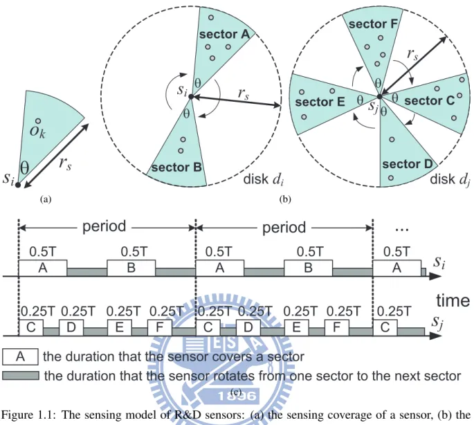
1.1 The sensing model of R&D sensors: (a) the sensing coverage of a sensor, (b) the sector regions that sensors have to rotate to cover, and (c) the rotation periods

of sensors. . . 2

4.1 An example of the modified GDC scheme. . . 12

4.2 The sector cutting operation on a disk: (a) assign indices to objects, (b) group objects into clusters, (c) merge the first cluster and the last cluster if their in-cluded angle is no larger than θ, and (d) place sectors to cover objects. . . . 13

4.3 The DOD algorithm: (a) find joint sectors of disks da and db and (b) place a sensor at location si to cover all objects in the joint sectors A, B, and E. . . . . 16

5.1 The number of deployed nodes under different number of objects in the random distribution of objects. . . 22

5.2 The number of deployed nodes under different number of objects in the cluster-based distribution of objects. . . 23

5.3 The number of sensors under different sector angles (θ) in the random distribu-tion of objects. . . 25

5.4 The number of sensors under different sector angles (θ) in the cluster-based distribution of objects. . . 26

5.5 The number of sensors under different δ values. . . . 28

5.6 The design architecture of the event-based visual surveillance system. . . 29

6.1 The object module. . . 32

6.2 The R&D sensor: (a) the infrared detector, (b) the stepper motor, and (c) the camera module (within the mobile phone). . . 33

(7)

Chapter 1 Introduction

Wireless sensor networks (WSNs) possess many charming characteristics such as ad hoc com-munication, cooperative sensing, and distributed processing. They are widely adopted in various military and civil applications [11, 31, 17]. To make a WSN well operate, sensors have to be deployed to organize a connected network that covers the whole sensing field or a set of spe-cific point-locations. Most of the WSN deployment schemes focus on omnidirectional sensors with disk-like sensing coverage [20, 27, 9]. However, in many practical WSN applications, sensors may have sector-like sensing coverage because of equipment constraints or application requirements. In addition, with the help of machinery such as stepper motors, these sensors can possess some mobility abilities such as rotation [13, 7, 8]. This type of sensor is called a

rotatable, directional (R&D) sensor.

In this paper, we consider the scenario where sensors can be precisely deployed at any location within the sensing field, and investigate how to efficiently deploy R&D sensors to monitor a given set of static objects, where each object is modeled by a point-location. The sensing coverage of each R&D sensor is modeled by a sector and the sensor can rotate to scan a whole disk, as shown in Fig. 1.1(a) and (b). The time axis is divided into fixed periods and during each period a sensor will rotate one cycle and stop to detect the objects within its sensing coverage for a total (constant) time T , as shown in Fig. 1.1(c). For example, in the beginning of

(8)

s

_i

q

r

_s

o

_k (a)

s

_i sector B

disk

d

_i sector A

r

_s

q

s

_j sector C sector D sector E

disk

d

_j sector F

r

_s

q

(b)

time

period

...

A

the duration that the sensor covers a sector

the duration that the sensor rotates from one sector to the next sector

s

_i

A

B

A

B

A

0.5T

s

_j

C

D

E

F

C

D

E

F

C

0.25T 0.25T

0.25T

(c)

Figure 1.1: The sensing model of R&D sensors: (a) the sensing coverage of a sensor, (b) the sector regions that sensors have to rotate to cover, and (c) the rotation periods of sensors. each period, sensor sifirst stops at sector A to monitor the objects in sector A for 0.5T time and

then rotates its sensing coverage to monitor the objects in sector B for another 0.5T time. Then, in the beginning of the next period, sensor si will rotate to cover sector A again. Similarly,

sensor sjwill rotate one cycle and cover the four sectors C, D, E, and F in every period, where sj will stop at each sector to monitor the corresponding objects for 0.25T time. We assume that

all R&D sensors have the same rotating speed so that each sensor will take a constant time to rotate one cycle (without stopping). In this case, each R&D sensor can have the same period length. Note that it is not necessary to synchronize the periods of sensors.

(9)

sensing coverage of one sensor for at least δT time, where 0 < δ ≤ 1. A network is said to achieve δ-time coverage if all monitored objects can be δ-time covered. Fig. 1.1(b) and (c) gives an example, where the objects in disks di and dj are 0.5-time and 0.25-time covered,

respectively, and the network can achieve 0.25-time coverage. The above temporal coverage model can be used in many WSN applications. One common example is the radar system. Another practical example is the visual surveillance system using rotatable video cameras [16]. Based on this model, we aim at the R&D sensor deployment problem, which determines how to place the minimum number of R&D sensors to cover a set of objects such that the network can achieve δ-time coverage.

The R&D sensor deployment problem is NP-hard because one of its instances is the

geo-metric disk cover (GDC) problem [30], which is a well-known NP-hard problem. Specifically,

given a set of point-locations, the GDC problem determines how to place the minimum number of disks to cover these point-locations. Consider that each R&D sensor can cover a sector with angle of θ ∈ (0, π). By making δ = θ

2π, our R&D sensor deployment problem can reduce to the

GDC problem because we can place one sensor at each disk to make all objects in that disk be

δ-time covered.

To solve the R&D sensor deployment problem, we propose two efficient heuristics. Our de-ployment idea is to first place the fewest disks to cover all objects and then deploy the minimum number of R&D sensors at some of these disks such that all objects can be δ-time covered. The first heuristic, called the maximum covering deployment (MCD) algorithm, always first places a sensor at the disk that covers the maximum number of objects. On the other hand, the second heuristic, called the disk-overlapping deployment (DOD) algorithm, takes advantage of disk overlap to reduce the number of sensors. Simulation results show that the proposed heuristics can deploy fewer R&D sensors under different distributions of objects. Specifically, the MCD

(10)

algorithm can reduce the number of sensors when objects congregate at some locations. On the other hand, when objects are arbitrarily distributed over the sensing field, the DOD algorithm can achieve a better performance.

Moreover, to demonstrate the practicability of our temporal coverage model, we develop a visual surveillance system for security applications by using R&D sensors. In our system, each R&D sensor is equipped with an infrared detector to monitor objects, a camera to provide snapshots of the environment, and a stepper motor to support the rotation capability. Initially, we adopt the proposed deployment algorithms to determine the locations to place R&D sensors. Then, each R&D sensor will rotate one cycle to scan its surrounding objects. After identifying the objects around it, the R&D sensor will follow our temporal coverage model to periodically monitor these objects (and take their snapshots accordingly). However, when one object is taken away from the sensing coverage of the R&D sensor, the sensor will be aware of the disappearance of that object when it rotates to the corresponding sector. In this case, the R&D sensor will report a warning message along with the detailed snapshots of the environment (by zooming in its camera) to the user. Compared with the traditional surveillance systems that collect a large volume of video information, our visual surveillance system is event-driven in the sense that only when objects are moved will the warning messages be sent to the users for notification. In this way, we can avoid using huge computation or even manpower to analyze a large volume of video information.

The contribution of this paper are three-folds. First, we define a new temporal coverage model for R&D sensors to monitor objects and formulate the R&D sensor deployment problem. Second, we propose two efficient deployment heuristics, the MCD and DOD algorithms, that can reduce the number of sensors under different distributions of objects. Third, we develop a prototyping system for the event-driven visual surveillance application to demonstrate the

(11)

proposed temporal coverage model.

The rest of this paper is organized as follows: Related work is surveyed in Chapter 2. Chap-ter 3 formally defines the R&D sensor deployment problem. In ChapChap-ter 4, two efficient deploy-ment heuristics are proposed. Simulation results are presented in Chapter 5. Chapter 6 gives our prototyping experience of the visual surveillance system. Finally, Chapter 7 concludes this paper.

(12)

Chapter 2 Related Work

The issue of deploying omnidirectional sensors to cover a sensing field has been extensively investigated in the literature [32]. The sensing model of these omnidirectional sensors can be either binary [27, 18] or probabilistic [12, 35]. Under the binary sensing model, the sensing coverage of a sensor is one disk and a location can be either monitored or not monitored by the sensor. On the other hand, under the probabilistic sensing model, the sensing coverage may be an arbitrary shape and a location will be monitored by the sensor with some probability function.

Many research efforts address how to use mobile, omnidirectional sensors to automatically organize a network. For example, references [34], [25], and [15] consider moving sensors to enhance the network coverage by adopting a Voronoi diagram or the attractive/repulsive forces among sensors. The work in [26] partitions the sensing field into grids, and then moves sensors from high-density grids to low-density grids to achieve a more uniform network topology. The studies in [28] and [29] address two deployment-related problems, namely the sensor placement

problem and the sensor dispatch problem. The sensor placement problem determines how to

place the minimum number of sensors to cover the whole sensing field. On the other hand, the sensor dispatch problem determines how to assign mobile sensors to move to the target locations (calculated by the placement solution) such that their moving energy can be reduced.

(13)

Several studies consider a randomly-deployed directional sensor network. The work in [6] discusses how to identify a minimal set of directions for the sensors to cover the maximum number of specific point-locations. Given a randomly-deployed sensor network, the study in [21] analyzes the probability that a point-location can be covered by directional sensors. Refer-ence [10] divides the network into subsets of sensors to alternatively cover a set of predefined point-locations, so that the energy of directional sensors can be preserved.

How to deploy static directional sensors has also been discussed in the literature. The work in [14] considers deploying a minimum number of directional sensors to organize a connected network that covers either a set of point-locations or the entire sensing field. References [23] and [22] adopt an integer linear programming manner to minimize the number of directional sensors needed to be deployed to cover a set of point-locations. However, the above studies do not consider the rotation capability of directional sensors. Using R&D sensors to localize objects is discussed in [19], but the rotation of each sensor is constrained by a limited angle. To the best of our knowledge, none of prior work addresses the R&D sensor deployment problem and the temporal coverage model. In this paper, we not only propose two efficient R&D sen-sor deployment heuristics but also implement a visual surveillance system to demonstrate the temporal coverage model by R&D sensors.

(14)

Chapter 3 Problem Definition

We are given a set of static objects bO = {o1, o2, · · · , om} to be monitored by R&D sensors,

where each object is modeled by a point-location in a two-dimensional plane. Each sensor si

has a sensing range modeled by a sector with angle of θ ∈ (0, π) and radius of rs, and possesses

an omnidirectional communication range with radius of rc, where rs and rc are the sensing

distance and the communication distance of sensors, respectively. We make no assumption on the relationship between rs and rc. We consider the binary sensing model. Thus, an object ok ∈ bO is said to be covered by a sensor si if ok locates inside the sensing coverage of si, as

shown in Fig. 1.1(a). Sensors have the rotation capability. When a sensor si rotates one cycle

(without changing its position), its sensing coverage will scan a whole disk di that is centered

at siand with radius of rs. According to the objects in disk di, we can cut diinto αi disjointed

sectors, where each sector has an angle of θ. Sensor si then rotates its sensing coverage to fit

each of these αi sectors. When the sensing coverage of sensor si completely fits a sector, we

say that sicovers that sector. Fig. 1.1(b) gives two examples. Disk diis cut into two sectors and

sensor siwill rotate to cover sectors A and B, while disk dj is cut into four sectors and sensor sj will rotate to cover sectors C, D, E, and F .

The time axis is divided into fixed-length periods. During each period, a sensor siwill rotate

(15)

corresponding sensor si will stay to cover each sector for _αT_i time and then rotate to the next

sector. Thus, the length of a period is the total time that a sensor stays to cover all sectors (that is, time T ) and the time for the sensor to rotate one cycle (marked as grey in Fig. 1.1(c)). Note that strict time synchronization of sensors is not necessary. Fig. 1.1(c) gives two examples. Because disks di and dj are cut into two and four sectors, sensors si and sj will stay to cover

each disk for 0.5T and 0.25T time, respectively.

Given a threshold δ, where 0 < δ ≤ 1, an object is said to be δ-time covered if and only if during each period, this object can be covered by one sensor for at least δT time. Fig. 1.1(c) gives two example, where objects in disks di and dj are 0.5-time and 0.25-time covered,

re-spectively. Then, given the set of objects bO and the threshold δ, our R&D sensor deployment problem determines how to place the minimum number of R&D sensors to cover all objects in

b

O such that each object can be δ-time covered. Note that in this case, each sensor can cover at

most b1

δc sectors during each period. When a disk is cut into more than b

1

δc sectors, it requires

more than one sensor to cover all of its sectors. Fig. 1.1(b) gives an example. Supposing that 0.5-time coverage is required (that is, δ = 0.5), we need to place two sensors at disk dj to make

all of its objects be 0.5-time covered.

(16)

Chapter 4 The Proposed Sensor Deployment

Algorithms

Our deployment idea is to first place the fewest disks to cover all objects and then deploy the minimum number of R&D sensors at a subset of these disks to make all objects be δ-time covered. We propose two deployment algorithms. The first MCD algorithm places sensors at those disks that cover the maximum number of objects, while the second DOD algorithm tries to reduce the number of sensors by exploiting the overlap between two disks. Then, we discuss how to add the minimum number of relay nodes to maintain the network connectivity.

4.1 The Maximum Covering Deployment (MCD) Algorithm

Given a set of objects bO to be monitored, our MCD algorithm involves the following three

phases:

• Phase 1: Calculate a set of disks bD that cover all objects in bO.

• Phase 2: Initially, all objects are unmarked. We then select the disk with the maximum

number of unmarked objects and conduct the sector cutting operation on that disk to calculate how many sectors should be placed in that disk to cover all of its unmarked objects. Then, we mark the objects in that disk. The above two operations are repeated until all objects in bO are marked. Then, we remove those disks that are not conducted

(17)

with sector cutting operation from bD.

• Phase 3: Place R&D sensors at the disks in bD to cover all objects in bO.

We then discuss the detail of each phase. In phase 1, we modify the GDC approximate solution in [30] to calculate the set of disks bD that cover all objects in bO. This modified GDC

scheme contains the three steps:

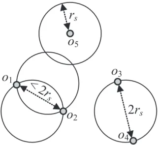
1. For any two objects oiand ojin bO, if their distance is smaller than 2rs, we place two disks

such that their circumferences intersect at oi and oj. The objects o1and o2 in Fig. 4.1 give

an example.

2. For any two objects oiand ojin bO, if their distance is equal to 2rs, we place one disk such

that its circumference passes oiand oj. The objects o3and o4in Fig. 4.1 give an example.

3. After the above two steps, there may remain some “isolated” objects whose distances to their closest objects are larger than 2rs. For each of these objects, we place one disk such

that its center is located at that object. The object o5 in Fig. 4.1 gives an example.

Because we need to check each pair of objects in bO, the maximum number of disks in bD will

be 2Cm

2 .

Then, in phase 2, we iteratively select the disk in bD that covers the maximum number of

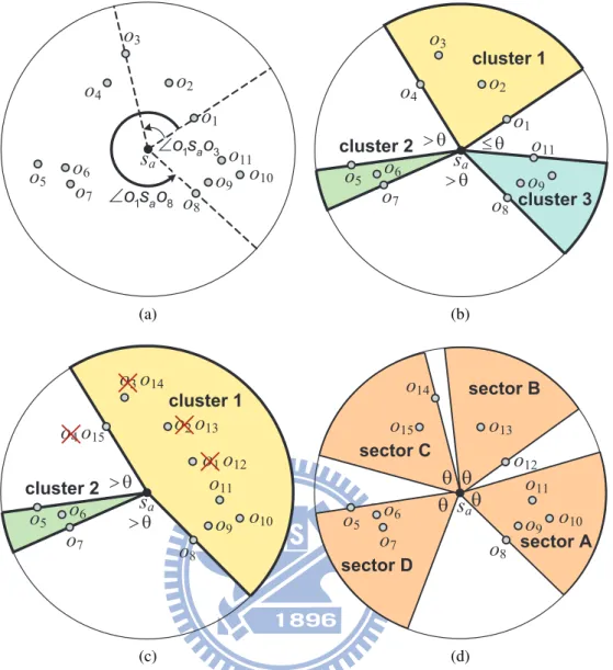
objects and conduct the sector cutting operation on that disk. The idea of this operation is to first identify where objects gather in the disk and then cluster these objects accordingly. Then, we place sectors to cover all objects in each cluster. Specifically, considering that the disk covers a set of k objects, the sector cutting operation involves the following three steps:

1. Randomly select an object, say, o1 as the initial object. We then scan the objects in

the disk counterclockwise and assign indices to these objects accordingly. In particular,

(18)

o

₁

o

₂

o

₃

o

₄

o

₅

r

_s

2r

_s

<

2r

s

Figure 4.1: An example of the modified GDC scheme.

let sa be the disk center. Object oi is assigned with a smaller index than object oj if

∠o1saoi < ∠o1saoj. Note that all angles are scanned counterclockwise. When there is

a tie, we randomly assign indices to the objects. Fig. 4.2(a) gives an example. Because ∠o1sao3 < ∠o1sao8, object o3 is assigned with a smaller index than object o8.

2. Starting from o1 and scanning objects according to their indices, we then group objects

into clusters. Object o1 is added into cluster 1. Then, for two adjacent objects oi and oi+1, 1 ≤ i ≤ k − 1, supposing that oi belongs to cluster j, object oi+1is also added into

cluster j if ∠oisaoi+1 ≤ θ. Otherwise, oi+1is added into cluster j + 1. Fig. 4.2(b) gives

an example. After grouping all objects, we then check whether or not the first cluster and the last cluster can be merged. Specifically, if ∠oksao1 ≤ θ, these two clusters can be

merged and we reindex those objects originally in cluster 1. Supposing that objects o1,

o2, · · · , and olare originally added into cluster 1, they will be assigned with new indices ok+1, ok+2, · · · , and ok+l, respectively. Fig. 4.2(c) gives an example.

3. For each cluster of objects, we place sector(s) to cover them. Specifically, starting from the uncovered object with the smallest index in the cluster, say, oi, we place a sector

(19)

sa o1 o2 o3 o5 o7 o8 o11 o4 o6 o9 o10 Ð 1 a 3 o s o Ð 1 a 8 o s o (a) sa o1 o2 o3 o5 o7 _o 8 o11 o4 cluster 1 cluster 2 cluster 3 q > q > q £ o6 o9 (b) sa o1o12 o5 o7 o8 o11 cluster 1 cluster 2 >q q > o2o13 o3o14 o4o15 o6 o9 o10 (c) sa o12 o13 o14 o7 _o 8 o11 o15 o5 q q q q o6 o9 o10 sector B sector C sector D sector A (d)

Figure 4.2: The sector cutting operation on a disk: (a) assign indices to objects, (b) group objects into clusters, (c) merge the first cluster and the last cluster if their included angle is no larger than θ, and (d) place sectors to cover objects.

whose edge passes oi such that the sector can cover the maximum number of objects in

the cluster. This operation is repeated until all objects in the cluster are covered by sectors. Fig. 4.2(d) gives an example, where sectors A, B, and C cover the objects in cluster 1 while sector D covers the objects in cluster 2.

Note that since there are m objects in bO, we will conduct the sector cutting operation on at most O(m) disks. Then, all remaining disks (without conducting the sector cutting operation) will

be removed from bD and the size of bD can shrink from O(2Cm

2 ) to O(m).

(20)

Finally, in phase 3, we place R&D sensors at the disks in bD to cover objects. In particular,

we select the disk, say, di that covers the maximum number objects when we place an R&D

sensor1_{. Then, we place a sensor at the center of disk d}

i and make the sensor rotate to cover

each of αi sectors in disk di. (When disk di has more than b1_δc sectors, these αi sectors are the

first b1

δc sectors that cover the maximum number of objects. Otherwise, αi is the total number

of sectors of disk di.) Then, we remove the objects covered by the sensor from bO. (In this

way, these αi sectors are also removed from disk di.) The above operations are repeated until

b

O becomes empty. Fig. 4.2(d) gives an example, where δ = 0.5. We first place a sensor at sa

to cover sectors A and D and remove these two sectors from the disk. Then, we place another sensor at sato cover sectors B and C. Note that a sensor will stay to cover each sector for 0.5T

time.

We then analyze the time complexity of the MCD algorithm. Running the modified GDC scheme in phase 1 requires at most O(Cm

2 ) time since we need to search any pair of objects

among m objects. In phase 2, it takes O(2Cm

2 · lg(2C2m)) = O(m2lg m) time to sort all disks

in bD (with size of 2Cm

2 ) to select disks for conducting the sector cutting operation. The sector

cutting operation totally takes O(3m) time because in each of the three steps, we have to scan at most m objects. In phase 3, we can build a maximum binary heap to maintain disks in

b

D (whose size is shrunk to O(m)), which requires at most O(m) time. Since deleting the

maximum from the heap takes O(lg m) time, it takes totally m · O(lg m) time to deploy R&D sensors at the disks in bD to cover all objects. Therefore, the time complexity of the MCD

algorithm is O(Cm

2 ) + O(m2lg m) + O(3m) + O(m) + m · O(lg m) = O(m2lg m).

1_{When a disk contains more than b}1

δc sectors, the maximum number of objects covered by an R&D sensor is

the number of objects in the first b1

δc sectors, where sectors are sorted based on to their objects in a decreasing

order. Otherwise, the maximum number of objects covered by the R&D sensor will be the total number of objects in that disk.

(21)

To summarize, the MCD algorithm prefers placing R&D sensors at those disks that cover the maximum number of objects. In this way, the MCD algorithm could well perform when objects are distributed in a non-uniform manner. In fact, the simulation results in Section ?? will show that the MCD algorithm can reduce the number of sensors when objects congregate at some locations.

4.2 The Disk-Overlapping Deployment (DOD) Algorithm

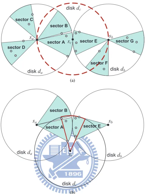
The above MCD algorithm does not take advantage of disk overlap to help reduce the number of sensors. Fig. 4.3 illustrates an example, where δ = 0.5. The MCD algorithm requires to place totally four sensors at locations saand sb to cover all objects. In fact, we can place one

sensor at location sato cover sectors C and D, one sensor at location sb to cover sectors F and G, and one sensor at location si to cover all objects in sectors A, B, and E. In this way, we

can save one sensor. Here, sectors A, B, and E are called joint sectors because they can be “jointly” covered by the third disk. Based on the above observation, our DOD algorithm tries to reduce the number of sensors by exploiting the joint sectors. The DOD algorithm is outlined as follows:

• Phase 1: Use the modified GDC scheme to find a set of disks bD. We then select a subset

of disks bDs ⊆ bD that cover all objects in bO.

• Phase 2: For any two disks in bDs, if the distance between their centers is no larger than

2rs, we find their joint sectors.

• Phase 3: For each disk in bDs, we place R&D sensor(s) to cover its sectors. When two

adjacent disks in bDs have joint sectors, we may add some R&D sensor(s) between them

to cover their joint sectors.

(22)

sb sa sc sector E sector F sector G sector A sector D sector C diskdb diskda sector B diskdc (a) sb sa sector E sector A diskdb diskda sector B si diskdi (b)

Figure 4.3: The DOD algorithm: (a) find joint sectors of disks daand db and (b) place a sensor

at location sito cover all objects in the joint sectors A, B, and E.

We then discuss the detail of each phase. In phase 1, we want to find a subset of disks bDs

from bD to cover all objects in bO such that i) the size of bDsis minimized and ii) the number of

disks that contain no more than b1

δc sectors is maximized. Objective i) is to use the fewest disks

to cover all objects. On the other hand, since we prefer the disk that can be placed with just one R&D sensor to cover all of its sectors, objective ii) is to select as more such disks as possible from bD. To achieve these two objectives, we propose a disk selection scheme as follows:

(23)

2. Select the first β > 1 disks from bD that cover the maximum number of unmarked objects

and conduct the sector cutting operation on these disks individually2_{. Then, Among these}

β disks, if there exist some disks that contain no more than b1

δc sectors, we give up

those disks that have more than b1

δc sectors (to satisfy objective ii)). However, if each of

these β disks contains more than b1

δc sectors, no disk will be given up. Then, among the

remaining disks, we select the disk, say, dithat covers the maximum number of unmarked

objects. We then mark the objects covered by disk difrom bO and add disk di into bDs.

3. Repeat step 2 until all objects in bO are marked.

Then, in phase 2, we try to find the joint sectors of any two (adjacent) disks. Specifically, two disks da and db have joint sectors if i) the distance between their centers is no larger than

2rsand ii) both disks have more than b1_δc sectors. Here, condition i) indicates that disks daand db are close enough so that we can place the third disk to overlap both of them. Condition ii) indicates that each of disks daand db requires more than one sensor to cover its sectors. In this

case, we could add sensor(s) at the third disk to jointly cover their joint sectors. Then, to find the joint sectors of disks da and db, we put a disk, say, dcsuch that its center is at the middle

of sa and sb, where sa and sb are the centers of disks da and db, respectively. A sector of disk da (respectively, db) is called a (da, db)-joint sector (respectively, a (db, da)-joint sector) if all

objects in that sector are also inside disk dc. Fig. 4.3(a) gives an example, where sectors A and B are (da, db)-joint sectors and sector E is a (db, da)-joint sector. Note that a sector may belong

to multiple joint sectors. If a sector does not belong to any joint sector, it is a non-joint sector. For example, sector F is a non-joint sector because one of its objects is not inside disk dc.

Finally, in phase 3, we place R&D sensors to cover the sectors of the disks in bDs. This phase

involves the following steps:

2_{In other words, after conducting the sector cutting operation at one disk, we do not mark those objects in that} disk.

(24)

1. For each disk diin bDswithout joint sectors, we place dαiδe sensor(s) to cover its sectors,

where αi is the total number of sectors in di. We then remove all objects in disk di from

b

O and remove disk di from bDs.

2. After step 1, bDs must remain only the disks that contain joint sectors. We then place

sensors to cover the non-joint sectors of these disks. In particular, for each disk in bDsthat contains αi > 0 non-joint sectors, we place dαiδe sensor(s) to cover its non-joint sectors.

Note that since each sensor can cover at most b1

δc sectors, there could be one sensor that

covers only, say, γ non-joint sectors, where γ < b1

δc. In this case, we make this sensor also cover the first (b1

δc − γ) joint sectors that contain the maximum number of objects.

Then, we remove all objects covered by these sensors from bO. (Those sectors and disks

contain no object are also removed accordingly.) Fig. 4.3(a) give an example. We place one sensor at location sato cover the non-joint sectors C and D in disk daand one sensor

at location sb to cover the non-joint sectors F and G in disk db. Then, only joint sectors A, B, E are left in disks daand db, as shown in Fig. 4.3(b).

3. After step 2, each disk in bDs must contain only joint sectors. Then, we select the two

disks in bDs, say, da and db, such that (da, db)-joint and (db, da)-joint sectors contain the

maximum number of objects. Let bOcbe the set of the objects covered by all (da, db)-joint and (db, da)-joint sectors. We then adopt the modified GDC scheme on bOc to calculate

a set of disks. Among these disks, we select the disk, say, di, that covers all objects

in bOc and has the fewest sectors (by conducting the sector cutting operation). We then place dαiδe sensor(s) to cover the sectors of disk di, where αiis the number of sectors of

disk di, and remove the objects in bOcfrom bO. The corresponding joint sectors are also

(25)

until bO becomes empty.

In step 3, we do not simply place sensor(s) at the middle of centers of disks daand db to cover

their joint sectors. The reason is shown in Fig. 4.3. Since the objects in the joint sectors of disks

daand db locate around location sc, it may require to place more than one sensor at location sc

to cover all objects in sectors A, B, and E. Instead, we can place just one sensor at location si

to cover all objects in these joint sectors.

We then analyze the time complexity of the DOD algorithm. In phase 1, running the modi-fied GDC scheme takes O(Cm

2 ) time and selecting the subset bDs requires O(m2lg m) + O(m)

time because we need to sort all O(m2_{) disks in b}_{D and then check at most O(m) disks from b}_D.

Because bDs contains at most O(m) disks, finding the joint sectors of any two disks in phase 2

spends O(Cm

2 ) time. Finally, in phase 3, placing sensors to cover the disks without joint sectors

in step 1 takes O(m) time. Similarly, placing sensors to cover the non-joint sectors of the disks in step 2 also requires O(m) time. Then, in step 3, conducting the modified GDC scheme on the set bOcof objects requires at most O(Cm

2 ) time. In addition, running the sector cutting operation

on the selected disk takes O(m) time. Because objects are removed when we add sensors to cover the joint sectors, the iterations in step 3 will be repeated at most O(m) times. Thus, the total time to execute step 3 is O(m · (Cm

2 + m)). Therefore, the time complexity of the DOD

al-gorithm is O(Cm

2 )+O(m2lg m)+O(m)+O(C2m)+O(m)+O(m)+O(m·(C2m+m)) = O(m3).

To summarize, the DOD algorithm exploits disk overlap to reduce the number of sensors. The simulation results in Section ?? will show that the DOD algorithm can well perform when objects are arbitrarily distributed over the sensing field.

(26)

4.3 Maintaining The Network Connectivity

Till now, our deployment algorithms focus on covering all objects. However, the network may not be connected. To solve this problem, we can place some relay nodes to maintain the network connectivity, where a relay node is the communication module of a sensor3_{. There are two}

advantages to use relay nodes to maintain the network connectivity. First, the cost to deploy the network can be reduced. Second, the deployment algorithms can allow arbitrary relationship between the sensing distance and the communication distance of sensors.

To place the minimum number of relay nodes, we modify the scheme in [14]. In partic-ular, given a set of sensors S calculated by the deployment algorithms, we first construct the minimum spanning tree on S. Then, for each tree edge whose length, say, l is larger than the communication distance rc, we place (

l

l rc

m

− 1) relay nodes along that tree edge. The distance

between two adjacent relay node is rc. The above operations are repeated until all tree edges

are checked. In this way, the network connectivity can be maintained.

(27)

Chapter 5 Performance Evaluation

We develop a simulator in C++ to verify the effectiveness of our proposed algorithms. In our simulator, the sensing field is a 400 × 400 rectangle, on which there are some objects needed to be monitored. We consider two distributions of objects. In the random distribution, objects will be uniformly, arbitrarily placed inside the sensing field. On the other hand, in the

cluster-based distribution, we arbitrarily select ten locations inside the sensing field and objects will

be placed around these locations. For comparison purpose, we develop a greedy deployment

algorithm, where a subset of objects are selected as disk centers such that these disks can cover

all objects. Then, we conduct the sector cutting operation on these disks and place R&D sensors accordingly. Each sensor has a sensing distance (rs) of 10 and a communication distance (rc)

of 20. In the DOD algorithm, we set β = 5.

5.1 Effect of The Number of Objects

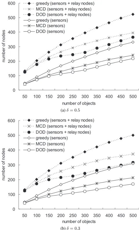
We first evaluate the effect of different numbers of objects on the number of deployed nodes by the greedy, MCD, and DOD algorithms. The number of objects is ranged from 50 to 500. The δ value is set to 0.5 and 0.3 so that a sensor can cover at most 2 and 3 sectors, respectively. The sector angle θ is set to 45◦_{. We consider the number of nodes (including sensors and}

relay nodes) needed to maintain both the object coverage and the network connectivity and the number of sensors needed to cover all objects.

(28)

0 100 200 300 400 500 600 50 100 150 200 250 300 350 400 450 500 number of objects n u m b e r o f n o d e s

greedy (sensors + relay nodes) MCD (sensors + relay nodes) DOD (sensors + relay nodes) greedy (sensors) MCD (sensors) DOD (sensors) (a) δ = 0.5 0 100 200 300 400 500 600 50 100 150 200 250 300 350 400 450 500 number of objects n u m b e r o f n o d e s

greedy (sensors + relay nodes) MCD (sensors + relay nodes) DOD (sensors + relay nodes) greedy (sensors)

MCD (sensors) DOD (sensors)

(b) δ = 0.3

Figure 5.1: The number of deployed nodes under different number of objects in the random distribution of objects.

Fig. 5.1 shows the number of deployed nodes under different number of objects in the ran-dom distribution of objects. As can be seen, when there are more objects, we need more sensors to cover them. In this case, we may also require more relay nodes to maintain the network con-nectivity. A smaller δ value can help reduce the number of sensors because each sensor can

(29)

0 50 100 150 200 250 50 100 150 200 250 300 350 400 450 500 number of objects n u m b e r o f n o d e s

greedy (sensors + relay nodes) MCD (sensors + relay nodes) DOD (sensors + relay nodes) greedy (sensors) MCD (sensors) DOD (sensors) (a) δ = 0.5 0 50 100 150 200 250 50 100 150 200 250 300 350 400 450 500 number of objects n u m b e r o f n o d e s

greedy (sensors + relay nodes) MCD (sensors + relay nodes) DOD (sensors + relay nodes) greedy (sensors)

MCD (sensors) DOD (sensors)

(b) δ = 0.3

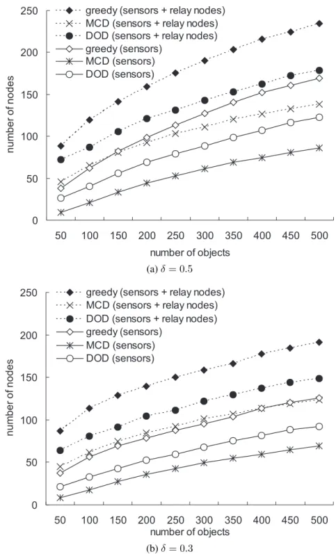
Figure 5.2: The number of deployed nodes under different number of objects in the cluster-based distribution of objects.

cover more sectors in every period. Since objects are randomly distributed, when there are fewer objects (for example, 50 objects), the number of nodes deployed by the three algorithms will be similar. On the other hand, when the number of objects grows, the difference between the number of nodes deployed by different algorithms also increases. From Fig. 5.1, we can

(30)

observe that the DOD algorithm can deploy the minimum number of nodes (that is, sensors and relay nodes) in the random distribution of objects, because it can take advantage of disk overlap to help reduce the number of sensors.

Fig. 5.2 shows the number of deployed nodes under different number of objects in the cluster-based distribution of objects. Recall that in this distribution, objects will be placed near ten locations. Thus, even though there are only 50 objects, the difference between the number of nodes deployed by different algorithms will be significant. In the cluster-based distribution of objects, the MCD algorithm can deploy the minimum number of sensors and relay nodes be-cause objects are placed near each other. In this case, deploying sensors at those disks covering the maximum number of objects can significantly reduce the number of sensors.

5.2 Effect of Sector Angle θ

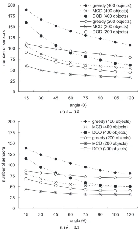
We then measure the effect of different sector angles θ on the number of deployed sensors by the greedy, MCD, and DOD algorithms. We place 200 and 400 objects and set δ values to 0.3 and 0.5. The sector angle θ is ranged from 15◦_{to 120}◦_{. We measure the number of sensors used}

to cover objects and ignore the relay nodes.

Fig. 5.3 shows the number of deployed sensors under different sector angles θ in the random distribution of objects. A larger angle θ means that a sensor can cover a wider range and thus more objects may be covered by the sensor. In this case, the number of deployed sensors can decrease when the angle θ increases. Such a trend is more significant when there are 400 objects and θ = 0.5. In this case, we need more sensors to cover objects. From Fig. 5.3, we can observe that the DOD algorithm can deploy the minimum number of sensors to cover objects under different sector angles θ in the random distribution of objects.

(31)

0 50 100 150 200 250 300 15 30 45 60 75 90 105 120 angle (è) n u m b e r o f se n so rs greedy (400 objects) MCD (400 objects) DOD (400 objects) greedy (200 objects) MCD (200 objects) DOD (200 objects) (a) δ = 0.5 0 50 100 150 200 250 300 15 30 45 60 75 90 105 120 angle (è) n u m b e r o f se n so rs greedy (400 objects) MCD (400 objects) DOD (400 objects) greedy (200 objects) MCD (200 objects) DOD (200 objects) (b) δ = 0.3

Figure 5.3: The number of sensors under different sector angles (θ) in the random distribution of objects.

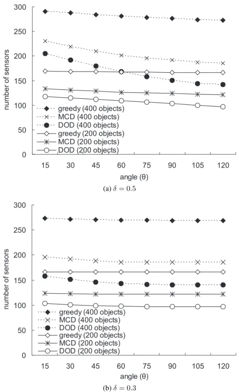
dom distribution of objects, the effect of sector angle θ is more significant in the cluster-based distribution of objects. Since objects are placed near each other, a larger angle θ can help a sensor cover more objects. In this case, the number of sensors will sharply decrease when the angle θ increases. From Fig. 5.4, we can observe that the MCD algorithm can deploy the

(32)

0 25 50 75 100 125 150 175 200 15 30 45 60 75 90 105 120 angle (è) n u m b e r o f se n so rs greedy (400 objects) MCD (400 objects) DOD (400 objects) greedy (200 objects) MCD (200 objects) DOD (200 objects) (a) δ = 0.5 0 25 50 75 100 125 150 175 200 15 30 45 60 75 90 105 120 angle (è) n u m b e r o f se n s o rs greedy (400 objects) MCD (400 objects) DOD (400 objects) greedy (200 objects) MCD (200 objects) DOD (200 objects) (b) δ = 0.3

Figure 5.4: The number of sensors under different sector angles (θ) in the cluster-based distri-bution of objects.

imum number of sensors to cover objects under different sector angles θ in the cluster-based distribution of objects.

(33)

5.3 Effect of δ Value

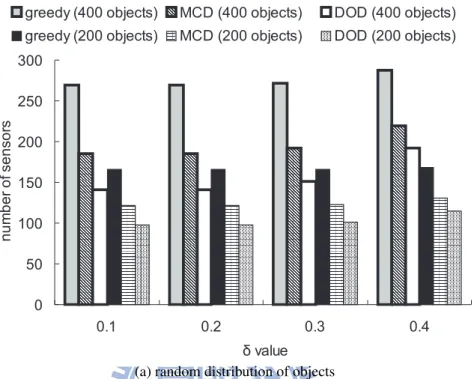
Finally, we evaluate the effect of different δ values on the number of deployed sensors by the greedy, MCD, and DOD algorithms. We place 200 and 400 objects and set the sector angle θ to 30◦_{. The δ values are set to 0.1, 0.2, 0.3, and 0.4 so that each sensor can cover at most 10, 5, 3,}

and 2 sectors in every period. Again, we calculate the number of sensors used to cover objects and ignore the relay nodes.

Fig. 5.5 shows the number of deployed sensors under different δ values. Clearly, when δ value grows, the number of sensors also increases because each sensor can cover fewer sectors in every period. Such a trend is more significant in the cluster-based distribution of objects. It can be observed that our DOD and MCD algorithms can deploy the minimum number of sensors under different δ values in the random and the cluster-based distributions of objects, respectively.

(34)

0 50 100 150 200 250 300 0.1 0.2 0.3 0.4 ä value n u m b e r o f se n so rs

greedy (400 objects) MCD (400 objects) DOD (400 objects)

(a) random distribution of objects

0 50 100 150 200 250 300 0.1 0.2 0.3 0.4 ä value n u m b e r o f s e n so rs

(b) cluster-based distribution of objects

(35)

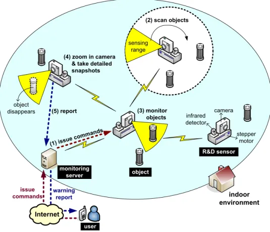
monitoring server Internet user R&D sensor issue commands warning report (4) zoom in camera & take detailed snapshots indoor environment camera infrared detector stepper motor sensing range object (1) issue comman ds (2) scan objects (3) monitor objects object disappears (5) report

Figure 5.6: The design architecture of the event-based visual surveillance system.

(36)

Chapter 6 Event-Based Visual Surveillance System

Traditional surveillance systems typically collect a large amount of videos from wall-board cameras, which require huge computation to analyze. Integrating the sensing capability of sensors can help reduce such overhead while provide more advanced, context-rich services [24]. Motivated by this observation, we develop an event-based visual surveillance system by R&D sensors.

The architecture of our event-based visual surveillance system is illustrated in Fig. 5.6. We consider an indoor environment, inside which there are several objects needed to be monitored. Each R&D sensor is equipped with an infrared detector, a camera, a wireless interface, and a stepper motor. The infrared detector has a directional sensing range and it can be used to moni-tor objects. The camera has the capability of zooming in and out to take different resolutions of snapshots from the environment. The wireless interface can communicate with the monitoring server (via multi-hop communication) to receive commands from the server or to transmit the warning messages along with snapshots to the server. The stepper motor supports the rotation capability for the R&S sensor.

We give a security scenario to illustrate how our event-based visual surveillance system works (refer to Fig. 5.6). Depending on the distribution of objects, we first determine the lo-cations to place R&D sensors by the proposed sensor deployment algorithms. In particular,

(37)

when objects congregate at some locations, the MCD algorithm can be used to deploy sensors. Otherwise, the DOD algorithm can be adopted to reduce the number of sensors. Then, the monitoring server will broadcast commands to the deployed R&D sensors, which indicate the objects needed to be monitored by the sensors. On receiving the server’s command, each R&D sensor first rotates one cycle to scan all objects around it and then monitors the specific objects (indicated by the server) following our temporal coverage model. During each rotation period, the R&D sensor will zoom out its camera to get a wider snapshot from the environment. How-ever, when one object is taken away, the R&D sensor will be aware of the disappearance of that object when it rotates to the corresponding sector. In this case, the R&D sensor will zoom in its camera to take more detailed snapshots from the environment and send the warning messages along with these snapshots to the monitoring server. In this way, the user can be notified of the movement of the object.

To make the R&D sensor correctly detect an object, each object is equipped with an object

module, as shown in Fig. 6.1. An object module is composed of an infrared receiver to obtain

the infrared signal from the R&D sensor and a Jennic board [3] for communication purpose. In particular, when the object module receives the infrared signal from an R&D sensor, it will no-tify the R&D sensor by transmitting a message through the Jennic board. We adopt the 940 nm wavelength module as the infrared receiver, which has a sensing angle of 45◦_{. The maximum}

receipt distance of the infrared receiver is 10 meters. The Jennic board is a small embedded computer that can conduct the operations of computation and wireless communication. Two Jennic boards can communicate with each other following the ZigBee standard [33].

On the other hand, an R&D sensor is composed of an infrared detector, a stepper motor, and a camera module, as shown in Fig. 6.2. The infrared detector consists of an infrared transmitter and a Jennic board. The infrared transmitter has a beam angle of 15◦ _{and we make it transmit}

(38)

infrared receiver

Jennic board

Figure 6.1: The object module.

an infrared signal every 50 milliseconds. For the stepper motor, we adopt the SANYO 103-540-1551 module [5], which can turn 1.8◦_{per step. For the camera module, we adopt the HTC Hero}

mobile phone [2] that supports the Android system [1]. When taking snapshots, the mobile phone can transmit the snapshot to the monitoring server through its wireless interface.

Fig. 6.3 shows the snapshot of our implementation, where the dashed circle is the sensing range of an R&D sensor (when it rotates one cycle). Each R&D sensor will continuously rotate to monitor the objects around it and report a warning message along with the snapshots when it finds that the object disappears. Through the above implementation, we demonstrate the feasibility of the proposed temporal coverage model.

(39)

infrared sender

Jennic board

(a)

stepper motor driver stepper

motor

(b) (c)

Figure 6.2: The R&D sensor: (a) the infrared detector, (b) the stepper motor, and (c) the camera module (within the mobile phone).

(40)

R&D sensor

stepper

motor

driver

object

module

(41)

Chapter 7 Conclusions

In this paper, we have defined a new R&D sensor deployment problem to achieve temporal cov-erage of objects and propose two efficient deployment algorithms. Our MCD algorithm deploys sensors at those disks covering the maximum number of objects. On the other hand, by exploit-ing disk overlap, our DOD algorithm tries to reduce the number of sensors by placexploit-ing them to cover the joint sectors of adjacent disks. How to place the minimum number of relay nodes to maintain the network connectivity is also addressed in the paper. Simulation results have shown that the MCD algorithm can well perform when objects congregate at some locations, while the DOD algorithm can reduce the number of sensors when objects are arbitrarily distributed over the sensing field. In addition, we have developed an event-based visual surveillance system to realize our proposed temporal coverage model. This surveillance system will provide warning messages along with detailed snapshots from the environment when objects disappear. Thus, the weakness of traditional surveillance systems can be significantly improved because only critical context information is retrieved and proactively sent to users.

(42)

Bibliography

[1] Android.

[2] HTC Hero mobile phone. [3] Jennic wireless microcontroller. [4] MOTE MICAz.

[5] SANYO stepper motor.

[6] J. Ai and A. A. Abouzeid. Coverage by directional sensors in randomly deployed wireless sensor networks. Journal of Combinatorial Optimization, 11(1):21–41, 2006.

[7] I. F. Akyildiz, T. Melodia, and K. R. Chowdhury. A survey on wireless multimedia sensor networks.

Computer Network, 51(4):921–960, 2007.

[8] S. Aoki, J. Nakazawa, and H. Tokuda. Spinning sensors: a middleware for robotic sensor nodes with spatiotemporal models. Proc. IEEE International Conference on Embedded and Real-Time

Computing Systems and Applications, pages 89–98, 2008.

[9] X. Bai, S. Kumar, D. Xuan, Z. Yun, and T. H. Lai. Deploying wireless sensors to achieve both coverage and connectivity. Proc. ACM International Symposium on Mobile Ad Hoc Networking

and Computing, pages 131–142, 2006.

[10] Y. Cai, W. Lou, M. Li, and X. Y. Li. Energy efficient target-oriented scheduling in directional sensor networks. IEEE Transactions on Computers, 58(9):1259–1274, 2009.

[11] C. Y. Chong and S. P. Kumar. Sensor networks: evolution, opportunities, and challenges.

Proceed-ings of the IEEE, (8):1247–1256, 2003.

[12] T. Clouqueur, K. K. Saluja, and P. Ramanathan. Fault tolerance in collaborative sensor networks for target detection. IEEE Transactions on Computers, 53(3):320–333, 2004.

[13] J. Djugash, S. Singh, G. Kantor, and W. Zhang. Range-only SLAM for robots operating cooper-atively with sensor networks. Proc. IEEE International Conference on Robotics and Automation, pages 2078–2084, 2006.

[14] X. Han, X. Cao, E. L. Lloyd, and C. C. Shen. Deploying directional sensor networks with guaran-teed connectivity and coverage. Proc. IEEE Conference on Sensor, Mesh and Ad Hoc

Communica-tions and Networks, pages 153–160, 2008.

[15] N. Heo and P. K. Varshney. Energy-efficient deployment of intelligent mobile sensor networks.

IEEE Transactions on Systems, Man and Cybernetics—Part A: Systems and Humans, 35(1):78–92,

2005.

[16] R. Horaud, D. Knossow, and M. Michaelis. Camera cooperation for achieving visual attention.

Machine Vision and Applications, 16(6):1–12, 2006.

[17] Y. M. Huang, M. Y. Hsieh, H. C. Chao, S. H. Hung, and J. H. Park. Pervasive, secure access to a hierarchical sensor-based healthcare monitoring architecture in wireless heterogeneous networks.

IEEE Journal on Selected Areas in Communications, 27(4):400–411, 2009.

[18] K. Kar and S. Banerjee. Node placement for connected coverage in sensor networks. Proc.

(43)

[19] J. Y. Lee. Exploiting constrained rotation for localization of directional sensor networks. Proc.

IEEE International Wireless Communications and Mobile Computing Conference, pages 767–772,

2008.

[20] F. Y. S. Lin and P. L. Chiu. A near-optimal sensor placement algorithm to achieve complete cover-age/discrimination in sensor networks. IEEE Communication Letters, 9(1):43–45, 2005.

[21] H. Ma and Y. Liu. Some problems of directional sensor networks. International Journal of Sensor

Networks, 2(1/2):44–52, 2007.

[22] Y. Osais, M. St-Hilaire, and F. R. Yu. On sensor placement for directional wireless sensor networks.

Proc. IEEE International Conference on Communications, 2009.

[23] Y. Osais, M. St-Hilaire, and F. R. Yu. The minimum cost sensor placement problem for directional wireless sensor networks. Proc. IEEE Vehicular Technology Conference, 2008.

[24] Y. C. Tseng, Y. C. Wang, K. Cheng, and Y. Y. Hsieh. iMouse: an integrated mobile surveillance and wireless sensor system. Computer, 40(6):60–66, 2007.

[25] G. Wang, G. Cao, and T. L. Porta. Movement-assisted sensor deployment. Proc. IEEE INFOCOM, pages 2469–2479, 2004.

[26] G. Wang, G. Cao, T. L. Porta, and W. Zhang. Sensor relocation in mobile sensor networks. Proc.

IEEE INFOCOM, pages 2302–2312, 2005.

[27] Y. C. Wang, C. C. Hu, and Y. C. Tseng. Efficient deployment algorithms for ensuring coverage and connectivity of wireless sensor networks. Proc. IEEE Wireless Internet Conference, pages 114–121, 2005.

[28] Y. C. Wang, C. C. Hu, and Y. C. Tseng. Efficient placement and dispatch of sensors in a wireless sensor network. IEEE Transactions on Mobile Computing, 7(2):262–274, 2008.

[29] Y. C. Wang and Y. C. Tseng. Distributed deployment schemes for mobile wireless sensor networks to ensure multilevel coverage. IEEE Transactions on Parallel and Distributed Systems, 19(9):1280– 1294, 2008.

[30] B. Xiao, Q. Zhuge, Y. He, Z. Shao, and E. H. M. Sha. Algorithms for disk covering problems with the most points. Proc. IASTED International Conference on Parallel and Distributed Computing

and Systems, pages 541–546, 2003.

[31] L. W. Yeh, Y. C. Wang, and Y. C. Tseng. iPower: an energy conservation system for intelligent buildings by wireless sensor networks. International Journal of Sensor Networks, 5(1):1–10, 2009. [32] M. Younis and K. Akkaya. Strategies and techniques for node placement in wireless sensor

net-works: a survey. Ad Hoc Networks, 6(4):621–655, 2008.

[33] ZigBee specification version 2006, ZigBee document 064112, 2006.

[34] Y. Zou and K. Chakrabarty. Sensor deployment and target localization based on virtual forces.

Proc. IEEE INFOCOM, pages 1293–1303, 2003.

[35] Y. Zou and K. Chakrabarty. A distributed coverage- and connectivity-centric technique for selecting active nodes in wireless sensor networks. IEEE Transactions on Computers, 54(8):978–991, 2005.