頻率選擇性衰減通道中對於外層渦輪碼正交頻分複用系統之內層迴旋碼設計

國

立

交

通

大

學

電信工程研究所

碩

士

論

文

頻率選擇性衰減通道中對於外層渦輪碼正交頻分複用系統之

內層迴旋碼設計

Design of Non-coherent Inner Convolutional Codes

for Turbo-Coded OFDM System Over Frequency-Selective Fading Channels

研 究 生：呂志文

指導教授：陳伯寧 教授

頻率選擇性衰減通道中對於外層渦輪碼正交頻分複用系統之內層迴旋

碼設計

Design of Non-coherent Inner Convolutional Codes

for Turbo-Coded OFDM System Over Frequency-Selective Fading Channels

研 究 生：呂志文 Student：Chih-Wen Lu

指導教授：陳伯寧 Advisor：Po-Ning Chen

國 立 交 通 大 學

電信工程研究所

碩 士 論 文

Submitted to Institute of Communication Engineering College of Electrical and Computer Engineering

National Chiao Tung University in partial Fulfillment of the Requirements

for the Degree of Master

in

Communication Engineering

July 2013

tt

頻

頻

頻

率

率

率選

選

選擇

擇

_擇性

_性

_性衰

衰

衰減

減通

減

通

通道

道

道中

中

中對

對

對於

於

於外

外

外層

層

層渦

渦

渦輪

輪

輪碼

碼

_碼正

_正

_正交

交

交頻

頻

頻分

分

分

複

複

複用

用

用系

系

系統

統

統之

之

之

內

內

內

層

層

層迴

迴

迴旋

旋

旋 碼

碼

碼設

設

設計

計

計

Design of Non-coherent Inner Convolutional Codes for

Turbo-Coded OFDM System Over Frequency-Selective

Fading Channels

Student: Chih-Wen Lu kkk Advisor: Po-Ning Chen

Institute of Communications Engineering National Chiao Tung University

Abstract

In frequency-selective fading channels with unknown channel coefficients, channel esti-mation and equalization become infeasible. In this thesis, based on the cumulative distance functions of codes, we propose a simple method to select an inner convolutional code to co-work with an outer turbo code, which acts implicitly as a channel estimator and equal-izer. Since the codeword length of the selected convolutional code is short, an exhaustive decoder based on the GLRT criterion can be implemented at the receiver end. Simulation results show that the concatenated coding system that use the convolutional codes of rate 1/2 performs well but may have rooms for improvement when the inner code rate increase to 2/3. In comparison with the tradition system that employs a least square (LS) estimator for the outer turbo code, our proposal can result in better performances and hence can be a good candidate design in a blind frequency-selective fading environment.

Acknowledgements

To begin with, I would like to sincerely appreciate my advisor, Prof. Po-Ning Chen, for his patient advising and guidance. I also would like to thank the members in the NTL-lab, who gave me support when I got problems. At last, I would like to show my deepest gratitude to my parents for their nurture and love.

Contents

2.1 A non-coherent OFDM system . . . 3 2.2 Least Square Estimator for Fading Channels . . . 7 2.3 GLRT Detection . . . 8

3.1 Finding a Good Noncoherent Convolutional Code for Turbo-Coded OFDM

System: The Approach . . . 10

3.2 Concatenated Coding System Under an Unknown Fading Channel . . . 12

3.2.1 A Review of Turbo Coding . . . 13

3.2.2 Non-Coherent Convolutional Code and Exhausted Decoder . . . 14

4 Simulation Results 16 4.1 System Settings . . . 16

4.2 Remarks . . . 29

5 Conclusion and Future Work 38

List of Figures

3.1 Concatenated encoding (above) and decoding (below) systems under an un-known frequency-selective fading channel. The non-coherent transmitter (resp., receiver) includes a turbo encoder (resp., decoder), a convolutional encoder (resp., decoder), and an OFDM modulater (resp., demodulator). The GLRT detecter is also employed at the receiver. . . 12 3.2 Architecture of the turbo encoder . . . 14 3.3 The (3,2) non-coherent convolutional code which generating polynomial [5 6

0 ; 0 7 5]. . . 15

4.1 Performances of non-coherent convolutional codes under blind fading chan-nels. Here, the codeword length N = 10 and the channel memory order is ν = 2. The code rate is 1/2. . . . 19 4.2 Cumulative distance function (CDF) of the convolutional codes under test.

Here, we provide two plots that have different x-axis ranges to facilitate our interpretation of the results. The code rate is 1/2. . . . 20 4.3 Performances of non-coherent convolutional codes under blind fading

chan-nels. Here, the codeword length N = 10 and the channel memory order is ν = 2. The code rate is 1/2. . . . 21

4.4 Cumulative distance function (CDF) of the convolutional codes under test. Here, we provide two plots that have different x-axis ranges to facilitate our interpretation of the results. The code rate is 1/2. . . . 22 4.5 Performances of the concatenated coding system. The turbo code used is the

(37, 21) code proposed by Berrou and Glavieux in [7]. The codeword lengths of the type 1, 2 and 3 convolutional codes are ten, eight and six, respectively. The inner convolutional code rate is 2/3 and the outer turbo code rate is 1/3. 23 4.6 Performances of the concatenated coding system. The turbo code used is the

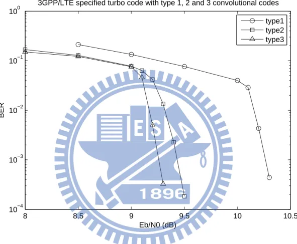
one specified in 3GPP/LTE. The codeword lengths of the type 1, 2 and 3 con-volutional codes are ten, eight and six, respectively. The inner concon-volutional code rate is 2/3 and the outer turbo code rate is 1/3. . . . 24 4.7 Performances of the concatenated coding system. The turbo code used is the

one specified in [11]. The codeword lengths of the type 1, 2 and 3 convolutional codes are ten, eight and six, respectively. The inner convolutional code rate is 2/3 and the outer turbo code rate is 1/3. . . . 25 4.8 Performances of a conventional system that employs the (37, 21) turbo code

[7] with a least square (LS) channel estimator instead of our non-coherent convolutional code. Here, type 1, type 2 and type 3 similarly denote the sizes of the LS estimator, i.e., 10, 8 and 6. The inner LS channel estimator rate is 2/3 and the outer turbo code rate is 1/3. The curves in Figure 4.5 are also illustrated for comparison. . . 26

4.9 Performances of a conventional system that employs the 3GPP/LTE specified turbo code [12] with a least square (LS) channel estimator instead of our non-coherent convolutional code. Here, type 1, type 2 and type 3 similarly denote the sizes of the LS estimator, i.e., 10, 8 and 6. The inner LS channel estimator rate is 2/3 and the outer turbo code rate is 1/3. The curves in Figure 4.6 are also illustrated for comparison. . . 27 4.10 Performances of a conventional system that employs the turbo code from

[11] with a least square (LS) channel estimator instead of our non-coherent convolutional code. Here, type 1, type 2 and type 3 similarly denote the sizes of the LS estimator, i.e., 10, 8 and 6. The inner LS channel estimator rate is 2/3 and the outer turbo code rate is 1/3. The curves in Figure 4.7 are also illustrated for comparison. . . 28 4.11 Performances of the concatenated system that employs the (37, 21) turbo code

[7] concatenated with the non-coherent convolutional codes of type 0, 1, 2, 3. Here, the codeword lengths at type 0, 1, 2, 3 codes are respectively 12, 10, 8 and 6. The inner convolutional code rate is 2/3 and the outer turbo code rate is 1/3 . . . . 32 4.12 Performances of the concatenated system that employs the 3GPP/LTE

spec-ified turbo code [12] concatenated with the non-coherent convolutional codes of type 0, 1, 2, 3. Here, the codeword lengths at type 0, 1, 2, 3 codes are respectively 12, 10, 8 and 6. The inner convolutional code rate is 2/3 and the outer turbo code rate is 1/3 . . . . 33

4.13 Performances of the concatenated system that employs the turbo code from [11] concatenated with the non-coherent convolutional codes of type 0, 1, 2, 3. Here, the codeword lengths at type 0, 1, 2, 3 codes are respectively 12, 10, 8 and 6. The inner convolutional code rate is 2/3 and the outer turbo code rate is 1/3 . . . . 34 4.14 Performances of the concatenated system that employs the (37, 21) turbo code

[7] concatenated with the optimal non-coherent convolutional codes of type 2 and 3. The inner convolutional code rate is 1/2 and the outer turbo code rate is 1/3 . . . 35 4.15 Performances of the concatenated system that employs the 3GPP/LTE

speci-fied turbo code [12] concatenated with the optimal non-coherent convolutional codes of type 2 and 3. The inner convolutional code rate is 1/2 and the outer turbo code rate is 1/3 . . . 36 4.16 Performances of the concatenated system that employs the turbo code from

[11] concatenated with the optimal non-coherent convolutional codes of type 2 and 3. The inner convolutional code rate is 1/2 and the outer turbo code rate is 1/3 . . . 37

Chapter 1

Introduction

1.1

Overview

In this thesis, we research on the transceiving of orthogonal frequency-division multiplexing (OFDM) modulated signals [1] over the unknown frequency-selective fading channels.

In the past decades, separate channel estimation and channel equalization have been the major demodulation technologies for communication systems over fading channels [2, 3]. However, such a system structure may not be well suited for a highly mobile environment, which somehow motivates the use of noncoherent detection for communications among mov-ing objects.

By [4], non-coherent detection jointly estimates the channel and data, and are often regarded as a generalized likelihood ratio test (GLRT). It does not require a separate train-ing sequence for the estimation and equalization of channel fadtrain-ing effects. Under a blind environment, researches have shown that the GLRT demodulator can provide the best per-formance [5, 6].

At this background, we propose an error correcting coding scheme that concatenates the turbo code [7] (as an outer code) and the convolutional code (as an inner code) in sequence to alleviate the need of channel estimation and equalization. The convolutional

code is specifically designed for blind detection over fading channels. By analyzing the Euclidean distance among codewords [5] at the output of convolutional encoders, we provide a general method to determine which convolutional coding structure can yield a seemingly best performance in the sense of bit error rate (BER) under a blind environment. The proposed concatenated system is then compared with the conventional structure, where a turbo code is supported by a least square (LS) channel estimator [8] in stead of our convolutional code, provided that both systems have the same system transmission rate including the training sequence used for least square estimation.

The remaining of the thesis is organized as follows. Chapter 2 surveys some background technologies for this thesis, which includes non-coherent OFDM system, least square estima-tion and GLRT demodulaestima-tion. Chapter 3 describes the proposed method on determinaestima-tion of the seemingly best convolutional code for a blind environment, as well as the entire sys-tem we construct for unknown frequency-selective fading channels. Chapter 4 presents the simulation results, while Chapter 5 concludes the thesis.

1.2

Notations

Symbol Meaning

x a vector in time domain

X a vector in frequency domain

Q a matrix

∥X∥ the norm of a vector X

⃗

S a combination of vectors

XT _{transpose of a vector X}

X† Hermitian transpose of a vector X

Chapter 2

Preliminaries

In this chapter, the background knowledge on orthogonal frequency-division multiplexing (OFDM), the least square channel estimator, and generalized likelihood ratio test (GLRT) is introduced. Specifically, Section 2.1 presents the non-coherent OFDM system over fading channels, Section 2.2 provides the least square estimation for fading channels by following [9], and Section 2.3 gives the basic conception of GLRT-based signal detection.

2.1

A non-coherent OFDM system

In this thesis, we consider an OFDM system of N subchannels, for which binary phase-shift keying (BPSK) signals are non-coherently transmitted over a frequency-selective fading channel with fading coefficients h = [hν · · · h1 h0

]T

unknown to both the transmitter and receiver.

Denote the information transmitted at time j as

Sj =      S1,j S2,j .. . SN,j      N×1 ,

the information is transformed to its time-domain counterpart as sj =Q†Sj =      s1,j s2,j .. . sN,j      N×1

where the superscript ”†” indicates the matrix Hermitian transpose operation and the DFT matrix is given by Q = √1 N        e−i2πN(N−1)(N−1) e−i 2π N(N−2)(N−1) · · · e−i 2π N(N−1) 1 e−i2πN(N−1)(N−2) e−i 2π N(N−2)(N−2) · · · e−i 2π N(N−2) 1 .. . ... . .. ... ... e−i2πN(N−1) e−i 2π N(N−2) · · · e−i 2π N 1 1 1 · · · 1 1        N×N (2.1)

Afterwards, a cyclic prefix [10] of length ν is added to the time-domain information sj before its transmission over the fading channel, resulting a transmission signal of length L = N + ν:

pj =      p1,j p2,j .. . pL,j     =              s1,j s2,j .. . sN,j s1,j s2,j .. . sν,j              L×1

When transmitting pj non-coherently over a fading channel, we should consider the impact of both the unknown channel coefficients and the background noise. Thus, the channel model is given by:

yj =      y1,j y2,j .. . yL,j     =            h0 h1 · · · hν 0 · · · 0 0 h0 · · · hν−1 hν · · · 0 .. . ... . .. ... ... . .. ... 0 0 · · · h0 h1 · · · hν 0 0 · · · 0 h0 · · · hν−1 .. . ... . .. ... ... . .. ... 0 0 · · · 0 0 · · · h0                 p1,j p2,j .. . pL,j     +      v1,j v2,j .. . vL,j      (2.2)

where vj =      v1,j v2,j .. . vL,j     

represents a zero-mean additive Gaussian noise vector and v1,j, v2,j· · · , vL,j are independent and identically distributed (i.i.d.) with covariance matrix σ2I

L. In this thesis,IL denotes an

L× L identity matrix.

After the reception of yj, the cyclic prefix will be removed first, yielding a received vector of size N as: xj =      x1,j x2,j .. . xN,j     =      y1,j y2,j .. . yN,j     . By (2.2), we know that xj =            h0 h1 · · · hν−1 hν 0 · · · 0 0 h0 · · · hν−2 hν−1 hν · · · 0 .. . ... . .. ... ... ... . .. ... 0 0 · · · 0 h0 h1 · · · hν hν 0 · · · 0 0 h0 · · · hν−1 .. . ... . .. ... ... ... . .. ... h1 h2 · · · hν 0 0 · · · h0                 s1,j s2,j .. . sN,j     +      v1,j v2,j .. . vN,j      = Hsj+ wj where wj = [ w1,j w2,j· · · wN,j ]T = [v1,j v2,j· · · vN,j ]T

. Since H is a circulant matrix, we can decompose it as:

H = Q†_{ΛQ = Q}†      λN−1 0 · · · 0 0 λN−2 · · · 0 .. . ... . .. ... 0 0 · · · λ0     Q (2.3)

where the definition of Q can be found in (2.1), and Λ is a diagonal matrix with diagonals

λ =[λN−1 λN−2 · · · λ0

]T

as indicated above. We can thus rewrite (2.3) as:

xj =Q†ΛQsj+ wj. (2.5)

By QQ†=I, we can transform (2.5) into its frequency-domain counterpart as:

Xj =Qxj =QQ†ΛQsj+Qwj = ΛSj+ Wj

where Sj = Qsj and Wj = Qwj are the discrete Fourier transforms (DFTs) of signals sj and wj, respectively. For derivation convenience, we rewrite the above system as:

Xj =Sjλ + Wj

where λ is defined in (2.4) and Sj is the diagonal matrix corresponding to Sj, which is given by: Sj =      S1,j 0 · · · 0 0 S2,j · · · 0 .. . ... . .. ... 0 0 · · · SN,j      N×N

We next introduce non-coherent OFDM detection. Under the assumption that both the transmitter and receiver know nothing about the channel coefficients, it can be derived that at least two OFDM symbols are needed to secure the detection error being better than that of a random guess. Thus, we assume that T ≥ 2Ts, where T is the period, during which fading coefficients h remain constant, and Ts is the symbol duration of an OFDM symbol. For simplicity, we suppose two OFDM symbols are used for non-coherent detection at the receiver end, and its extension to more OFDM symbols can be similarly done. Let the two OFDM symbols be:

X1 =S1λ + W1 (2.6)

and

We then combine for convenience (2.6) and (2.7) into: ⃗ X = ⃗Sλ + ⃗W (2.8) where ⃗ X = [ X1 X2 ] , S =⃗ [ S1 S2 ] and W =⃗ [ W1 W2 ] . Again, we can multiplex k OFDM symbols to make ⃗S =[S1 S2· · · Sk

]T

if T > kTs. However, the system complexity will significantly grow as k getting large. In addition, the requirement of T ≥ kTs will restrict the applicability of our design to a less mobile environment for a moderately large k. For these reasons, we will focus only on the case of k = 2 in this thesis.

2.2

Least Square Estimator for Fading Channels

Consider the system model introduced in Section 2.1. Upon the reception of ⃗X, the receiver

intends to estimate λ such that ∥ ⃗X − ⃗Sλ∥2 _{is minimized when ⃗S is assumed known. This}

is therefore named the least square estimator (LSE). Denoting ⃗Z = ⃗Sλ, we derive

J (λ) = ∥ ⃗X− ⃗Z∥2

= ( ⃗X − ⃗Sλ)T_{( ⃗X}− ⃗Sλ)

= X⃗T_{X⃗ − ⃗X}T_{Sλ⃗ − λ}T_S⃗T_{X + λ⃗} T_S⃗T_Sλ.⃗

Note that ⃗XT_{X is a constant scalar and hence we obtain the LSE of λ as:}⃗

ˆ

λ = ( ⃗STS)⃗ −1S⃗TX.⃗ (2.9) With the availability of ˆλ, the estimated channel matrix ˆH can be computed through (2.3).

Together with the turbo coding, the LSE provides a conventional system design to combat the channel fading. This conventional system will be used as a benchmark to be compared with our proposed non-coherent scheme in this thesis.

2.3

GLRT Detection

As mentioned at the beginning of Section 2.1, λ that is used to determine H through (2.3) is unknown to the system. As no training sequence is presumed, its least square estimation cannot be practiced. However, by noting that what we really desire is the estimate of the transmitted signal ⃗S, a so-called general LRT (GLRT) detection has been proposed.

The GLRT criterion can be devised as follows. ˆ ⃗ S = arg min ⃗ S∈S ( min λ∈CN∥ ⃗X− ⃗Sλ∥ 2 ) = arg min ⃗ S∈S ∥ ⃗ X− ⃗S ˆλ∥2 (2.10) = arg min ⃗ S∈S ∥ ⃗ X− P_S⃗X⃗∥2 (2.11)

where C is the set of complex numbers, S is the set of all possible transmission signal ⃗S, ˆλ in (2.10) is given by (2.9), and P_S⃗ = S( ⃗⃗ S†S)⃗ −1S⃗† = S⃗      1 |S1,1|2+|S1,2|2 0 · · · 0 0 _|S 1 2,1|2+|S2,2|2 · · · 0 .. . ... . .. ... 0 0 · · · 1 |SN,1|2+|SN,2|2     S⃗† =                   |S1,1|2 |S1,1|2+|S1,2|2 0 · · · 0 S1,1S1,2∗ |S1,1|2+|S1,2|2 0 · · · 0 0 |S2,1|2 |S2,1|2+|S2,2|2 · · · 0 0 S2,1S2,2∗ |S2,1|2+|S2,2|2 · · · 0 .. . ... . .. ... ... ... . .. ... 0 0 · · · |SN,1|2 |SN,1|2+|SN,2|2 0 0 · · · SN,1SN,2∗ |SN,1|2+|SN,2|2 S∗1,1S1,2 |S1,1|2+|S1,2|2 0 · · · 0 |S1,2|2 |S1,1|2+|S1,2|2 0 · · · 0 0 S2,1∗ S2,2 |S2,1|2+|S2,2|2 · · · 0 0 |S2,2|2 |S2,1|2+|S2,2|2 · · · 0 .. . ... . .. ... ... ... . .. ... 0 0 · · · S∗N,1SN,2 |SN,1|2+|SN,2|2 0 0 · · · |SN,2|2 |SN,1|2+∥SN,2∥2                   . (2.12)

Taking (2.12) into (2.11) yields: ˆ ⃗ S = arg min ⃗ S∈S ∥ ⃗X − P_S⃗X⃗∥2 = arg max ⃗ S∈S ⃗ X†P_S⃗X⃗ = arg max ⃗ S∈S N ∑ i=1

|Xi,1|2|Si,1|2+|Xi,2|2|Si,2|2+ Xi,1Si,1∗ Xi,2∗ Si,2+ Xi,1∗ Si,1Xi,2Si,2∗

|Si,1|2+|Si,2|2 = arg max ⃗ S∈S N ∑ i=1

|Si,1Xi,1∗ + Si,2Xi,2∗ | 2

The resulting formula forS implies that the receiver cannot distinguish between (S⃗ˆ i,1, Si,2) = (1,−1) and (Si,1, Si,2) = (−1, 1), and also (Si,1, Si,2) = (1, 1) and (Si,1, Si,2) = (−1, −1). Consequently, we shall fix one of Si,1 and Si,2 to ensure the detectability of information at the receiver. We end this subsection by providing an example of detectable information assignment: ⃗ S = [ S1 S2 ] =                  S1,1 0 0 · · · 0 0 −1 0 · · · 0 0 0 −1 · · · 0 .. . ... ... . .. ... 0 0 0 · · · SN,1 −1 0 0 · · · 0 0 S2,2 0 · · · 0 0 0 S3,2 · · · 0 .. . ... ... . .. ... 0 0 0 · · · −1                  .

Chapter 3

Design of Inner Convolutional Code

for Turbo-Coded OFDM System

In this chapter, we will introduce how we determine a convolutional code that can provide a seemingly best performance, when it is co-worked with an outer turbo code, under channels with unknown fading coefficients. In addition, the entire inner and outer concatenated coding system will be defined.

3.1

Finding a Good Noncoherent Convolutional Code

for Turbo-Coded OFDM System: The Approach

In order to construct a good convolutional coding structure without resorting to simulations, we adopt the “non-coherent” Euclidean distances (defined later in (3.1)) among codewords as our design criterion. This quantity may be computable directly and is seemingly related to the true error rate of the resulting code.

Consider the system that transmits a convolutional codeword b = [b1 b2 · · · bN ]

of length N over a frequency-selective fading channel as follows:

where the codeword matrix is given by: B =              b1 0 · · · 0 b2 b1 . .. 0 .. . ... . .. ... bN bN−1 . .. 0 0 bN . .. b1 .. . ... . .. ... 0 0 · · · bN              L×P

with L = N + ν, h is the channel coefficient vector of length P = ν + 1, and v is a zero-mean additive white Gaussian noise vector. Note that in the above formula, ν is the memory order of the channel. Then, it can be derived that the “non-coherent” Euclidean distance between codewords i and j can be used to optimally detect the optimal codeword, which is defined as:

di,j =∥vec(PBi)− vec(PBj)∥

2 _(3.1)

where

PB =B(BTB)−1BT.

In order to analyze the cumulative distribution function (CDF) of the “noncohrent” Eu-clidean distances of a convolutional codeword, we quantify di,j into 1000 levels and compute the CDF functions for two convolutional codes to be compared. Denote by CM and CN the CDF functions of two convolutional codes with structure M and N , respectively. We then do the following computation in which we only take half of the level function values for this comparison: a = 500 ∑ level=1 index(level) (3.2) where index(level) =    1, if CM(level) < CN(level) −1, if CM(level) > CN(level) 0, otherwise. (3.3)

From our observations, we note that if a > 0, then structure M mostly will yield a better performance than structure N . Hence, we propose to compare all the convolutional code design through this way, and determine the best one that with high possibility can yield a good (near optimal) error performance. We will later confirm our proposal via simulations. Note that since the designed convolutional code will be co-worked with a turbo code, the convolutional code rate that we target in this research is 2/3 (instead of the usual 1/2). This convolutional code rate, when combined with an 1/3 turbo code, will give a system code rate of (2/3)(1/3) = (2/9). Details will be given in the next section.

3.2

Concatenated Coding System Under an Unknown

Fading Channel

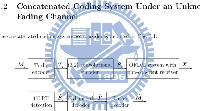
The concatenated coding system we consider is depicted in Fig. 3.1.

- Turbo - -

-encoder

(3,2) convolutional encoder

OFDM system with non-coherent receiver Mj Tj Sj Xj - -Exhausted decoder Turbo decoder ˆ Tj Mˆj GLRT detection -ˆ Sj

Figure 3.1: Concatenated encoding (above) and decoding (below) systems under an unknown frequency-selective fading channel. The non-coherent transmitter (resp., receiver) includes a turbo encoder (resp., decoder), a convolutional encoder (resp., decoder), and an OFDM modulater (resp., demodulator). The GLRT detecter is also employed at the receiver.

The idea behind our concatenated system, where we use the turbo code as an outer code and our non-coherent convolutional code as an inner code, is that the traditional turbo code design is based on the assumption that the system can perfectly recover the fading effect and

suffers only the additive white Gaussian noise. However, this may not be entirely valid in practical application. So instead of targeting a perfect channel estimator and equalizer, we use a non-coherent convolutional code, and are exempt from the need of designing channel estimator and equalizer.

Considering the code rate loss, we employ (non-coherent) convolutional codes of rate 2/3. Since our codeword length is small, an exhausted decoder can be implemented at the receiver. This is a replacement of the channel estimation and equalization on the channel fading effect with error protection enhancement. By this way, we can use the turbo outer code under a “blind” fading environment.

3.2.1

A Review of Turbo Coding

As shown in Fig. 3.2, a turbo encoder is structured with two recursive systematic convo-lutional (RSC) codes and one interleaver. In this thesis, three turbo codes with different RSC component codes and interleavers will be tested. They are respectively the (37,21) turbo code proposed by Berrou and Glavieux, one of the 3GPP/LTE specified turbo codes, and the turbo code with generator matrix [1 (1 + D + D2_{+ D}4_{)/(1 + D}3 _{+ D}4₎] _{plus a}

uniform interleaver as introduced in Shu Lin’s book. To test how effective our internal non-coherent convolutional code is, we choose a practically short codeword length for the turbo code instead a usually long one. Thus, the codeword lengths for the three turbo codes are respectively 12288, 12288, and 3000, with information lengths respectively to be 4096, 4096 and 1000.

The decoding mechanism for turbo codes is the the maximum a posteriori probability (MAP) algorithm, which after a few iterations declares whether each information bit is 1 or

-? -interleaver RSC code RSC code Xk Xk Zk X_k′ Z_k′

Figure 3.2: Architecture of the turbo encoder 0 according to the log-likelihood ratio (LLR):

Λ(i) = logPr(ci = 1| r) Pr(ci = 0| r) = log ∑ (Siw−1,Swi¯)∈B (1) i Pr(S_wi−1, S_wi_¯, r) ∑ (Siw−1,Swi¯)∈B (0) i Pr(S_wi−1, S_wi_¯, r) ,

where r is the received vector, andB_i(k) denotes the set of all transitions from nodes at level i−1 to nodes at level i corresponding to input ci = k ∈ {0, 1}. Again, we remind the readers that Si

w means the trellis state at level i. Apparently, the decision rule shall be ˆmi = 1 if Λ(i) > 0, and ˆmi = 0, otherwise.

3.2.2

Non-Coherent Convolutional Code and Exhausted Decoder

The non-coherent convolutional codes that we designed and tested in this thesis have three different codeword lengths: six, eight, and ten. For convenience, we will refer to them as type 3, type 2 and type 1 in the figures. Using the selection approach we propose, we found that the best type 1, type 2 and type 3 (3, 2) non-coherent convolutional codes are [5 6 0 ; 0 7 5], [5 6 0 ; 0 7 5] and [7 6 0 ; 0 7 5] (in octal) under unknown fading channels. As an example, the structure of the type 1 non-coherent convolution code is depicted in Fig. 3.3.

h + h + h + - -- -1 i z ? 1 6i z 9 -z−1 z−1 z−1 z−1

Figure 3.3: The (3,2) non-coherent convolutional code which generating polynomial [5 6 0 ; 0 7 5].

decoder to secure the optimal performance for the adopted code. The simulation results of the designed codes of all three types will be provided and remarked in the next chapter.

Chapter 4

Simulation Results

In this chapter, we will examine how well our proposed method can locate a non-coherent con-volutional code with acceptably good performance. Simulations on the found non-coherent convolutional codes concatenated with turbo codes will follow. For clarity, basic simulation results are provided in Section 4.1, and discussions on them as well as additional simulations to verify our interpretation will be placed in Section 4.2.

4.1

System Settings

In finding the optimal convolutional coding structure that gives the minimum decoding error, we first examine the relation between the convolutional code structures and corresponding minimum pair-wise non-coherent distances defined in (2.11).

In Figure 4.1, the legend mark “5-1;0.94” means that the convolutional code structure is defined via generator matrix

[

1 + D2 _D2]_{and its resulting minimum pairwise non-coherent}

distance is 0.94. Similarly, the codes marked 2”, 3”, 4”, 5”, 6” and “5-7” are defined via the generator matrices

[ 1 + D2 D ] , [ 1 + D2 D + D2 ] , [ 1 + D2 1 ] , [ 1 + D2 1 + D2 ] , [ 1 + D2 1 + D ] and [ 1 + D2 1 + D + D2 ]

, respectively. The simu-lation result shows that the minimum pairwise non-coherent distance may not be a good

decisive factor for performance. In particular, the one with the largest minimum pairwise non-coherent distance, i.e., “5-5”, turns out to have the worst performance. Numbers of codeword pairs that result in the respective non-coherent distances should be taken into consideration.

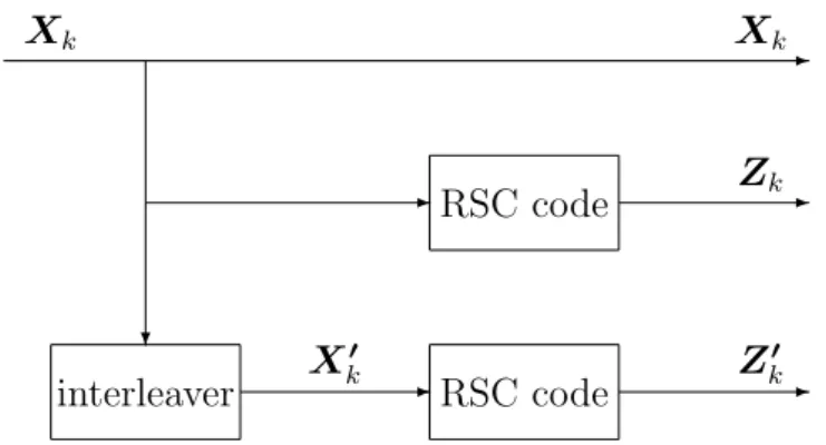
For this reason, we examine in Figure 4.2 the so-called cumulative distance function (CDF) of the codes simulated in Figure 4.1. The y-axis in Figure 4.2 indicates the cumulative number of codeword pairs whose non-coherent distance is below the quantity indicated by the x-axis.

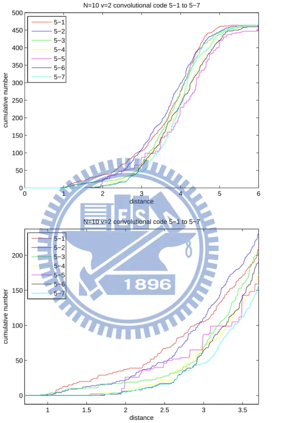
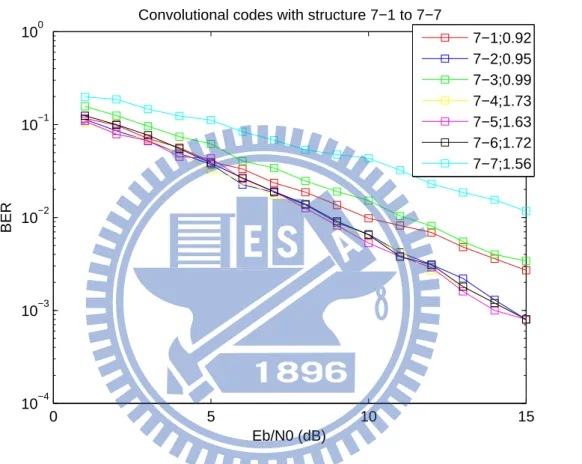
For a more well-rounded understanding of the relation between the CDFs of non-coherent convolutional codes and their performances, another set of convolutional codes is tested. The codes are structured as

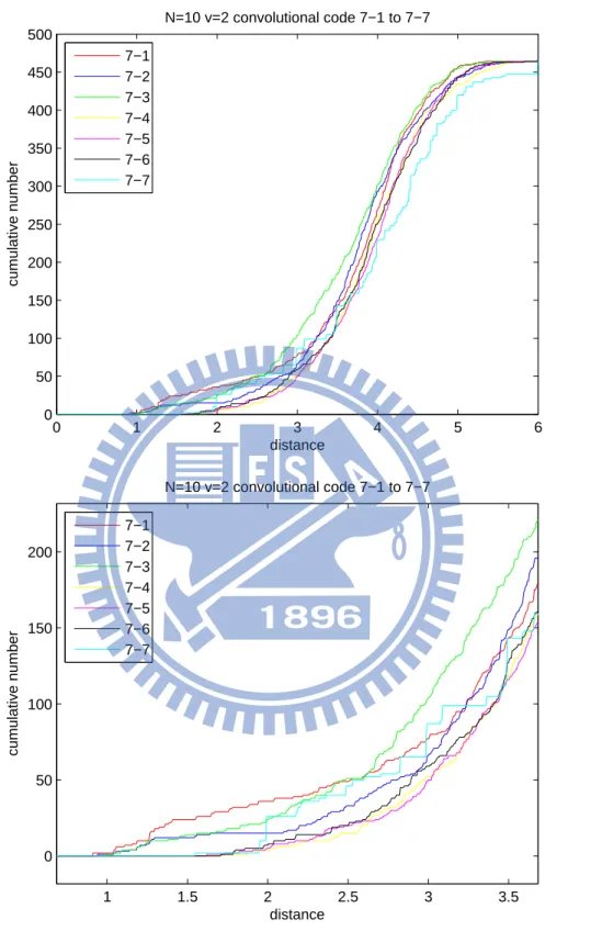
[ 1 + D + D2 D2 ] , . . ., [ 1 + D + D2 1 + D + D2 ] , which are marked as “7-1”, . . . “7-7” in the legends of the respective figures. The results are summarized in Figures 4.3 and 4.4. Same notations, for example, “7-1;0.92”, are used in these two figures. With the CDFs, we can locate good convolutional codes (termed type 1, type 2 and type 3 in Section 3.2.2) using the approach proposed in the previous chapter.

As previously mentioned, the convolutional code that we design is used as an inner code to combat the channel fading. An outer code such as the turbo code will be concate-nated with it. Thus, our next focus is to examine the system performance of the proposed concatenated coding system. Three turbo codes are tested. They are the (37, 21) turbo code [7], the 3GPP/LTE specified turbo code [12], and the turbo code with generator matrix [

1 (1 + D + D2+ D4)/(1 + D3+ D4) ]

[11]. The results for these three turbo codes are respectively illustrated in Figures 4.5–4.7.

Finally, Figures 4.8, 4.9 and 4.10 show the performances of a traditional system struc-ture that replaces our non-coherent inner convolutional code with a least square channel estimators. In these figures, “H′” means the estimated channel matrix by the LS channel

0 5 10 15 10−3 10−2 10−1 100 Eb/N0 (dB) BER

Convolutional codes with structure 5−1 to 5−7

5−1;0.94 5−2;0.94 5−3;1.01 5−4;1.02 5−5;1.16 5−6;0.75 5−7;0.97

Figure 4.1: Performances of non-coherent convolutional codes under blind fading channels. Here, the codeword length N = 10 and the channel memory order is ν = 2. The code rate is 1/2.

0 1 2 3 4 5 6 0 50 100 150 200 250 300 350 400 450 500 distance cumulative number N=10 v=2 convolutional code 5−1 to 5−7 5−1 5−2 5−3 5−4 5−5 5−6 5−7 1 1.5 2 2.5 3 3.5 0 50 100 150 200 distance cumulative number N=10 v=2 convolutional code 5−1 to 5−7 5−1 5−2 5−3 5−4 5−5 5−6 5−7

Figure 4.2: Cumulative distance function (CDF) of the convolutional codes under test. Here, we provide two plots that have different x-axis ranges to facilitate our interpretation of the results. The code rate is 1/2.

0 5 10 15 10−4 10−3 10−2 10−1 100 Eb/N0 (dB) BER

Convolutional codes with structure 7−1 to 7−7

7−1;0.92 7−2;0.95 7−3;0.99 7−4;1.73 7−5;1.63 7−6;1.72 7−7;1.56

Figure 4.3: Performances of non-coherent convolutional codes under blind fading channels. Here, the codeword length N = 10 and the channel memory order is ν = 2. The code rate is 1/2.

0 1 2 3 4 5 6 0 50 100 150 200 250 300 350 400 450 500 distance cumulative number N=10 v=2 convolutional code 7−1 to 7−7 7−1 7−2 7−3 7−4 7−5 7−6 7−7 1 1.5 2 2.5 3 3.5 0 50 100 150 200 distance cumulative number N=10 v=2 convolutional code 7−1 to 7−7 7−1 7−2 7−3 7−4 7−5 7−6 7−7

Figure 4.4: Cumulative distance function (CDF) of the convolutional codes under test. Here, we provide two plots that have different x-axis ranges to facilitate our interpretation of the results. The code rate is 1/2.

8 8.5 9 9.5 10 10.5 10−4 10−3 10−2 10−1 100 Eb/N0 (dB) BER

(37,21) turbo code with type 1, 2 and 3 convolutional codes

type1 type2 type3

Figure 4.5: Performances of the concatenated coding system. The turbo code used is the (37, 21) code proposed by Berrou and Glavieux in [7]. The codeword lengths of the type 1, 2 and 3 convolutional codes are ten, eight and six, respectively. The inner convolutional code rate is 2/3 and the outer turbo code rate is 1/3.

8 8.5 9 9.5 10 10.5 10−4 10−3 10−2 10−1 100 Eb/N0 (dB) BER

3GPP/LTE specified turbo code with type 1, 2 and 3 convolutional codes type1 type2 type3

Figure 4.6: Performances of the concatenated coding system. The turbo code used is the one specified in 3GPP/LTE. The codeword lengths of the type 1, 2 and 3 convolutional codes are ten, eight and six, respectively. The inner convolutional code rate is 2/3 and the outer turbo code rate is 1/3.

8 8.5 9 9.5 10 10.5 11 10−4 10−3 10−2 10−1 100 Eb/N0 (dB) BER

Turbo code in Shu Lin’s book with type 1, 2 and 3 convolutional codes type1 type2 type3

Figure 4.7: Performances of the concatenated coding system. The turbo code used is the one specified in [11]. The codeword lengths of the type 1, 2 and 3 convolutional codes are ten, eight and six, respectively. The inner convolutional code rate is 2/3 and the outer turbo code rate is 1/3.

8 9 10 11 12 13 14 15 10−4 10−3 10−2 10−1 100 Eb/N0 (dB) BER

(37,21) turbo code with convolutional codes and a LS channel estimator type1 type2 type3 type1 with H’ type2 with H’ type3 with H’

Figure 4.8: Performances of a conventional system that employs the (37, 21) turbo code [7] with a least square (LS) channel estimator instead of our non-coherent convolutional code. Here, type 1, type 2 and type 3 similarly denote the sizes of the LS estimator, i.e., 10, 8 and 6. The inner LS channel estimator rate is 2/3 and the outer turbo code rate is 1/3. The curves in Figure 4.5 are also illustrated for comparison.

8 9 10 11 12 13 14 15 16 10−4 10−3 10−2 10−1 100 Eb/N0 (dB) BER

3GPP/LTE specified turbo code with convolutional codes and a LS channel estimator type1 type2 type3 type1 with H’ type2 with H’ type3 with H’

Figure 4.9: Performances of a conventional system that employs the 3GPP/LTE specified turbo code [12] with a least square (LS) channel estimator instead of our non-coherent convolutional code. Here, type 1, type 2 and type 3 similarly denote the sizes of the LS estimator, i.e., 10, 8 and 6. The inner LS channel estimator rate is 2/3 and the outer turbo code rate is 1/3. The curves in Figure 4.6 are also illustrated for comparison.

8 9 10 11 12 13 14 15 16 10−4 10−3 10−2 10−1 100 Eb/N0 (dB) BER

Shu Lin’s turbo code with convolutional codes and a LS channel estimator type1 type2 type3 type1 with H’ type2 with H’ type3 with H’

Figure 4.10: Performances of a conventional system that employs the turbo code from [11] with a least square (LS) channel estimator instead of our non-coherent convolutional code. Here, type 1, type 2 and type 3 similarly denote the sizes of the LS estimator, i.e., 10, 8 and 6. The inner LS channel estimator rate is 2/3 and the outer turbo code rate is 1/3. The curves in Figure 4.7 are also illustrated for comparison.

4.2

Remarks

In this subsection, we will remark on the simulation results presented in the previous sub-section.

As having been pointed out, we can observe from Figures 4.1 and 4.3 that the minimum pairwise non-coherent distance does not seem to be a decisive factor for codes’ performances. On the one hand, Figure 4.1 hints that the code with the largest minimum pairwise non-coherent distance, i.e., “5-5”, gives the worst performance. On the other hand, Figure 4.3 shows the opposite as the code with larger minimum pairwise non-coherent distances usually perform better. A better criterion that can well-connect the pairwise non-coherent distances and the codes’ performances should be adopted. So we turn to the so-called cumulative distance function, based on which the method to select non-coherent convolutional codes is proposed (see (3.2)).

We then apply the convolutional code selection method defined in (3.2) for different codeword lengths, varying from N = 6 to N = 12. The selection results, together with the simulated optimal designs, are listed in Table 4.1. Notably, it is sometimes hard to identify the optimal code design from simulations because their performance curves are close to each other, and one code may outperform the other code in one region but worse in the other region. If such occurs, we will list two or even three as the optimal code designs. There however exist certain code designs that exhibit “strange” CDF patterns like “5-5” and “7-7”, of which the performances are very bad. Particularly, these two codes have many sudden increases in their CDFs.

Next, from Figures 4.5, 4.6 and 4.7, we observed that type 1 code always perform the worst among the tested three types, which seems to hint that our design favors a shorter code. However, there is no apparent winner between type 2 and type 3 codes. To be specific, type

Table 4.1: Convolutional codes identified by the proposed method in (3.2) and the optimal convolutional code designs obtained from simulations. The codeword lengths vary from N = 6 to N = 12. The code rate is 1/2.

type codeword length code selected optimal code

3 N = 6 7-5 5-6 or 7-5

2 N = 8 5-6 4-7 or 5-6 or 7-5

1 N = 10 7-4 7-4

0 N = 12 7-4 5-7 or 7-4 or 7-5

Table 4.2: Convolutional codes identified by the proposed method in (3.2). The codeword lengths vary from N = 6 to N = 12. The code rate is 2/3. Since there are many choices for rate 2/3 codes, to identify the optimal code structures via simulations turns out to be infeasible. Hence, we did not show the optimal code design in this table.

type codeword length code selected

3 N = 6 7-6; 7-5

2 N = 8 5-6; 7-5

1 N = 10 5-6; 7-5

0 N = 12 7-5; 7-6

2 code performs better than type 3 code when they are concatenated with the 3GPP/LTE specified turbo code; however, the winner changes when they are concatenated with the (37, 21) turbo code and the turbo code in [11].

Although we infer that the concatenated coding system that we propose favors a shorter non-coherent convolutional code, the results on type 2 and 3 codes do not support this inference. Hence, we conduct another set of simulations by adding type 0 code, of which the codeword length is 12.

As such, in this series of simulations, four types of codeword lengths are used. They are type 0, type 1, type 2 and type 3, which respectively correspond to codeword lengths 12, 10, 8 and 6. The results are summarized in Figures 4.11, 4.12 and 4.13. These simulations then clearly show that the longest code, i.e., type 0, has the worst performance. However, by

following this trend, type 3 code should always have the best performance but it sometimes performs worse than the type 2 code. An possible cause could be that the the code selected by our method may not be the one with the optimal performance.

In order to verity this interpretation, we additionally perform the following simulations. We replace the non-coherent convolutional codes selected by our method with the optimal non-coherent convolutional codes obtained from simulations. The simulation results are illustrated in Figures 4.14, 4.15 and 4.16. Here, we only focus on codes of lengths 6 and 8. These figures clearly indicate that the shorter type 3 codes are always superior than the longer type 2 codes, thereby confirming our interpretation.

Finally, we remark from Figures 4.8, 4.9 and 4.10 that the performances using our non-coherent convolutional code together with the turbo code are seemingly better than using the LS estimators with the same turbo code. This implies that when the estimation window size of the LS estimator is short such as 6 and 8, it may be advantageous to consider replacing the conventional LS estimator with our non-coherent convolutional code.

8 8.5 9 9.5 10 10.5 11 11.5 10−4 10−3 10−2 10−1 100 Eb/N0 (dB) BER

(37,21) turbo code with type 0, 1, 2 and 3 convolutional codes type 0 type 1 type 2 type 3

Figure 4.11: Performances of the concatenated system that employs the (37, 21) turbo code [7] concatenated with the non-coherent convolutional codes of type 0, 1, 2, 3. Here, the codeword lengths at type 0, 1, 2, 3 codes are respectively 12, 10, 8 and 6. The inner convolutional code rate is 2/3 and the outer turbo code rate is 1/3

8 8.5 9 9.5 10 10.5 11 11.5 10−4 10−3 10−2 10−1 100 Eb/N0 (dB) BER

3GPP/LTE specified turbo code with type 0, 1, 2 and 3 convolutopnal codes type 0 type 1 type 2 type 3

Figure 4.12: Performances of the concatenated system that employs the 3GPP/LTE specified turbo code [12] concatenated with the non-coherent convolutional codes of type 0, 1, 2, 3. Here, the codeword lengths at type 0, 1, 2, 3 codes are respectively 12, 10, 8 and 6. The inner convolutional code rate is 2/3 and the outer turbo code rate is 1/3

8 8.5 9 9.5 10 10.5 11 11.5 10−4 10−3 10−2 10−1 100 Eb/N0 (dB) BER

Shu Lin’s turbo code with type 0, 1, 2 and 3 convolutional codes type 0 type 1 type 2 type 3

Figure 4.13: Performances of the concatenated system that employs the turbo code from [11] concatenated with the non-coherent convolutional codes of type 0, 1, 2, 3. Here, the codeword lengths at type 0, 1, 2, 3 codes are respectively 12, 10, 8 and 6. The inner convolutional code rate is 2/3 and the outer turbo code rate is 1/3

6 6.2 6.4 6.6 6.8 7 7.2 7.4 7.6 7.8 8 10−4 10−3 10−2 10−1 100 Eb/N0 (dB) BER

(37,21) turbo code with the best (2,1) convolutional codes in type 2 and 3 type 2 type 3

Figure 4.14: Performances of the concatenated system that employs the (37, 21) turbo code [7] concatenated with the optimal non-coherent convolutional codes of type 2 and 3. The inner convolutional code rate is 1/2 and the outer turbo code rate is 1/3

6 6.5 7 7.5 8 8.5 10−4 10−3 10−2 10−1 100 Eb/N0 (dB) BER

3GPP/LTE specified turbo code with the best (2,1) convolutional codes in type 2 and 3 type 2 type 3

Figure 4.15: Performances of the concatenated system that employs the 3GPP/LTE specified turbo code [12] concatenated with the optimal non-coherent convolutional codes of type 2 and 3. The inner convolutional code rate is 1/2 and the outer turbo code rate is 1/3

6 6.5 7 7.5 8 8.5 10−4 10−3 10−2 10−1 100 Eb/N0 (dB) BER

Shu Lin’s turbo code with the best (2,1) convolutional codes in type 2 and 3 type 2 type 3

Figure 4.16: Performances of the concatenated system that employs the turbo code from [11] concatenated with the optimal non-coherent convolutional codes of type 2 and 3. The inner convolutional code rate is 1/2 and the outer turbo code rate is 1/3

Chapter 5

Conclusion and Future Work

In this thesis, we proposed a simple non-coherent-distance-based method to select a good convolutional code to co-work with the outer turbo code in an unknown frequency-selective fading environment. By using the selected inner non-coherent convolutional code and the corresponding GLRT decoding criterion, a better performance than the conventional LS estimator can be obtained when the codeword length/estimation window size is small. When the code rate is half, the codes that our method locates are the ones with the simulated

optimal performance. When the code rate increases to 2/3, however, our method may

locate the second-best convolutional code structure in the sense of simulated performance. A side observation from our simulations that the proposed concatenated system prefers using a shorter inner convolutional code. This could be due to that in a dynamic fading environment, it may be better to perform frequent channel estimation based on a smaller window and resort the error protection task to the long outer turbo code.

Our experiments hint that when code rates increase, our method may not select the best code in performance. So some modification may be needed when the code rates further increase. This shall be a useful future research direction. In addition, we restrict the modu-lation schemes to BPSK in our design and simumodu-lations. It shall be more practical to extend our design to a higher order modulations like QPSK and 16-QAM.

Bibliography

[1] O. Shayevitz and M. Feder, “Universal decoding for frequency-selective fading channels,” IEEE Trans. Inf. Theory, vol. 51, no. 8, pp. 2770 - 2790, August 2005.

[2] Haris Gacanin, Mika Salmela and Fumiyuki Adachi, “Performance analysis of analog network coding with imperfect channel estimation in a frequency-selective fading chan-nel,” IEEE Trans. Wireless Commun., vol. 11, no. 2, pp.742 - 750, February 2012. [3] Christos Komninakis, Christina Fragouli, Ali H. Sayed and Richard D. Wesell,

“Chan-nel estimation and equalization in fading,” The Thirty-Third Asilomar Conference on Signals, Systems, and Computers, vol. 2, pp. 1159 - 1163, 24-27 October 1999.

[4] Dilip Warrier and Upamanyu Madhow, “Spectrally efficient noncoherent communica-tion,” IEEE Trans. Inf. Theory, vol. 48, no. 3, pp. 651 - 668, March 2002.

[5] Chia-Long Wu, Po-Ning Chen, Yunghsiang S. Han and Ming-Hsin Kao, “Maximum-likelihood priority-first search decodable codes for combined channel estimation and error correction,” IEEE Trans. Inf. Theory, vol. 55, no. 9, pp. 4191 - 4203, September 2009.

[6] T. Chu, “Joint data detection and channel estimation for OFDM systems,” IEEE Trans. Commun., vol. 54, no. 4, pp. 670 - 679, April 2006.

[7] Claude Berrou and Alain Glavieux, “Near optimum error correcting coding and decod-ing: turbo-codes,” IEEE Trans. Commun., vol. 44, no. 10, pp. 1261 - 1271, October 1996.

[8] Jochen Giese and Mikael Skoglund, “Space-time code design for unknown frequency-selective channels,” 2002 IEEE International Conference on Acoustics, Speech, and Sig-nal Processing (ICASSP), vol. 3, pp. III-2413 - III-2416, 13-17 May 2002.

[9] S. M. Kay, Fundamental of Statistical Signal of Processing, vol. 1 : Estimation Theory, Prentice Hall PTR, 1993.

[10] S. M. Kay, Fundamental of Statistical Signal of Processing, vol. 2 : Detection Theory, Prentice Hall PTR, 1998.

[11] S. Lin and D. J. Costello, Error Control Coding, 2nd edition, Prentice Hall, 2004. [12] 3GPP Technical Specification: Group Radio Access Network, Evolved Universal

Ter-restrial Radio Access, Multiplexing and Channel Coding (Release 8), TS 36.212 v8.3.0, May 2007.