使用網路編碼技術做檔案傳輸之效能評估

國

立

交

通

大

學

網路工程研究所

碩

士

論

文

使用網路編碼技術做檔案傳輸之效能評估

Performance Evaluation for File Transfer using Network

Coding

研 究 生：陳大方

指導教授：易志偉 教授

使用網路編碼技術做檔案傳輸之效能評估

Performance Evaluation for File Transfer using Network Coding

研 究 生：陳大方 Student：Ta-Fang Chen

指導教授：易志偉 Advisor：Chih-Wei Yi

國 立 交 通 大 學

網 路 工 程 研 究 所

碩 士 論 文

Submitted to Institute of Network Engineering College of Computer Science

National Chiao Tung University in partial Fulfillment of the Requirements

for the Degree of Master

in

Computer Science October 2009

摘要

Abstract

We propose a UDP-based file transfer protocol using network coding and eval-uate the performance. The designed protocol, which we call PRNC protocol, takes the advantages of UDP and network coding. Packets transmission over UDP reduces the round trip propagation delay and provides more flexibility than transmission over TCP. And with the help of network coding, we send linear combinations instead of original data. When some packets were lost, if the collected linear combinations were sufficient to be solved, we could still get the original data successfully. Since we don’t need to know which packet we exactly lost, some acknowledgements may be saved. The evaluation re-veals that PRNC protocol behaves almost the same with traditional FTP and has almost three times throughput compare to UFTP.

Contents

3 System Implementation 7 3.1 System Architecture . . . 8

3.2 Pseudo-Random Network Coding Algorithm . . . 10

3.2.1 Pseudo-Random Network Coding Library . . . 10

3.2.2 Performance Analysis . . . 20

3.3 Pseudo-Random Network Coding Protocol . . . 21

3.3.2 PRNC Protocol . . . 27 3.3.3 Performance Analysis . . . 33

List of Figures

1.1 Butterfly example . . . 2

3.1 System Architecture . . . 9

3.2 Architecture of peer clients . . . 10

3.3 Fragmentation diagram in GF (28_{) . . . 12}

3.4 PRNC encoding process . . . 15

3.5 PRNC decoding process . . . 18

3.6 state transition diagram for PRNC algorithm . . . 19

3.7 Encoding Time for PRNC algorithm . . . 21

3.8 Decoding Time for PRNC algorithm . . . 21

3.9 Total equations needed to recover the source file . . . 22

3.10 Dependent ratio for PRNC Algorithm . . . 22

3.11 Three scenarios to show how RTT works . . . 24

3.12 Illustration of batch transmission . . . 25

3.14 The architecture for PRNC protocol . . . 28 3.15 The packet formate in PRNC protocol . . . 31 3.16 State transition diagram of the sender in PRNC protocol . . . 32 3.17 State transition diagram of the receiver in PRNC protocol . . 33 3.18 Download time comparison for PRNC protocol, pure FTP and

UFTP . . . 34 3.19 Throughput comparison for PRNC protocol, pure FTP and

Chapter 1

Introduction

1.1

Network coding

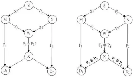
The concept of network coding is first proposed in 2000, and has received extensive attention. The main idea of network coding is to allow coding at the nodes between the source and the receivers. This coding gives the packets some information more than original data. The receivers could use these information to recover the original data or infer the transmission status. First we introduce the famous butterfly example to explain the main idea of network coding. In Fig. 1.1(a), the model does not apply network coding while the model in fig. 1.1(b) uses network coding to transmit packets. The link capacity is one bit per unit time in both models. In order to know how network coding affects, we put the same scenario into both models.

Figure 1.1: Butterfly example

At beginning, the source node generates p1 and p2 and the two packets are

bounded for both D1 and D2. In the model without network coding, we

could easily find that the bottleneck occurs at the intermediate nodes W and

X because the node W can only send one packet. No matter which packet W decides to send first, it still have to transmit the other packet at the next

time. Meanwhile, in the model with network coding, the node W calculate

p1 ⊕ p2 and send the result to the X. When the node D1 received p1 ⊕ p2

from X, it could get p2 by calculating p1⊕ (p1⊕ p2). The node D2 could get

p1 using the same method. Therefor, the average throughput in the model

with network coding is 2 data bits per unit time while it is only 3

2 without

1.2

Motivation

With the previous study in network coding, we observed that there are bene-fits if network coding implemented over UDP but merely mentioned in above works. Therefore, we tried hard to find the way to put network coding into UDP and BT system. Finally, we developed the PRNC algorithm and PRNC protocol. And we found the solution to cowork between PRNC protocol and exist Bittorrent protocol. There are two main benefits in our proposed solu-tion:

1. Less coding overhead compare to linear network coding

2. Less round trip delay and ACK compare to TCP

The use of pseudo-random number reduce the coefficients overhead in linear network coding. Since the overhead is possibly larger than the original data while the coding segment is large, the linear network coding is hard to be used in real system. Therefore, use pseudo-random number to replace the co-efficients greatly reduce the overhead. Another benefit is the round trip delay and times of ACK are reduced. We use the characteristic of network coding to mix data into UDP packets with the same sequence number. Therefore, the receiver only have to send one ACK for one segment and we have less ACK times.

1.3

Organization

In the next chapter, we introduce the related work. The development of net-work coding would be introduced here. And in the third chapter, the main idea and implement would be detailed. The system architecture, PRNC algorithm and PRNC protocol are described in this chapter. Also, the per-formance evaluation results are in the third chapter. Finally we conclude in the fourth chapter.

Chapter 2

Related Work

2.1

Network Coding Development

The concept of ’network coding’ is first proposed by Ahlswede et al [1]. The authors introduce a new class problems which is called network information flow. Their research reveals that if network coding is employed at the node, the bandwidth could be saved.

In [2] and [3], they present a algebraic methods for network coding. The packets transmitted could be seen as one linear combination. Receiver could collect different linear combination from other nodes. Once the receiver get sufficient linear combinations, it could recover the original data by solving the linear equations. They show the surprising result when a multicast con-nection is achievable under different failure scenarios.

In [4], the authors proposed a novel approach called randomized coding. It provides robust, distributed transmission and compression of information. They give a lower bound for success probability andalso the upper bound on failure probability.

In [5], the authors’ research focus on the performance of network cod-ing when the network has dynamic node arrival and departure patterns. Their demonstration shows that network coding mechanism could improve the download time by more than 2-3 times compared to the one without network coding.

Chapter 3

System Implementation

With the previous study in network coding, we have found a novel idea about network coding over P2P network. In order to see how practice our idea is, we put this idea into real system. Our implementation system is based on the BitTorrent architecture which includes tracker server and peer clients. Every component in our system plays the same role in the BitTorrent archi-tecture. Besides the ’data transmission’, the whole behaviors in our system are the same with the ones in BitTorrent. Our network coding mechanism could facilitate the data transmission and data distribution. In this chapter, the system architecture would be depicted first. And in the next section, the Pseudo-random network coding algorithm would be described in detail. Finally, the PRNC protocol which provide reliability for data transfer over UDP would be discussed here.

3.1

System Architecture

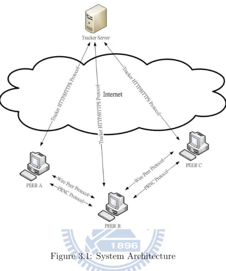
In our implement system, there is one tracker server and three peer clients. The torrent files are stored in all peer clients in advance, thus the HTTP server could be omitted here. Figure 3.1 shows our system architecture. When a peer client starts downloading, it sends request and communicates with the tracker server via Tracker HTTP/HTTPS protocol. After commu-nicating with the tracker server, the client could get a list of peers. Notice that the seed server is always in the list of peers. Then the peer client would send a handshake message to the seed server to build up the tunnel. All messages used in Wire Peer Protocol are exchanged in this TCP tunnel. But unlike original Bittorrent client, our peer client transmit data over UDP tun-nel instead of TCP tuntun-nel. Clients use Wire Peer Protocol to control the whole process and use PRNC Protocol to transmit data.

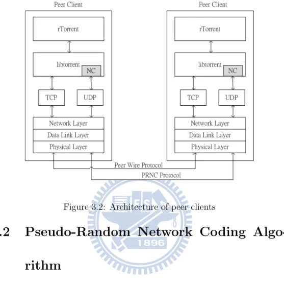
Assume there is one peer client start downloading and get the list of peers in which the seed server is the only one candidate. In this situation, the P2P network could be simplified as a point-to-point network. This help us to understand what we have done in a peer client. We could see the peer client architecture in Figure 3.2. In the top layer, the rTorrent is an BT client application which provides interface for users to control process. The rTorrent uses the library which called libtorrent. We created a new entity in

Figure 3.1: System Architecture

libtorrent which called NC. Our main algorithm PRNC is implemented here. While the libtorrent received a request for sending pieces via TCP tunnel, the NC would create an UDP tunnel, encode raw data and transmit encoded packages via PRNC Protocol. Messages in Peer Wire Protocol are sent via TCP and coded data are sent in UDP.

In the next section, we will introduce the algorithm used in the entity NC. And the PRNC Protocol would be described in the third section.

Figure 3.2: Architecture of peer clients

3.2

Pseudo-Random Network Coding

Algo-rithm

3.2.1

Pseudo-Random Network Coding Library

To the purpose of putting network coding mechanism into real system. We spend efforts on building network coding library which provides flexibility for any other applications. And in order to make network coding more practical, we develop a new approach called PRNC. The main idea in PRNC is using random seed instead of random numbers. In the traditional linear network

overhead is constant. This minimizes the overhead and greatly improves the efficiency. In the following contents, we will introduce the PRNC algorithm and our implemented library in detail.

Notation Definition

Now we are going to present our main idea. Before the discussion of our algorithm, there are some notations needed to be introduced in advance. These notations are described below:

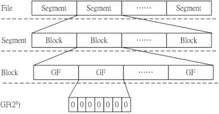
• File: The original data. A File can be fragmented into coding segments.

Notice that in the last segment, the left data size is merely match the fragment size. In this case, the left space in the fragment will filled with zeros.

• Segment: One coding segment consists of blocks. The size of segment

equals to the number of blocks. This implies the number of independent equations needed to recover the original data when decoding.

• Block: One block represents a variable in linear system. In order to

do calculation in Galois Field, one block is fragmented into number of GF. The size of one block equals to the number of GF.

• GF: The size of one GF equals to w in GF (2). For example, the size

Figure 3.3: Fragmentation diagram in GF (28₎

• PRN: PRN means pseudo-random number. It is a random seed used

to generate coefficients in GF.

• B: B is the matrix which represents one segment. Each row in B

represent one block and the number of rows equals to the size of one segment. Every entity in B is a value in GF. Therefore the number of columns equals to the size of one block.

• C: C is the square matrix which represents the coefficients. Every

entity in C is a value in GF and is generated by PRN. The number of rows equals to the segment size.

• E: E is the matrix which represents the encoded data. The number of

rows and columns are the same as B.

have to take care about these notations, especially for the notation segment and the notation block. The segment can be taken as a list of variables and can be represented as B = {B0, B1, ..., Bn} where n is the segment size.

While the block also implies a variable Bi in B and can be represented as

Bi = {Bi,0, Bi,1, ..., Bi,k} where k is the block size.

PRNC Algorithm

Here we are going to introduce the PRNC algorithm. First we will talk about the steps in encoding and then explain how decoding works. And finally the whole procedure of PRNC algorithm would be depicted.

When we are going to encode one segment, the raw data in this segment would be fragmented and saved as B. Each element in the matrix B is a GF and the elements in the same row compose one block. Assume that the segment size is n and the block size is k, the matrix B can be represented as following: B =                 B0,0 · · · B0,k B1,0 · · · B1,k B2,0 · · · B2,k ... . .. ... Bn,0 · · · Bn,k                

Field we use. If we use GF (28_{), the size of B}

i,j is 8 bits (1 byte). And if we

use GF (232_{), the size is 32 bits (4 bytes). The choice of Galois Field degree}

will affect the fragmentation, computing complexity and decode probability. What Galois Field degree we should use depends on what we are focus on. If we want nearly 100% decode probability, according to the previous study(city large scale...), GF (216_{) is the best. If we prefer high computing speed, GF (2}8₎

is absolute the best.

In order to explain how fragmentation works in practical, here is an exam-ple. Assume that we want to fragment this file with segment size 10 and block size 5 in GF (28_{). First, we know the size of GF is 1 byte in GF (2}8_{). Then}

the size of one block is 5 byes and the segment size is 50 bytes. Therefore we could get the matrix B as

B =         B0,0 · · · B0,4 ... ... ... B9,0 · · · B9,4        

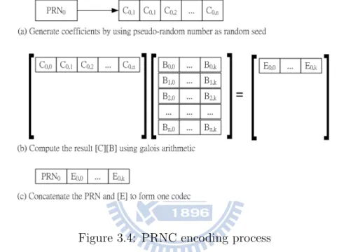
After fragmentation, we pick up a random number PRN. PRN plays a random seed to generate series of random numbers. We call these random numbers as coefficients. The coefficients are values in Galois Field and are saved in the matrix C. Next, we use the matrix multiplication to calculate C × B and save the result in E . Finally, we concatenate the PRN and the

to generate one codec. Notice that one PRN could only generate one codec. Each codec can be taken as a linear equation. In the linear system, we needs n independent equations to solve n variables. Therefore, to completely decode, we needs at leat n PRN and generate at leat n codec.

Figure 3.4: PRNC encoding process

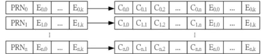
When we collect sufficient independent codec, we could start decoding to get the original data. First, the coefficients in each codec are recovered by PRN. Because we use the same random function, the new coefficients gener-ated in decoding process are the same with the ones genergener-ated in encoding process. As Figure shows below , all codec are merged into the combinational matrix C|E.

            C0,0 C0,1 C0,2 · · · C0,n E0,0 · · · E0,k C1,0 C1,1 C1,2 · · · C1,n E1,0 · · · E1,k ... ... ... ... ... ... . .. ... Cn,0 Cn,1 Cn,2 · · · Cn,n En,0 · · · En,k            

Now it is a traditional linear system problem. But we are not going to solve this directly. There are two phase in decoding process. In the first phase, the matrix C|E is eliminated into a upper triangle matrix. Then we will check the dependency in the upper triangle matrix C0_|E0_{. If there is any}

dependent equation, the linear system can’t be solved. Therefore we have to wait until new codec arrived and makes the whole equations are independent.

            1 C0 0,1 C0,20 · · · C0,n0 E0,00 · · · E0,k0 0 1 C0 1,2 · · · C1,n0 E1,00 · · · E1,k0 ... ... ... ... ... ... . .. ... 0 0 0 · · · 1 E0 n,0 · · · En,k0            

If all linear equations are independent, we start to do the second phase. In the second phase, we solve this linear system by reduce the rows bottom-up. The matrix C0_|E0 _{would be reduced to I|E}00_{. The right matrix E}00 _{is the}

            1 0 0 · · · 0 E00 0,0 · · · E0,k00 0 1 0 · · · 0 E00 1,0 · · · E1,k00 ... ... ... ... ... ... . .. ... 0 0 0 · · · 1 E00 n,0 · · · En,k00            

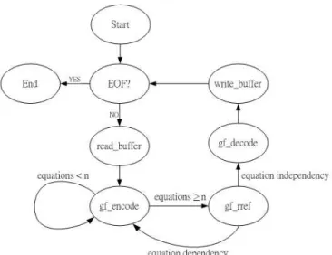
The idea of PRNC algorithm is described in detail above. To better understand our algorithm and the library functions which we are going to introduce, here is a state transition diagram. This diagram depicts the whole process in encoding and decoding. Moreover, the related functions are shown in this diagram. Notice that this diagram only explain how our library works in PRNC algorithm. It is meaningless for a host to encode one file and then decode in real system. But this program could do some performance analysis with different parameters such as degree of Galois Field, segment size block size and etc. Here, we only describe the procedure in this diagram.

When program starts, it begin reading original files and retrieving one segment. Then the segment is fragmented and saved in the double array. The program generates codec continuously until the number of codec is larger or equal to the segment size n. When the number of codec is larger or equal to n, the program does the first phase in decoding. If there is dependency happened, the state transits to gf encode. Then the program would generate a new codec and replace the dependent codec. The loop will continue until

Figure 3.5: PRNC decoding process

the codec are independent. Once all codec are sufficient and independent, the program can decode these codec and transit the state to gf decode. After all, the recovered data would be written into new file. The procedure is keep working until the EOF which means the end of file. Notice that there need some special handle in the tail of the file. Because the last part of one file is merely equals to the size of one segment. In this case, we fill zero into these empty part and only write the valid data.

Figure 3.6: state transition diagram for PRNC algorithm

PRNC Encoding Methods

• gf read buffer(): Read one segment from file and store in buffer. • gf random(): Randomly create one PRN and generate coefficients by

using this PRN as random seed.

• gf encode(): Using matrix multiple in Galois field to encode one

seg-ment.

PRNC Decoding Methods

• gf random(): Randomly create one PRN and generate coefficients by

using this PRN as random seed.

system.

• gf decode(): If the linear system is independent, the function gf decode

is called and the original data would be recover.

• gf write buffer(): Write the segment stored in buffer into file.

3.2.2

Performance Analysis

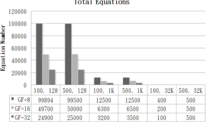
In order to know how the parameters affect the calculate efficiency, we write programs to test the performance. These programs are written in C and we run the programs on the computer with Intel(R) Core(TM)2 Duo CPU 2.1GHz. The size of our target file is 13.5KB. Our interested metrics are the encoding time, decoding time, equations needed and dependent ratio. We analyze these metrics in different Galois Field degree, block size and segment size. The results are shown below. According to these results, in order to achieve best performance, the segment size should be set as 100 and the Galois Field degree should be set as 16. The block size doesn’t affect much when Galois Field degree equals to 16 and the dependent ratio is nearly equals to zero.

Figure 3.7: Encoding Time for PRNC algorithm

Figure 3.8: Decoding Time for PRNC algorithm

3.3

Pseudo-Random Network Coding

Proto-col

In this section we introduce the PRNC protocol. The first subsection de-scribes the reliable approach for UDP transmission. In this issue, we use Jacobson/Karels algorithm as our adaptive retransmission algorithm and the

Figure 3.9: Total equations needed to recover the source file

Figure 3.10: Dependent ratio for PRNC Algorithm

batch mechanism to provide flow control. In the next subsection, the detail of PRNC protocol would be introduced. With the help of PRNC protocol, the transmission delay and network coding overhead could be reduced.

3.3.1

Reliable Approach for UDP Transmission

UDP does not implement flow control or reliable/ordered delivery, thus we need to do a little more work to ensure the transmission reliability. In our designed protocol, there is two mechanism used for the purpose. One is adap-tive retransmission and another is batch mechanism. The first mechanism handle the situations when packet lost occur and the batch mechanism pro-vide flow control and congestion control. In the following paragraph, there are more detail about these mechanism.

Adaptive Retransmission

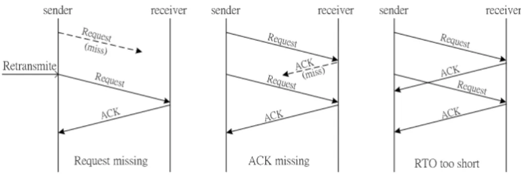
Because the original UDP send packets without reliability, the lost of packet would not be discovered by the both side. In order to handle this problem, the acknowledgement and auto retransmission is required. The choice of retransmission timeout is not easy. If the RTO (Retransmission Timeout) is too large, the retransmission delay time is large when packets lost. If the RTO is too short, the packets redundancy is large so that the bandwidth is occupied by these useless packets.

To overcome these problem, we use Jacobson/Karels algorithm. This is an adaptive retransmission algorithm so that the RTT would change accord-ing to the network situation. To introduce this algorithm, we begin with a

Figure 3.11: Three scenarios to show how RTT works

simple algorithm for computing a timeout value between two host. The host keeps calculate average of the RTT and then to compute the timeout. Every time we send a packet, the time would be recorded and when the ACK for this packet arrives, the arrival time would be saved. We takes the differ-ence between these two times as a SampleRTT. Moreover, we compute an EstimatedRTT as a weighted average. That is,

Dif f erence = SampleRT T − EstimatedRT T EstimatedRT T = EstimatedRT T + (δ × Dif f erence) Diviation = Deviation + δ(|Dif f erence| − Deviation)

where the value δ is between 0 and 1.

Then the timeout value could be computed by the function of Estimate-dRTT and Deviation.

According to the experience, µ is mostly set to 1 and ϕ is set to 4.

Batch Mechanism

To the purpose of maximize the efficiency of packets transmission, we use the batch transmission mechanism. We transmit number of segments first and wait for the ACK. The retransmission would be trigger if the host did not receive the ACK. One batch consists of segments and one segment consists of packets. Packets in the same segment has the same sequence number. With the network coding technique, we do not need to tag different sequence number of the packets in the same segment. Because once we collect sufficient packets (equations), we could recover the original segment sequentially. All we care in one coding segment is the number of independent codec we have. In the other hand, one segment could taken as one super packet.

Figure 3.12: Illustration of batch transmission

While the sender starts to send packets, the batch size is set to be one (it means that one batch contains one segment). The batch size would be increased by one if the NEED in received ACK is zero, that implies no packets

lost. But if the NEED is larger then zero, there must be some packets lost. In this situation, the batch size would not change. And unlike the sliding window protocol for TCP, the batch window would not shift until the whole segments in this batch are transmitted successfully.

Figure 3.13: Example for batch mechanism

For example, if we want to transmit three segments and each segment consist of two packets. At first, only the first segment in the batch window would be send and two encoded packets in the first segment are send. The receiver receives these packets and sends back ACK with NEED = 0 (assume the two encoded packets are independent). The batch size of the sender increase by one because there are no packet lost in the last transmission.

segment and the third segment. All the coded packets in the batch window are send out. But unfortunately the second packet of the third segment is missed. The receiver finds this mistake and send ACK with NEED = 1 after RTO (Retransmission Timeout). The sender keep the second segment and the third segment in the batch window cause there is one packet needed. In this situation, the batch window size would not increase and send one packet in the third segment. After the receiver ACK this segment with NEED = 0, the sender could confirm this transmission is finish.

3.3.2

PRNC Protocol

PRNC protocol puts the PRNC algorithm into real network environment. With the adaptive retransmission and batch mechanism mentioned above, our PRNC algorithm could be applied in UDP. The characteristic of linear network coding gives the advantages of data distribution and data mixing. The flexibility of UDP packet formate helps us to construct the ideal packet regardless of the restrict in TCP packet formate. Therefore, in PRNC proto-col, we choose UDP as our development protocol. The following paragraph describe the PRNC protocol in detail.

System Architecture

The figure below depicts the architecture in one host. One host contains the batch mechanism, PRNC encode and PRNC decode. The host receive codec from other peers via batch mechanism and then use PRNC decode to recover the original data. If there are other peers wants these data, the host use PRNC encode to make codec and transmit to the peers via batch mechanism. Notice that, in the PRNC algorithm, there are two phase for decoding. The host do the first phase if the accumulated codec is larger than the watermark and do the second phase if the result of the first phase is zero, which means the codec is solvable.

Figure 3.14: The architecture for PRNC protocol

Notation Definition

de-• Batch: One batch contains number of segments. The size of the batch

window can be presented as W .

• Segment: One segment represents one coding unit. The size of one

segment is n.

• Codec: The codec is generated from the segment by using PRNC

algo-rithm. The size of one codec is k.

• NEED: The NEED is the number of dependent equations when

decod-ing.

• watermark: The watermark is the point to trigger the PRNC decoding

and can be denoted as w.

• lost rate: The lost rate can be denoted as lt and can be calculated by NEED/RT T .

Packet Formate

The packet format for PRNC protocol are described here. There are two kind of UDP packets through the PRNC protocol. For the codec packet, besides the basic UDP header which includes source port, destination port, length and checksum, there are three header in this format: SegmentID, Timestamp and PRN. The SegmentID identify one packet’s segment. It is

very important that we do not use sequence number to identify every packet. In TCP, it is necessary to identify every packet so that it can reconstruct the original data sequentially. In PRNC protocol, there is no need to record every packet. Instead, it records the segments. And the timestamp attribute is to provide adaptive retransmission. Finally, the PRN attribute is used for PRNC decoding. The last part in one codec packet is the coded data, which can be calculated by the PRNC encoding.

When the receiver get the codec, it would check the number of collected codec. If the codec in the same segment is larger than w, it would start PRNC decoding phase 2. When the segment is recovered or RTT is triggered, the receiver would send ACK back which indicates the NEED. The header of the ACK packet format are SegmentID, Timestamp and NEED. The two former attributes are the same with codec packet. The third attribute implies the number of dependent equations and request for more codec.

State Transition diagram

To illustrate how the PRNC protocol works in one host, there are two state transition diagram for both sender and receiver. In the first diagram, sender initial the batch window and set the next batch. Then we do PRNC encode for all segments in the batch window. There are W × n codec generated at

Figure 3.15: The packet formate in PRNC protocol

After sending out segments, the sender start waiting ACK. If the ACK arrives with NEED = 0, the sender starts preparing the next batch (the batch window size increased by one). But if the ACK arrives with NEED 6= 0, the sender will prepare NEED number of codec to retransmit and wait for the ACK again. If the ACK does not arrive in RTO, we assume the whole codec were missing. In such situation, the sender will prepare W × n codec and send again. The overhead is great when the timeout trigger. Therefore, the adaptive retransmission is very important and we don’t increase the batch window dramatically.

At the side of receiver, first we have to initialize the batch table and set the expect batch window. The packets with different SegmentID would be ignored when arrived. When the first expected packet arrive, the receiver start counting time. If the time is larger than RTO, the ACK with NEED =

Figure 3.16: State transition diagram of the sender in PRNC protocol

n for the segment would be send back. If the number of packets is larger

than watermark w, the receiver start doing PRNC decode phase 1. After row reduce, we could check the codec dependency. If the codec in one segment are determined independent, the receiver could do PRNC decode phase 2 and then send ACK back with NEED = 0. But if there are no sufficient codec or codec dependency is found, the receiver would send ACK back with

NEED = Numberof Dependency. Then go back the stage Receive Packets

Figure 3.17: State transition diagram of the receiver in PRNC protocol

3.3.3

Performance Analysis

In order to know how practical our protocol is, we implement a file transfer program which is build with PRNC protocol. This program is written in C. Our test environment is in WLAN. We compare the performance with FTP and UFTP. The download time and throughput are recorded in dif-ferent file size with size from 100KB to 10MB. According to the result, we found the PRNC protocol has much more performance compare with UFTP and is nearly equals to the FTP. Although network coding mechanism has

some overhead such as computing time, but the transmission time is still the bottleneck. Our batch mechanism could save the times of transmission ACK, since one ACK message is send to acknowledge one segment of pack-ets. Compare to the FTP, the PRNC has better performance in transmitting larger file. The larger file is transmitted, the more packets may be lost. It implies that our PRNC protocol could sustain unreliable environment.

Figure 3.18: Download time comparison for PRNC protocol, pure FTP and UFTP

Figure 3.19: Throughput comparison for PRNC protocol, pure FTP and UFTP

Chapter 4

Conclusion

We proposed the novel idea in network coding and develop PRNC protocol. The PRNC protocol provide better performance compare to the traditional file transfer protocol and also provides security. And it could not only applied in end-to-end file transfer but also peer-to-peer network. We believe that the benefits would be more when it is used in peer-to-peer network. In the future work, we could implement peer-to-peer applications using PRNC protocol and analysis the performance compare to the one without PRNC protocol. These issue are left for anyone interested in.

Bibliography

[1] H. Liu, X. Tu, and J. Xie, “Network coding for p2p live media stream-ing,” in Network and Parallel Computing, 2008. NPC 2008. IFIP

Inter-national Conference on, Oct. 2008, pp. 392–398.

[2] R. Koetter and M. Medard, “Beyond routing: an algebraic approach to network coding,” in INFOCOM 2002. Twenty-First Annual Joint

Conference of the IEEE Computer and Communications Societies. Pro-ceedings. IEEE, vol. 1, 2002, pp. 122–130 vol.1.

[3] S.-Y. Li, R. Yeung, and N. Cai, “Linear network coding,” Information

Theory, IEEE Transactions on, vol. 49, no. 2, pp. 371–381, Feb. 2003.

[4] T. Ho, R. Koetter, M. Medard, D. Karger, and M. Effros, “The benefits of coding over routing in a randomized setting,” in Information Theory,

2003. Proceedings. IEEE International Symposium on, June-4 July 2003,

[5] C. Gkantsidis and P. Rodriguez, “Network coding for large scale con-tent distribution,” in INFOCOM 2005. 24th Annual Joint Conference of

the IEEE Computer and Communications Societies. Proceedings IEEE,

vol. 4, March 2005, pp. 2235–2245 vol. 4.

[6] P. Chou, Y. Wu, and K. Jain, “Practical network coding,” in

Proceedings of the 41st Allerton Conference on Communication, Control, and Computing, September 2003. [Online]. Available: http://citeseerx.ist.psu.edu/viewdoc/summary?doi=10.1.1.11.697

[7] J. MacLaren Walsh and S. Weber, “A concatenated network coding scheme for multimedia transmission,” in Network Coding, Theory and

Applications, 2008. NetCod 2008. Fourth Workshop on, Jan. 2008, pp.

1–6.

[8] D. Nguyen, T. Tran, T. Nguyen, and B. Bose, “Hybrid arq-random network coding for wireless media streaming,” in Communications and

Electronics, 2008. ICCE 2008. Second International Conference on,

June 2008, pp. 115–120.

[9] A. Albanese, J. Blomer, J. Edmonds, M. Luby, and M. Sudan, “Priority encoding transmission,” Information Theory, IEEE Transactions on, vol. 42, no. 6, pp. 1737–1744, Nov 1996.

[10] H. Zeng, J. Huang, S. Tao, and W. Cheng, “A simulation study on net-work coding parameters in p2p content distribution system,” in

Com-munications and Networking in China, 2008. ChinaCom 2008. Third International Conference on, Aug. 2008, pp. 197–201.

[11] R. Bruno, M. Conti, and E. Gregori, “Throughput analysis and mea-surements in ieee 802.11 wlans with tcp and udp traffic flows,” Mobile

Computing, IEEE Transactions on, vol. 7, no. 2, pp. 171–186, Feb. 2008.

[12] M. Wang and B. Li, “Lava: A reality check of network coding in peer-to-peer live streaming,” in INFOCOM 2007. 26th IEEE International

Conference on Computer Communications. IEEE, May 2007, pp. 1082–

1090.

[13] J. Sundararajan, D. Shah, M. Medard, M. Mitzenmacher, and J. Barros, “Network coding meets tcp,” in INFOCOM 2009, IEEE, April 2009, pp. 280–288.

[14] D. Niu and B. Li, “On the resilience-complexity tradeoff of network coding in dynamic p2p networks,” in Quality of Service, 2007 Fifteenth