Analytical and Numerical Analyses of TE-Polarized Waves in the Planar Optical Waveguides with the Nonlinear Guiding Film

Analytical and Numerical Analyses of

TE

-Polarized Waves in the Planar

Optical Waveguides with the Nonlinear Guiding Film

Yaw-Dong Wu* _{and Dong-Heng Cai}

Department of Electronic Engineering

National Kaohsiung University of Applied Sciences, Kaohsiung, 807, Taiwan, R. O. C. FAX: 886-7-3811182, E-mail: ydwu@cc.kuas.edu.tw

Abstract

The modal theory can be used to analyze the wave propagation in the linear and nonlinear planar optical waveguide. By solving the Maxwell's equation and matching the boundary conditions, we can find the eigenmode of transverse electric field in the planar optical waveguide with nonlinear guiding film. A detail modal analysis of the nonlinear waveguide structure is proposed. The analytical results are accompanied by numerical examples. The numerical simulation results show that the analyses are correct.

Keywords : modal theory, Jocabian elliptic function, nonlinear guiding film

1. Introduction

A number of papers have been proposed to discuss the waves propagating along the nonlinear slab optical waveguide structures [1-5]. Considerable progress has been made by considering only Kerr nonlinearities with some additional assumptions. Some of those papers [1-4] that analyze the guiding properties of a nonlinear film have already in the literature. The treatment in Ref. [3] results in the wavenumber of propagation being treated as an implicit function of the modulus of a Jocabian elliptic function.

The modal theory [6-7] can be used to analyze the wave propagation in the linear and nonlinear planar waveguide. By solving the Maxwell's equation and matching the boundary conditions, we can find the eigenmode of transverse electric field in the planar waveguide. We propose an analytical method for analyzing the optical waveguide with the nonlinear guiding film. The numerical simulation results show that our analyses are correct.

2. Analysis

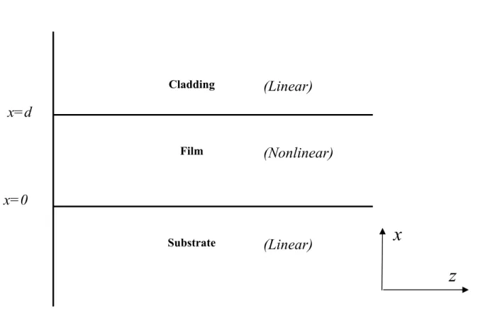
In this paper, we will analytically calculate the TE-polarized waves in the three-layer planar waveguides with the nonlinear guiding film, as shown in Figure 1, and get the exact dispersion relation. The structure is composed of the cladding, the film, and the substrate. The thickness of guiding film is d. The cladding and substrate layers are assumed to extend to infinity in the +x and

-x direction, respectively. The major characteristic of this assumption is that there are no reflections in the x-direction to be concerned with, except for those occurring at interface. For the case of TE plane waves traveling in the z direction, the Maxwell's wave equation can be reduced to

2 2 2 2 2 t c n_{j y} y _∂ ∂ = ∇ ε ε (1)

with solutions of the form

)] ( exp[ ) , ( ) , , (x z t E x z j

β

ω

ε

The subscripts f, c, and s in Eq. (1) are used to denote the guiding film, cladding, and substrate, respectively. For TE waves, the electric field components Ex and Ez are zero. Note also in Eq. (2) that the transverse electric field E(x,z) has no y and z dependence because the planar layers are assumed to be infinite in these directions precluding the possibility of reflections and resultant standing waves. In the following expressions of the field components, the time factor exp(iwt) and the z-dependence exp(-ik0βz) are omitted, where ω is the angular frequency, k0 is the wave number in the free space, and β is the effective refractive index. For Kerr-type nonlinear medium, the square of refractive index of guiding film can be expressed as following:

2 f n = 2 2 ) (x E nfo +α (3)

where n is the linear refractive index of the film and α is the nonlinear coefficient. By _f0 substituting Eq. (2) and Eq. (3) into the wave equation, we can get

0 ) ( ] [ 2 2 2 = −q E x dx d c (4) 0 ) ( ] ) ( [ 2 2 0 2 2 2 = + +q k E x E x dx d f α (5) 0 ) ( ] ) ( [ 2 2 0 2 2 2 = + −Q k E x E x dx d f α (6) 0 ) ( ] [ 2 2 2 = −q E x dx d s (7) where ) ( 2 2 2 0 2 _{= −β} f f k n q , for β <n_f

) ( 2 2 2 0 2 f f k n Q = β − , for β >n_f ) ( 2 2 2 0 2 j j k n q = β − , j = c, s

By solving the differential equations, the transverse electric fields in cladding and substrate can be expressed as follows: )] ( exp[ ) (x E_c p_c x d c = − − ε (8) ] exp[ ) (x E_s p_sx s = ε (9)

where Ec an Es are the values of the electric field at the lower and upper boundaries of the film, respectively. On the other hand, the first integration of Eq. (5) and Eq. (6) gives

) 2 ( ) 2 ( 2 2 2 2 2 0 2 2 2 2 2 0 s f s s c f c c E n n E k E n n E k K = − +α = − +α , (10)

and the second integration gives the electric field in the form

] ) ( [ ) (x bcn A x x₀ l f = + ε (11) ] ' ) ( [ ) ( ' 0 ' '_{cn A x x l} b x f = + ε (12) where 2 1 2 0 2 2 _)] 2 )( [(a b k A= + α , ₂ 2 ₂ b a b l + = , ₂ 0 2 2 0 4 2 2 k q K k q a α α + + = , ₂ 0 2 2 0 4 2 2 k q K k q b α α − + = , 2 1 2 0 2 ' 2 ' ' _)] 2 )( [(a b k A = + α , _{'2 '2} 2 ' ' b a b l + = , ₂ 0 2 2 0 4 2 ' 2 k Q K k Q a α α − + = , 2 0 2 2 0 4 2 ' 2 k Q K k Q b α α + + = ,       = = − b E cn x x ' 1 0 0 0 , 0 x and ' 0

x are the second constants of integration, and cn is a specific Jacobian elliptic function. For simplicity, the modulus l is omitted in the following discussions. Considering the case β <n_f and matching the boundary conditions, we could obtain the following eiqenvalue equation:

−       − −    − − = ( ) ( ){[1 (1 )] ( )(1 ₂ )} 2 2 2 2 b E Ad lcn b E l Ad dn Ad sn b E Ab q E_{c c s s s}

2 2 2 2 2_{( ) ( )]} ( ) ( ) ( ) )[ (           ₊    − b E Ab q E Ad dn Ad sn b E Ad cn Ad lsn b E Ad dn Ad cn Ab q E c s s s s s s ₍₁₂₎

where sn and dn are Jacobi elliptic functions. The Eq. (12) can be solved numerically. When constants β and Es are determined, all the other constants q ,_f q ,_s q , K, A, a, b, l, _c x , and Ec₀ are also determined.

For the case that β >n_f , on the other hand, we just have to replace the constants A, a, b, l, and x in Eq. (12) with _{0 A}', _{a ,} ' _{b ,} ' _{l and} ' '

0

x , and get these equations with similar expressions. When constants β and Es are determined, all the other constants q ,_f q ,_s q , K, _c A',a', b', l', x₀' and Ec are also determined.

The power per unit width along the y-axis carried in the z direction by the nonlinear guided wave is obtained by integrating the Poynting vector and time averaging:

∫

For the linear planar waveguide, the effective refractive index β is independent of the input power. Whereas for the nonlinear planar waveguide, β is dependent on the input power. Since the effective refractive index of the nonlinear waveguide is changed gradually with the intensity of the input light beam, there is an intimate relation between the effective refractive index and power in the nonlinear waveguide. This relation is so-called the dispersion relation. For a nonlinear film, on the other hand, bounded by semi-infinite dielectrics, the electric field outside the film must always decay exponentially at each boundary. Therefore, the electric field inside the film must always increase from the boundary. In this sense, the field always resembles linear guided waves, and this is reinforced by the periodic nature of the Jocabin elliptic functions. Because of this periodicity, an infinite numbers are possible, we only present the TE0, TE1 and TE2 waves here as being sufficient numerical illustrations of the theory and dispersion relations.

3. Numerical Results

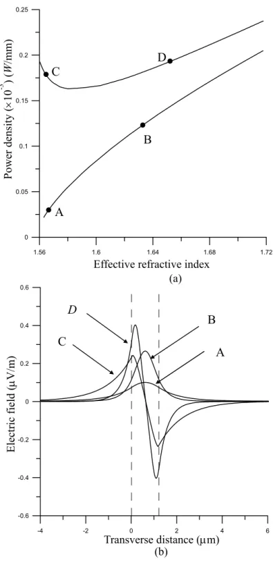
Consider the case that the refractive index of guiding film is higher than the refractive index of cladding and substrate. It means that confined modes are possible when the effective refractive index of the three-layer planar waveguide is higher than the refractive index of cladding and substrate. Several numerical examples are presented as follows. All numerical results presented here were calculated with the values: n_c = =1.55, n_s n_f0 =1.57, _{α =6.3786µm}2_/V2_{, and the free} space wavelength λ=1.3µm. Figure 2(a) shows the dispersion curve of TE0 wave in the three-layer nonlinear waveguide with the width d = 0.8µm of the guiding film. Figure 2(b) shows the electric field distributions for the various input optical power density shown in Figure 2(a). Figure 3(a) shows the dispersion curves of TE0 and TE1 waves in the three-layer nonlinear waveguide with the

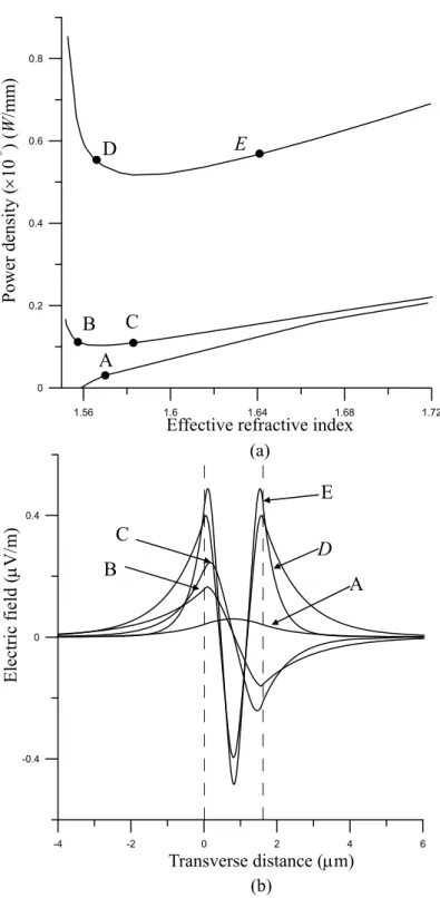
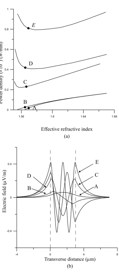
width d = 1.2 µm of the guiding film. Figure 3(b) shows the electric field distributions for the various input optical power density shown in Figure 3(a). Figure 4(a) shows the dispersion curves of TE0, TE1 and TE2 waves in the three-layer nonlinear waveguide with the width d = 1.6 µm of the guiding film. Figure 4(b) shows the electric field distributions for the various input optical power density shown in Figure 4(a). Figure 5(a) shows the dispersion curves of TE0, TE1, TE2, TE3 and TE4 waves in the three-layer nonlinear waveguide with the width d = 3 µm of the guiding film. Figure 5(b) shows the electric field distributions for the various input optical power density shown in Figure 5(a). As shown in Figure 2 to Figure 5, as the guided power increases and consequently β increases, the electric field distributions gradually become narrow, and the optical wave would be confined in the nonlinear film.

4. Conclusions

In this paper, we propose an analytical method for analyzing the optical waveguide with the nonlinear guiding film. We give a detailed modal analysis of the proposed nonlinear waveguide structure. The analytical results are accompanied by numerical examples. The numerical simulation results show that our analyses are correct.

References

[1] Fedyanin, V. K. and D. Mikhalake, “P-polarized Nonlinear Surface Polarized in Layered Structures,” Z. Phys. B, Vol. 47, 1984, pp. 167-181.

[2] Langbern, U., F. Legerer, and H. E. Ponath, “A New Type of Nonlinear Slab-Guided Waves,” Opt. Commun., Vol. 46, 1982, pp. 167-169.

[3] Akhmediev, N. N., K. O. Botar, and V. M. Eleonskii, “Dielectric Optical Waveguide with Nonlinear Susceptibility Symmetric Refractive-Index Profile,” Opt. Spectrum (USSR), Vol. 53(b), 1982, pp. 654-658.

[4] Boardman, A. D. and P. Egan, “Optically Nonlinear Waves in Thin Films,” IEEE J. Quantum Electron, Vol. 22, 1986, pp. 319-324.

[5] Danielsen, P. and D. Yevick, “Improved Analysis of the Propagating Beam Method in Longitudinally Perturbed Optical Waveguides, ”Appl. Opt., Vol. 21, 1982, pp. 4188-4189. [6] Burns, W. K. and A. F. Milton, “Mode Conversion in Planar Dielectric Separating

Waveguides,” IEEE J. Quantum Electron, Vol. 11, 1975, pp. 32-39.

[7] Zutsu, M. I., Y. Nakai, and T. Sutena, “Operation Mechanism of the Single-Mode Optical-Waveguide Y Junction,” Opt. Lett., Vol. 7, 1982, pp. 136-138.

x=d

x=0

(Linear)

(Nonlinear)

(Linear)

x

z

Transverse distance (µm) Electric field (µ v/m) A B C D A B C D

Effective refractive index (a)

Figure 2. (a) The dispersion relation of TE0 wave in a three-layer nonlinear waveguide with d

= 0.8µm. (b) Field distribution at four points A-D in (a).

1.56 1.6 1.64 1.68 1.72 0 0.04 0.08 0.12 0.16 0.2 -8 -4 0 4 8 0 0.1 0.2 0.3 0.4 Power density ( ×10 -3 ) ( W /mm) (b)

A

B C

D

Effective refractive index (a) A B C D Transverse distance (µm) Electric field (µ V/ m)

Figure 3. (a) The dispersion relation of TE0 and TE1 wave in a three-layer nonlinear

waveguide with d = 1.2µm. (b) Field distribution at four points A-D in (a).

1.56 1.6 1.64 1.68 1.72 0 0.05 0.1 0.15 0.2 0.25 -4 -2 0 2 4 6 -0.6 -0.4 -0.2 0 0.2 0.4 0.6 (b) Power density ( ×10 -3 ) ( W /mm)

Transverse distance (µm) (b) Electric field (µ V/ m)

Figure 4. (a) The dispersion relation of TE0, TE1 and TE2 wave in a three-layer nonlinear

waveguide with d=1.6µm. (b) Field distribution at five points A-E in (a).

E A D B C Power density ( ×10 -3 ) ( W /mm)

Effective refractive index (a) A B C D E 1.56 1.6 1.64 1.68 1.72 0 0.2 0.4 0.6 0.8 -4 -2 0 2 4 6 -0.4 0 0.4

A B

C D

E

Effective refractive index (a) Transverse distance (µm) (b) Electric field (µ V/ m)

Figure 5. (a) The dispersion relation of TE0, TE1, TE2, TE3 and TE4 wave in a three-layer

nonlinear waveguide with d = 3µm. (b) Field distribution at five points A-E in (a).

Power density ( ×10 -3 ) ( W /mm) A B C D E 1.56 1.6 1.64 1.68 0 0.2 0.4 0.6 0.8 1 -4 0 4 8 -0.4 0 0.4