Transfer Function Model-Lecture 1

(1)

THE UNIVERSITY OF CHICAGO Booth School of Business

Business 41914, Spring Quarter 2009, Mr. Ruey S. Tsay

Lecture 1: Transfer Function Model

1 Introduction

Transfer function model is a statistical model describing the relationship between an output variable Y and one or more input variables X. It has many applications in business and economics, especially in forecasting turning points. Examples of forecasting applications of the model include assessing the impact of monthly advertisement on the profit of a firm and the effect of monthly average daily temperature on gas bill of a household. In most applications, linear equation is used to describe the relationship, resulting in the distributed-lag model commonly known in the econometric literature. For simplicity, we focus on discrete-time linear models. By discrete-time, we meant that the data are observed at discrete time points, even though the actual process may be continuous in time. The variables Y and X are typically continuous random variables. By linear model, we mean that the relationship between Y and X is linear and both X and Y are linear processes.

Let us start with the simple case that X is a scalar variable and Y has no additional innovation. In this case, the dynamic dependence of Yton the current and past values of the X, namely {Xt−j}∞j=0,

can be written as

Yt = v0Xt+ v1Xt−1+ v2Xt−2+ v3Xt−3+ · · · ,

= v(B)Xt (1)

where v0, v1, · · · are constant denoting the impact of Xt−j on Yt, and v(B) = v0+ v1B + v2B2+ · · ·

with B denoting the backshift operator such that BXt = Xt−1. In the economic literature, lag

operator (L) is often used instead of the notation B. The coefficients v0, v1, · · · are referred to as

the impulse response function of the system.

For the model in Eq. (1) to be meaningful, the impulse responses must satisfy certain condition. A simple condition is that P∞

j=0|vj| < ∞, i.e., the impulse responses are absolutely summable. In

this case, the system is said to be stable. The value g =

∞

X

j=0

vj

is called the steady-state gain as it represents the impact on Y when Xt−j are held constant over

time.

The function v(B) determines the impact of input Xt on output Yt. It pays to study some simple

examples of v(B). See Table 10.6 of Box, Jenkins and Reinsel (1994, p. 389).

Example 1. Consider the model Yt= B3Xt. What is the impulse response function? What is the

(2)

Example 2.Consider the model Yt= (0.5 + 0.5B)B3Xt. What is the impulse response function?

What is the cumulative response function?

Example 3. Consider the model (1 − 0.5B)Yt= 0.5B3Xt. What is the impulse response function?

What is the cumulative response function?

For the model in Eq. (1) to be practical, the number of impulse response coefficients vj must

satisfy certain constraints. For instance, one can use the same idea as the univariate autoregressive integrated moving-average (ARIMA) model to describe the function v(B). That is, one assumes that v(B) is a rational polynomial in B such as

Yt=

ω(B)Bb

δ(B) Xt, (2)

where b is a non-negative integer, ω(B) = ω0+ω1B+ω2B2+· · ·+ωsBsand δ(B) = 1−δ1B−· · ·−δrBr

are finite-order polynomials in B, and ω06= 0. Obviously, ω(B) and δ(B) have no common factors.

The prior model says that v(B) = ω(B)Bb/δ(B).

The parameter b is called the time delay (or dead time) of the system. For example, if b = 1, then v0 = 0 and Xt has no impact on Yt, but Xt will affect Yt+1. In other words, the impact of Xt on

the output series {Yt} is delayed for one time period.

Question: Under what condition that v(B) = ω(B)Bb/δ(B) of Eq. (2) gives rise to a stable transfer function?

Question: Suppose that in Eq. (2) v(B) = ω(B)Bb/δ(B) is stable. What is the steady-state gain of the system?

2 Transfer Function Model

In practice, the output Ytis not a deterministic function of Xt. It is often disturbed by some noise

or has its own dynamic structure. We denote the noise component as Nt. The noise may be serially

correlated, and we assume that Nt follows an ARMA(p, q) model, i.e.

φ(B)Nt= θ(B)at, (3)

where θ(B) = 1 − θ1B − · · · − θqBqand φ(B) = 1 − φ1B − · · · − φpBp are polynomials in B of degree

(3)

variables with mean zero and variance σ2_a. Often we also assume that atis Gaussian. Note that for

the ARMA model in Eq. (3), E(Nt) = 0 and the usual conditions of stationarity and invertibility

apply.

Putting together, we obtain a simple transfer function model as Yt= c + v(B)Xt+ Nt=

ω(B)Bb

δ(B) Xt+ θ(B)

φ(B)at, (4)

where c is a constant, θ(B), φ(B), ω(B) and δ(B) are defined as before with degree q, p, s and r, respectively, and {at} are Gaussian white noise series. The noise component Nt should be

independent of Xt; otherwise, the model is not identifiable.

Note that when b > 0 the transfer function model is useful in predicting the turning points of Yt

given those of Xt.

When there are multiple input variables, say two, the transfer function model becomes Yt= c + ω1(B)Bb1 δ1(B) X1t+ ω2(B)Bb2 δ2(B) X2t+ θ(B) φ(B)at, where ωi(B) and δi(B) are similarly defined as in Eq. (4).

3 An Example

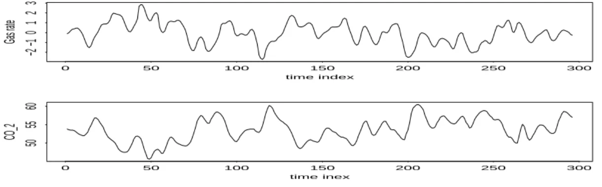
Consider the Gas-Furnace example of Box, Jenkins and Reinsel (1994, Chapter 11). The data consist of 296 observations of (a) input gas rate in cubic feet per minute and (b) the percentage of CO2 in outlet gas. The time interval used is 9 seconds and the actual feed rate is Zt= 0.6 − 0.04Xt,

where Xtis the input series. What is the dynamic relationship between the input gas rate Xt and

the output CO2 measurement Yt? Figure 1 gives the time plot of the data.

Given the data set, our goal is to specify an adequate model for making inference. One approach to achieve this objective is to adopt the iterated modeling procedure of Box and Jenkins (1976) which consists of the following steps:

1. Model specification, 2. Estimation,

3. Model checking (residual analysis).

If a fitted model is judged to be inadequate via model checking statistics, the procedure is iterated to refine the model. A model that passed rigorous model checking can then be used to make inference, e.g. forecasting or policy simulation.

4 Model Building

The task of model specification in the case of a single input variable involves • estimation of the impulse response function v_i’s,

(4)

time index Gas rate 0 50 100 150 200 250 300 −2 −1 0 1 2 3 time inex CO_2 0 50 100 150 200 250 300 50 55 60

Figure 1: Time plots of Input and Output Series: Gas-Furnace Example

• identification of the rational polynomials ω(B) and δ(B) and the delay b to best approximate v(B).

We shall briefly discuss methods and statistics that are useful in specifying a transfer function model.

4.1 Preliminary estimation of v(B)

Consider the TFM in Eq. (4). Since Xt and Nt might be serially dependent, the regression

Yt= c + v0Xt+ v1Xt−1+ · · · + vhXt−h+ et,

where h is a large positive integer, would, in general, not provide consistent estimates of the vi’s.

In the literature, pre-whitening has been proposed as a tool to obtain consistent estimates of vi.

The idea of pre-whitening is to remove the serial dependence in Xt. Suppose that Xt follows the

univariate ARMA model

φx(B)Xt= θx(B)ηt,

where {ηt} is a sequence of white noises (i.e. iid random variables). Applying the operator φ_θ_xx_(B)(B)

to Eq. (4), we obtain φx(B) θx(B) Yt = c∗+ v(B) φx(B) θx(B) Xt+ φx(B) θx(B) Nt = c∗+ v(B)ηt+ φx(B) θx(B) Nt,

(5)

where c∗ is a constant given by c∗= φx(1) θx(1)c. Define yt= φx(B) θx(B) Yt, nt= φx(B) θx(B) Nt.

The prior equation reduces to

yt= c∗+ v(B)ηt+ nt. (5)

Notice that {nt} is independent of {ηt} and ηt is a white noise series. Multiplying Eq. (5) by ηt−j,

for j ≥ 0, we have

ytηt−j = c∗ηt−j+ [v(B)ηt]ηt−j+ ntηt−j.

Taking expectation, we obtain

Cov(yt, ηt−j) = vjVar(ηt−j). Consequently, we have vj = Cov(yt, ηt−j) Var(ηt) . In term of cross-correlation, we have

vj = Corr(yt, ηt−j)

std(yt)

std(ηt)

.

In practice, the model for Xtcan be specified via the univariate time series analysis (e.g., Bus 41910

or Bus 41202). One can then apply the model to obtain yt. This process is called pre-whitening or

filtering in the time series literature.

Discussion: Some comments on pre-whitening are in order.

1. In finite samples, the accuracy of vj estimates might be affected by the noise term nt.

2. Pre-whitening becomes complicated when there are multiple input variables.

4.2 A rough approximation

Experience shows that the effect of Nt on the estimation of v(B) can often be reduced when a

simple model is assumed for Nt. In theory, the resulting estimates of vj are biased. However,

such estimates can often serve the purpose of model specification. The approximate models for Nt

include the following:

• An AR(1) model if Y_tis not a seasonal time series. Here we use the approximate model Nt=

1 1 − φ1B

at.

• A seasonal ARIMA(1,0,0)(1,0,0) model if Y_t is seasonal. Here the approximate model is Nt=

1

(1 − φ1B)(1 − φkBk)

at,

(6)

SCA demonstration: The two methods produce close estimates of vj for the Gas-Furnace data

set.

*** Analysis of Gas-Furnace data ***

--input x,y. file ’gasfur.dat’

X , A 296 BY 1 VARIABLE, IS STORED IN THE WORKSPACE Y , A 296 BY 1 VARIABLE, IS STORED IN THE WORKSPACE

--iarima x.

THE FOLLOWING ANALYSIS IS BASED ON TIME SPAN 1 THRU 296

THE CRITICAL VALUE FOR SIGNIFICANCE TESTS OF ACF AND ESTIMATES IS 1.960 SUMMARY FOR UNIVARIATE TIME SERIES MODEL -- UTSMODEL

---VARIABLE TYPE OF ORIGINAL DIFFERENCING

VARIABLE OR CENTERED

X RANDOM ORIGINAL NONE

---PARAMETER VARIABLE NUM./ FACTOR ORDER CONS- VALUE STD T

LABEL NAME DENOM. TRAINT ERROR VALUE

1 X D-AR 1 1 NONE 1.9755 .0549 36.01

2 X D-AR 1 2 NONE -1.3741 .0994 -13.82

3 X D-AR 1 3 NONE .3430 .0549 6.25

TOTAL NUMBER OF OBSERVATIONS . . . . 296 EFFECTIVE NUMBER OF OBSERVATIONS . . 293 RESIDUAL STANDARD ERROR. . . 0.188754E+00

--tsm mx. model (1,2,3)x=noise.

--estim mx. hold resi(rx)

THE FOLLOWING ANALYSIS IS BASED ON TIME SPAN 1 THRU 296 SUMMARY FOR UNIVARIATE TIME SERIES MODEL -- MX

(7)

1 X AR 1 1 NONE 1.9755 .0549 36.01

2 X AR 1 2 NONE -1.3741 .0994 -13.82

3 X AR 1 3 NONE .3430 .0549 6.25

EFFECTIVE NUMBER OF OBSERVATIONS . . 293 R-SQUARE . . . 0.969 RESIDUAL STANDARD ERROR. . . 0.188754E+00

--filter model mx. old x,y. new eta,fy.

THE FOLLOWING ANALYSIS IS BASED ON TIME SPAN 1 THRU 296 SERIES X IS FILTERED USING MODEL MX, THE RESULT IS IN ETA SERIES Y IS FILTERED USING MODEL MX, THE RESULT IS IN FY

--ccf x,y. maxl 12.

TIME PERIOD ANALYZED . . . 1 TO 296

NAMES OF THE SERIES . . . X Y

EFFECTIVE NUMBER OF OBSERVATIONS . . . 296 296

STANDARD DEVIATION OF THE SERIES . . . 1.0710 3.1967 MEAN OF THE (DIFFERENCED) SERIES . . . -0.0568 53.5091 STANDARD DEVIATION OF THE MEAN . . . . 0.0622 0.1858 T-VALUE OF MEAN (AGAINST ZERO) . . . . -0.9130 287.9856

CORRELATION BETWEEN Y AND X IS -0.48

CROSS CORRELATION BETWEEN X(T) AND Y(T-L)

1- 12 -.39 -.33 -.29 -.26 -.24 -.23 -.21 -.18 -.15 -.12 -.09 -.08 ST.E. .06 .06 .06 .06 .06 .06 .06 .06 .06 .06 .06 .06 CROSS CORRELATION BETWEEN Y(T) AND X(T-L)

1- 12 -.60 -.73 -.84 -.92 -.95 -.91 -.83 -.72 -.60 -.50 -.41 -.35 ST.E. .06 .06 .06 .06 .06 .06 .06 .06 .06 .06 .06 .06 -1.0 -0.8 -0.6 -0.4 -0.2 0.0 0.2 0.4 0.6 0.8 1.0 +----+----+----+----+----+----+----+----+----+----+ I -12 -0.35 XXXXXX+XXI +

(8)

-11 -0.41 XXXXXXX+XXI + -10 -0.50 XXXXXXXXX+XXI + -9 -0.60 XXXXXXXXXXXX+XXI + -8 -0.72 XXXXXXXXXXXXXXX+XXI + -7 -0.83 XXXXXXXXXXXXXXXXXX+XXI + -6 -0.91 XXXXXXXXXXXXXXXXXXXX+XXI + -5 -0.95 XXXXXXXXXXXXXXXXXXXXX+XXI + -4 -0.92 XXXXXXXXXXXXXXXXXXXX+XXI + -3 -0.84 XXXXXXXXXXXXXXXXXX+XXI + -2 -0.73 XXXXXXXXXXXXXXX+XXI + -1 -0.60 XXXXXXXXXXXX+XXI + 0 -0.48 XXXXXXXXX+XXI + 1 -0.39 XXXXXXX+XXI + 2 -0.33 XXXXX+XXI + 3 -0.29 XXXX+XXI + 4 -0.26 XXXX+XXI + 5 -0.24 XXX+XXI + 6 -0.23 XXX+XXI + 7 -0.21 XX+XXI + 8 -0.18 X+XXI + 9 -0.15 X+XXI + 10 -0.12 XXXI + 11 -0.09 +XXI + 12 -0.08 +XXI +

--ccf eta,fy. maxl 12. hold --ccf(vb).

TIME PERIOD ANALYZED . . . 4 TO 296

NAMES OF THE SERIES . . . ETA FY

EFFECTIVE NUMBER OF OBSERVATIONS . . . 293 293

STANDARD DEVIATION OF THE SERIES . . . 0.1887 0.3628 MEAN OF THE (DIFFERENCED) SERIES . . . -0.0038 2.9778 STANDARD DEVIATION OF THE MEAN . . . . 0.0110 0.0212 T-VALUE OF MEAN (AGAINST ZERO) . . . . -0.3479 140.5124

CORRELATION BETWEEN FY AND ETA IS 0.00

CROSS CORRELATION BETWEEN ETA(T) AND FY(T-L)

1- 12 -.03 .01 -.05 -.02 -.00 -.12 -.03 -.09 .00 .02 .01 -.00 ST.E. .06 .06 .06 .06 .06 .06 .06 .06 .06 .06 .06 .06 CROSS CORRELATION BETWEEN FY(T) AND ETA(T-L)

(9)

ST.E. .06 .06 .06 .06 .06 .06 .06 .06 .06 .06 .06 .06 -1.0 -0.8 -0.6 -0.4 -0.2 0.0 0.2 0.4 0.6 0.8 1.0 +----+----+----+----+----+----+----+----+----+----+ I -12 -0.02 + I + -11 -0.03 + XI + -10 -0.05 + XI + -9 0.03 + IX + -8 -0.02 + XI + -7 -0.17 X+XXI + -6 -0.27 XXXX+XXI + -5 -0.46 XXXXXXXX+XXI + -4 -0.33 XXXXX+XXI + -3 -0.28 XXXX+XXI + -2 -0.02 + XI + -1 0.05 + IX + 0 0.00 + I + <=== Lag-0 1 -0.03 + XI +

2 0.01 + I + This part gives info

3 -0.05 + XI + about unidirection.

4 -0.02 + I + Should be also ‘‘zero’’.

5 0.00 + I + 6 -0.12 XXXI + 7 -0.03 + XI + 8 -0.09 +XXI + 9 0.00 + I + 10 0.02 + IX + 11 0.01 + I + 12 0.00 + I + --ff=sqrt(var(fy))/sqrt(var(eta)) --vhat=vb*ff --print vhat VHAT IS A 25 BY 1 VARIABLE -.033 -.063 -.104 .061 -.047 -.322 -.515 -.876 -.635 -.543 -.047 .105 -.002 -.057 .019 -.093 -.030 -.005 -.231 -.049 -.171 .002 .042 .013 -.009

(10)

--estim m1. hold resi(r1)

THE FOLLOWING ANALYSIS IS BASED ON TIME SPAN 1 THRU 296 SUMMARY FOR UNIVARIATE TIME SERIES MODEL -- M1

Y RANDOM ORIGINAL NONE

1 C CNST 1 0 NONE 53.8882 .7899 68.22 2 X NUM. 1 0 NONE -.0482 .0958 -.50 3 X NUM. 1 1 NONE .0987 .1321 .75 4 X NUM. 1 2 NONE -.0345 .1341 -.26 5 X NUM. 1 3 NONE -.5262 .1340 -3.93 6 X NUM. 1 4 NONE -.6371 .1360 -4.69 7 X NUM. 1 5 NONE -.8301 .1360 -6.10 8 X NUM. 1 6 NONE -.4935 .1358 -3.63 9 X NUM. 1 7 NONE -.3267 .1360 -2.40 10 X NUM. 1 8 NONE -.0544 .1359 -.40 11 X NUM. 1 9 NONE .0257 .1340 .19 12 X NUM. 1 10 NONE -.0910 .1340 -.68 13 X NUM. 1 11 NONE -.0598 .1321 -.45 14 X NUM. 1 12 NONE -.0051 .0954 -.05 15 Y D-AR 1 1 NONE .9769 .0216 45.25

--stop <== quit SCA.

4.3 Specification of model for Nt

Construct the estimate of Nt by

ˆ

Nt= Yt− ˆc − ˆv(B)Xt.

Apply the usual univariate time series methods to identify a model for Ntusing ˆNtas the observed

(11)

4.4 Specification of transfer function

The goal is to find a rational form for v(B). To this end, we can use the Corner method, which is based on the Pade approximation of a polynomial. From

v(B) = ω(B)B b δ(B) , we obtain v0+ v1B + v2B2+ · · · = ω0Bb+ ω1Bb+1+ · · · + ωsBb+s 1 − δ1B − · · · − δrBr . By equating the coefficients of Bj, it is easy to see that

• v_j = 0 for j < b if b is positive.

• vb, vb+1, · · · , vb+s−r follow no fixed pattern (no such values occur if s < r),

• v_j with j ≥ b + s − r + 1 follows a rth order difference equation

vj = δ1vj−1+ · · · + δrvj−r, or δ(B)vj = 0, (6)

with starting values vb+s, · · · , vb+s−r+1.

Example. Consider the case ω(B) = ω0 + ω1B + ω2B2, b = 1, and δ(B) = 1 − δ1B. Here

(r, s, b) = (1, 2, 1). We have v0+ v1B + v2B2+ · · · = ω0B + ω1B2+ ω2B3 1 − δ1B . Therefore, v0+ v1B + v2B2+ · · · = (ω0B + ω1B2+ ω2B2)(1 + δ1B + δ21B2+ · · ·).

By equating coefficients, we have • v0 = 0,

• v₁= ω0 and v2 = δ1ω0+ ω1 = δ1v1+ ω1,

• v3= δ12ω0+ δ1ω1+ ω2 = δ1v2+ ω2, (starting value)

• v₄= δ₁3ω0+ δ12ω1+ δ1ω2 = δ1v3, and v5= δ1v4, etc.

The last result can be written as (1 − δ1B)vj = 0 for j ≥ 4 with starting value v3.

In general, any polynomial v(B) can be approximated as accurately as possible by some ratio of two finite-order polynomials by increasing the orders of the two finite-order polynomials. In practice, we seek to find suitable (r, s, b) so that the approximation is adequate. The property that the coefficients vj satisfy a rth order difference equation is used in the Corner Method to specify

(r, s, b).

Corner Method. Corner method is a two-way table designed to show the pattern of vj. The

(12)

u(B) = v(B)/vmax, where vmax = maxj{|vj|}. The (i, j)-th element of the two-way table is the

determinant of the j × j matrix

M (i, j) =       ui ui−1 · · · ui−j+1 ui+1 ui · · · ui+j+2 .. . · · · ... ui+j−1 ui+j−2 · · · ui       ,

where uh = 0 if h < 0. From the pattern of vj discussed earlier, the table should exhibit the

following pattern to show (r, s, b):

(i, j) 1 2 · · · r − 1 r r + 1 r + 2 · · · 0 0 0 · · · 0 0 0 0 · · · 1 0 0 · · · 0 0 0 0 · · · .. . ... ... ... ... ... ... · · · b − 1 0 0 · · · 0 0 0 0 · · · b X X · · · X X X X · · · .. . ... ... ... ... ... ... · · · s + b X X · · · X X X X · · · s + b + 1 * * · · · * X 0 0 · · · s + b + 2 * * · · · * X 0 0 · · · .. . ... ... ... ... ... ... · · ·

Discussion: The variance of the determinant of a random matrix is not available. As such, no statistics are available to judge the significance of the elements in the two-way table. This is a drawback of the Corner method. The reading of the two-way table is rather subjective.

Demonstration continued. Gas-Furnace data set. Output edited to simplify handout.

tsm m1. model y=c+(0 to 12)x+1/(1)noise.

--estim m1. hold disturb(nt). <== Store the noise term in ‘‘nt’’.

--ccf fy, eta. maxl 12. hold --ccf(vb). <== fy & eta are filtered series.

--sele old vb. new vhat. span (13,25). <== select the relevant v-hat.

--corner vhat. size nrows(8), ncols(6).

CORNER TABLE FOR THE TRANSFER FUNCTION WEIGHTS IN VB

1 2 3 4 5 6

(13)

1 0.12 0.01 0.00 0.00 0.00 0.00 2 -0.04 0.08 -0.04 0.02 -0.01 0.00 3 -0.63 0.37 -0.22 0.16 -0.12 0.08 4 -0.77 -0.04 0.26 -0.05 -0.06 0.03 5 -1.00 0.54 -0.29 0.11 -0.04 0.00 6 -0.60 -0.04 0.10 0.00 -0.03 0.00 7 -0.39 0.12 -0.04 0.02 -0.02 0.01

--iarima nt. <== For the noise term.

THE FOLLOWING ANALYSIS IS BASED ON TIME SPAN 1 THRU 296 SUMMARY FOR UNIVARIATE TIME SERIES MODEL -- UTSMODEL

NT RANDOM ORIGINAL NONE

1 NT D-AR 1 1 NONE 1.5283 .0484 31.57

2 NT D-AR 1 2 NONE -.5907 .0496 -11.92

TOTAL NUMBER OF OBSERVATIONS . . . . 284 EFFECTIVE NUMBER OF OBSERVATIONS . . 282 RESIDUAL STANDARD ERROR. . . 0.243489E+00

--The results indicate that (r, s, b) = (1,2,3) and Nt follows an AR(2) model. A transfer function

model is then specified.

5 Estimation

Conditional or exact maximum likelihood method is used to perform a joint estimation of all the parameters of a specified transfer function model. Typically, the innovations at is assumed to be

Gaussian.

The difference between conditional and exact likelihhod methods will be discussed later in vector ARMA models.

(14)

6 Model Checking

Check for possible outliers and serial correlations in the residuals of a fitted model. The Box-Ljung statistics of the residuals can be used to check the serial correlations.

Demonstration continued. Gas-Furnace data set. Conditional likelihood method is used in the estimation.

tsm mm. model y=c+(w0*b**3+w1*b**4+w2*b**5)/(1-d1*b)x + 1/(1,2)noise.

--estim mm. hold resi(r1)

THE FOLLOWING ANALYSIS IS BASED ON TIME SPAN 1 THRU 296 SUMMARY FOR UNIVARIATE TIME SERIES MODEL -- MM

1 C CNST 1 0 NONE 53.3581 .1456 366.36 2 W0 X NUM. 1 3 NONE -.5269 .0748 -7.04 3 W1 X NUM. 1 4 NONE -.3793 .1022 -3.71 4 W2 X NUM. 1 5 NONE -.5234 .1076 -4.86 5 D1 X DENM 1 1 NONE .5481 .0384 14.27 6 Y D-AR 1 1 NONE 1.5301 .0476 32.15 7 Y D-AR 1 2 NONE -.6295 .0501 -12.55

--acf r1. maxl 12

NAME OF THE SERIES . . . R1 TIME PERIOD ANALYZED . . . 14 TO 296 MEAN OF THE (DIFFERENCED) SERIES . . . 0.0000 STANDARD DEVIATION OF THE SERIES . . . 0.2416 T-VALUE OF MEAN (AGAINST ZERO) . . . . -0.0003

(15)

AUTOCORRELATIONS 1- 12 .02 .05 -.07 -.06 -.06 .13 .03 .03 -.08 .05 .03 .10 ST.E. .06 .06 .06 .06 .06 .06 .06 .06 .06 .06 .06 .06 Q .2 1.0 2.6 3.5 4.4 9.2 9.6 9.8 11.9 12.7 12.9 15.9 -1.0 -0.8 -0.6 -0.4 -0.2 0.0 0.2 0.4 0.6 0.8 1.0 +----+----+----+----+----+----+----+----+----+----+ I 1 0.02 + IX + 2 0.05 + IX + 3 -0.07 +XXI + 4 -0.06 + XI + 5 -0.06 + XI + 6 0.13 + IXXX 7 0.03 + IX + 8 0.03 + IX + 9 -0.08 +XXI + 10 0.05 + IX + 11 0.03 + IX + 12 0.10 + IXX+

--R demonstration: Gas-Furnace example, including the two --R scripts “ccm.--R” and “tfm.--R”. > setwd("C:/Users/rst/teaching/mts/sp2009") <== Set working directory on my pc. > da=read.table("gasfur.dat") <== Load data into R.

> dim(da) <== Find the size of the data. [1] 296 2

> x=da[,1] > y=da[,2]

> acf(x) <== identify a simple model for x > pacf(x) > m1=arima(x,order=c(3,0,0)) > m1 Call: arima(x = x, order = c(3, 0, 0)) Coefficients:

ar1 ar2 ar3 intercept

1.9691 -1.3651 0.3394 -0.0606 s.e. 0.0544 0.0985 0.0543 0.1898

(16)

sigma^2 estimated as 0.03530: log likelihood = 72.57, aic = -135.14 > tsdiag(m1) <=== Model checking

>

> source("ccm.R") <== Load the command ‘‘ccm’’.

> ccm(da,lags=20) <=== Plot is omitted from the output. You should read the plot. [1] "Covariance matrix:" V1 V2 V1 1.15 -1.66 V2 -1.66 10.25 [1] "CCM at lag:" "0" [,1] [,2] [1,] 1.000 -0.484 [2,] -0.484 1.000

> f1=c(1,-m1$coef[1:3]) <=== Create a filter to transform ‘‘y’’. > f1

ar1 ar2 ar3

1.0000000 -1.9690658 1.3651431 -0.3394045

> yf=filter(y,f1,method=c("convo"),sides=1) <== Obtain filtered y-series

> xf=m1$residuals <== Residuals of ‘‘x’’ is the filtered x-series. > z=cbind(xf[4:296],yf[4:296]) <== The first 3 data in ‘‘yf’’ are missing due to filtering > ccm(z,lags=20) [1] "Covariance matrix:" [,1] [,2] [1,] 0.035737 -0.000229 [2,] -0.000229 0.132980 [1] "CCM at lag:" "0" [,1] [,2] [1,] 1.00000 -0.00332 [2,] -0.00332 1.00000 >

> source("tfm.R") <== Load the command ‘‘tfm’’ to estimate transfer function models in R. >

> mm=tfm(y,x,3,4,1)

[1] "ARMA coefficients & s.e." ar1

coef.arma 0.9730 se.arma 0.0175

[1] "Transfer function coefficients & s.e."

intercept X

v 53.73 -0.4845 -0.637 -0.839 -0.428 -0.378 se.v 0.62 0.0929 0.130 0.132 0.130 0.093

(17)

> names(mm)

[1] "coef" "se.coef" "coef.arma" "se.arma" "nt" "residuals" > pacf(mm$nt) <=== Identifies Nt as an AR(2) process.

> mm=tfm(y,x,3,4,2)

[1] "ARMA coefficients & s.e."

ar1 ar2

coef.arma 1.5379 -0.6291 se.arma 0.0470 0.0509

[1] "Transfer function coefficients & s.e."

intercept X

v 53.376 -0.5558 -0.6445 -0.860 -0.484 -0.3633 se.v 0.155 0.0778 0.0812 0.081 0.081 0.0773

> acf(mm$residuals) <== Indicates the model is ok. >

7 Forecasting

The fitted model, if adequate, can be used to produce forecast of Yt provided that the needed X

values are given. In practice, if some X values are not available, then they can be predicted using the univariate time series model for Xt. For the Gas-Furnace data set, Xt follows a zero-mean

AR(3) model.

Simiarly to other time series analysis, the minimum mean squared error criterion is commonly used to produce point forecasts in transfer function modeling.

In time-series forecasting, the fitted model is often treated as the “true” model. As such, the variability in parameter estimation is not considered in producing forecasts. For large samples, this simplication is not a major issue. However, it can underestimate the interval forecasts. This comment also applies to transfer function forecasts.

Demonstration: Gas-Furnace data set. Use the first 290 data points to perform estimation and the last 6 data points for forecasting evaluation.

estim mm. span 1,290. <== estimation command.

THE FOLLOWING ANALYSIS IS BASED ON TIME SPAN 1 THRU 290 SUMMARY FOR UNIVARIATE TIME SERIES MODEL -- MM

(18)

1 C CNST 1 0 NONE 53.2550 .0709 750.90 2 W0 X NUM. 1 3 NONE -.5437 .0724 -7.51 3 W1 X NUM. 1 4 NONE -.3708 .1031 -3.60 4 W2 X NUM. 1 5 NONE -.5227 .1059 -4.93 5 D1 X DENM 1 1 NONE .5522 .0316 17.47 6 Y D-AR 1 1 NONE 1.4588 .0479 30.43 7 Y D-AR 1 2 NONE -.6505 .0491 -13.26

--fore mm. orig 290. nofs 2.

** NO ARIMA MODEL IS SPECIFIED FOR THE STOCHASTIC INPUT VARIABLE X ; IT IS TREATED AS A NON-STOCHASTIC VARIABLE

---2 FORECASTS, BEGINNING AT 290

---TIME FORECAST STD. ERROR ACTUAL IF KNOWN

291 57.8077 0.2315 58.6000

292 56.8137 0.4095 58.5000

--fore mm. orig 290, 291, 292, 293,294,295. nofs 1. (output edited)

291 57.8077 0.2315 58.6000

292 57.9695 0.2315 58.5000

(19)

293 57.3799 0.2315 58.3000

294 57.1858 0.2315 57.8000

295 56.6136 0.2315 57.3000

296 56.2260 0.2315 57.0000

8 Granger Causality

In using transfer function models, one assumes that Xt is the input that does not depend on the

output variable Yt. This means Xtis an exogenous variable and Ytis an endogenous variable. Care

must be exercised in practice because the exogenous assumption might not be valid. Thus, certain tests are often used to verify the unidirectional relationship from Xt to Yt before using a transfer

function model. This is related to the well-known Granger Causality test.

From the transfer function model, Ytdepends on the current and/or past values of Xt, but Xt does

not depend on any past value of Yt. The issue then is how to conduct such a test.

A straightforward approach is to test v(B) being zero in the model Xt= c + v(B)Yt+

θ(B) φ(B)at, where the noise term denotes a model for Xt.

Another approach is to analyze the bivariate process (Xt, Yt)0jointly and perform the unidirectional

test based on the fitted bivariate model. This latter approach also applies to the case of multiple input variables.

Remark: The CCF of fitlered series can also be used to check the unidirectional relation.

Demonstration: Gas-Furnace data set. The output shows that Xt indeed does not depend on

(20)

tsm m1. model x=(0,1,2,3,4,5)y+1/(1,2,3)noise.

--estim m1.

THE FOLLOWING ANALYSIS IS BASED ON TIME SPAN 1 THRU 296 SUMMARY FOR UNIVARIATE TIME SERIES MODEL -- M1

1 Y NUM. 1 0 NONE .0048 .0356 .13 2 Y NUM. 1 1 NONE -.0055 .0328 -.17 3 Y NUM. 1 2 NONE .0155 .0361 .43 4 Y NUM. 1 3 NONE -.0255 .0360 -.71 5 Y NUM. 1 4 NONE -.0042 .0329 -.13 6 Y NUM. 1 5 NONE .0136 .0318 .43 7 X D-AR 1 1 NONE 1.9772 .0573 34.50 8 X D-AR 1 2 NONE -1.3755 .1103 -12.48 9 X D-AR 1 3 NONE .3421 .0630 5.43

(21)

Review of matrix operations useful in multivariate time series

anal-ysis

Vectorization: Let Ap×q = [a1, . . . , aq] be a p × q matrix with columns ai. Then, vec(A) =

[a0₁, a0₂, . . . , a0_q]0 is a pq-dimensional column vector.

Kronecker product: Let A = [aij] and C are p × q and m × n matrices. Then, A ⊗ C is an

(pm) × (qn) matrix given by A ⊗ C =       a11C a12C · · · a1qC a21C a22C · · · a2qC .. . ... ... ... ap1C ap2C · · · apqC       .

Some propertities: (Assume dimensions are proper.) 1. (A ⊗ C)0 = A0⊗ C0.

2. A ⊗ (C + D) = A ⊗ C + A ⊗ D. 3. (A ⊗ C)(F ⊗ G) = (AF ) ⊗ (CG).

4. If A and C are invertible, then (A ⊗ C)−1= A−1⊗ C−1. 5. For square matrices A and C, tr(A ⊗ C) = tr(A)tr(C). 6. vec(A + C) = vec(A) + vec(C).

7. vec(ABC) = (C0⊗ A)vec(B).

8. tr(AC) = vec(C0)0vec(A) = vec(A0)0vec(C). 9. tr(ABC) = vec(A0)0(C0⊗ I)vec(B).