多天線傳送系統之通道等化器設計

全文

(1)國立交通大學資訊科學與工程研究所碩士論文. 多天線傳送系統之通道等化器設計 The Study of Pilot-based Adaptive Equalization for Wireless MIMO-OFDM Baseband Designs. 研究生：阮大洋指導教授：許騰尹教授. 中華民國九十五年六月.

(2) 多天線傳送系統之通道等化器設計 The Study of Pilot-based Adaptive Equalization for Wireless MIMO-OFDM Baseband Designs. 研究生：阮大洋指導教授：許騰尹. Student：Ta-Yang Juan Advisor：Terng-Yin Hsu. 國立交通大學資訊科學與工程研究所碩士論文 A Thesis Submitted to Institute of Computer Science and Engineering College of Computer Science National Chiao Tung University in partial Fulfillment of the Requirements for the Degree of Master in. Computer Science. June 2006. Hsinchu, Taiwan, Republic of China. 中華民國九十五年六月.

(3) 多天線傳送系統之通道等化器設計. 學生：阮大洋. 指導教授：許騰尹博士. 國立交通大學資訊科學與工程研究所. 中文摘要. IEEE 802.11n 是目前最受矚目的無線區域網路標準，主要目的為制定下一世代的高速無線網路。該標準的制定方向目前主要由兩個技術提案主導，這兩個技術提案分別是 TGn Sync 以及 WWiSE 二陣營所提出。本論文將針對 TGn Sync 技術提案中所提出的訊框格式提出一可行的通道估測演算法及可實現的硬體架構。除此之外，現有之無線區域網路實體層技術應用於固定式環境之下，每個封包傳收時間內均可視為通道不變，故其系統設計係針對低時變性通道進行設計，每個封包內所有 data symbol 均由封包起始之 long preamble 所估測之通道進行補償，這在固定環境下是可行的，但在移動環境下，時變通道效應將導致封包當中之通道估測產生誤差，為修正因通道改變所造成之補償誤差，本論文研製之可適應等化器利用 data symbol 中的 pilot 來更新通道資訊，以降低通道補償誤差，不但增強對抗一般多重路徑通道效應，更增強了對時變的多重路徑通道效應之抵抗力。. i.

(4) The Study of Pilot-based Adaptive Equalization for Wireless MIMO-OFDM Baseband Designs. Student: Ta-Yang Juan. Advisor: Dr. Terng-Yin Hsu. Institute of Computer and Information Science National Chiao Tung University. Abstract. IEEE 802.11n is the most potential standard which is designed for next generation of high data rate wireless network at present. There are two technical proposals, by TGn Sync and WWiSE separately, affecting the specification. Aimed at the packet format proposed by TGn Sync, we propose a hardware implementable channel estimation algorithm. Nowadays physical layer technologies of wireless networking are applied in the fixed network environment, and the channel is time-invariant during the transmission of one packet. Therefore, the system is design for time-invariant channel condition. The data symbols of every packet are compensated by the channel response which is estimated by long preamble, and that is feasible under this circumstance (fixed networking); however, in mobile environment, time-varying channel causes estimation errors. The proposed adaptive equalizer takes advantage of data symbol pilots to modify channel impulse response. With this adaptive channel equalizer, it can not only against heavy multipath, but also handles the time-varying multipath channel condition.. ii.

(5) Acknowledgement. This thesis describes research work I performed in the Integration System and Intellectual Property (ISIP) Lab during my graduate studies at National Chiao Tung University (NCTU). This work would not have been possible without the support of many people. I would like to express my most sincere gratitude to all those who have made this possible. I would like to acknowledge the help and support of the following people ─ my advisor Dr. Terng-Yin Hsu for the advice, guidance, and funding he has provided me with; my family father, mother and my sister; my girlfriend fenchi; my best friend MarkR, Zivv, 小白; members of ISIP lab 小皮, 小賢, 阿福, Jason, 神龍, 阿菊, 小光, 小安, 阿諾, Panda, 榮哥, LLC, Larry, Frank, 耕毅, 小豆, 書帆, 阿男, 純泰; members of Si2 lab blues, 五師兄; my friend 簡董, 謝肥, kaogold, 彥志, 噴鳩, 賤王, 阿龜, singz, 群旻, 台西, k 姊, 大光, 小柯, 鹹魚, something, wou, 國手, 侑儒, 小蘋果, 皮蛋, 國輝, 一條, 旭翔, 建佑, 千千, 學姊, Ricky, Alan, 陳富仁, 黃敬富.. iii.

(6) Contents. page. 中文摘要 ................................................................................................................................................................ I ABSTRACT .........................................................................................................................................................II CHAPTER 1 INTRODUCTION......................................................................................................................... 1 CHAPTER 2 SYSTEM PLATFORM................................................................................................................. 4 2.1 IEEE 802.11N PHY SPECIFICATION .............................................................................................................. 4 2.2 SYSTEM BLOCK DIAGRAM ............................................................................................................................ 5 2.2.1 Transmitter ........................................................................................................................................... 5 2.2.2 Receiver................................................................................................................................................ 6 CHAPTER 3 THE PROPOSED DESIGN ......................................................................................................... 8 3.1 CHANNEL ESTIMATION USING INTERLEAVING HT-LTF .................................................................................. 8 3.2 FEEDBACK DECISION-DIRECTED CHANNEL ERROR TRACKING ................................................................... 11 CHAPTER 4 HARDWARE ARCHITECTURE AND PERFORMANCE ANALYSIS................................ 18 CHAPTER 5 CONCLUSION AND FUTURE WORK ................................................................................... 26 REFERENCES.................................................................................................................................................... 27 VITA..................................................................................................................................................................... 29. iv.

(7) List of Figures. page. Figure 2-1 MIMO Basic Architecture..................................................................................................................... 5 Figure 2-2 Alamouti STBC（Space Time Block Code） ...................................................................................... 5 Figure 2-3 MIMO Basic Transmitter ...................................................................................................................... 6 Figure 2-4 IEEE 802.11n receiver baseband diagram. ........................................................................................... 6 Figure 2-5 Baseband equivalent system model ...................................................................................................... 7 Figure 3-1 MIMO-OFDM Packet Format .............................................................................................................. 9 Figure 3-2 HT-LTF tone interleaving across 4 spatial streams ............................................................................. 10 Figure 3-3 HT-LTF at transmitter and receiver..................................................................................................... 10 Figure 3-4 frequency domain of the HT-LTF and the received signal .................................................................. 10 Figure 3-5 Estimation of H11 and H12................................................................................................................. 11 Figure 3-6 Simulation result of estimated channel ............................................................................................... 11 Figure 3-7 STBC transmitter and receiver............................................................................................................ 12 Figure 3-8 Algorithm flow chart........................................................................................................................... 17 Figure 4-1 Channel estimation architecture.......................................................................................................... 18 Figure 4-2 Alamouti decoder architecture ............................................................................................................ 19 Figure 4-3 Adaptive channel equalizer ................................................................................................................. 19 Figure 4-4 Channel impulse response in 60 km/hr ............................................................................................... 21 Figure 4-5 Channel frequency response in 60 km/hr............................................................................................ 22 Figure 4-6 CFR MSE............................................................................................................................................ 22 Figure 4-7 Data MSE............................................................................................................................................ 23 Figure 4-8 Bit Error Rate...................................................................................................................................... 23 Figure 4-9 Packet Error Rate ................................................................................................................................ 24 Figure 4-10 BER with different velocity and different step-size .......................................................................... 24 Figure 4-11 PER with different velocity and different step-size........................................................................... 25. v.

(8) List of Tables. page. Table 3-1 Tone partitioning of HT-LTF into sets for 20MHz (56 tones)................................................................. 9 Table 4-1 TGn Multipath Specifications............................................................................................................... 21 Table 5-1 Comparison of state-of-the-art adaptive equalization........................................................................... 26. vi.

(9) CHAPTER 1 INTRODUCTION. T. he explosive growth of wireless communications is creating the demand for high-speed, reliable, and spectrally-efficient communications over the wireless. medium. There are several challenges in attempts to provide high-quality service in this dynamic environment. These pertain to channel time-variation and the limited spectral bandwidth available for transmission.. Multicarrier transmission for wireline channels has been well studied. In Orthogonal Frequency Division Multiplexing (OFDM), the entire channel is divided into many narrow parallel subchannels, thereby increasing the symbol duration and reducing or eliminating the inter-symbol interference (ISI) caused by the multipath environments. The main advantage of OFDM transmission in time-invariant channels is the fact that the Fourier basis forms an eigenbasis for timeinvariant1 channels. This simplifies the receiver in OFDM schemes, where the equalizer is just a single-tap filter per subchannel in the frequency domain.. Space–time block codes (STBCs) [1] use multiple transmit antennas to build spatial redundancy in the transmitted signal such that maximum spatial diversity is achieved. For example, with two transmit antennas and N0 receive antennas, Alamouti’s STBC achieves a spatial diversity order of 2N0. It has the added advantages of no bandwidth expansion, not requiring channel knowledge at the transmitter, and simple maximum likelihood decoding at the receiver using only linear processing techniques.. 1.

(10) With the commercial success of 802.11g [2], new WLAN standard with higher data rate is in the agenda. Most of the proposals for these new standards use a combination of MIMO and OFDM [3]. Therefore, OFDM-based schemes have been combined with multiple antennas for wireless channels where it is assumed that the channel is time-invariant within a transmission block. This allows for inexpensive hardware implementations, making OFDM modems attractive for high data rate wireless networks (Wireless LANs and Home Networking). WLAN channel is assumed to be stationary within the length of the packet and estimated only at the beginning of each packet using a preamble. However, the block timeinvariance assumption may not be valid for high Doppler or when there are impairments such as synchronization errors (e.g., frequency offset). In such situations, the Fourier basis need not be the eigenbasis and hence we would have loss of orthogonality (of the carriers) at the receiver, resulting in inter-carrier interference (ICI). Therefore WLAN systems cannot operate successfully in time varying channels and it is a challenge to provide a reliable WLAN connectivity for a mobile user.. Some attempts to address this problem can be seen in the open literature. Pilot assisted and decision directed schemes are commonly used for channel tracking in OFDM based communication systems. In pilot assisted channel estimation schemes, known pilot tones are inserted in each OFDM symbol. Adaptive filters can be used to estimate the changes in their pilot tones and interpolate them to estimate the channel response to the whole band [4][5]. Reference [6], shows that 4 pilot tones in 64 subcarriers in WLAN systems are not sufficient for pilot assisted channel tracking. It proposes to swap the pilot tones positions in OFDM symbols to track to whole band. But these changes are not compatible with the WLAN standard. Decision Directed Equalization (DDE) can also be used for channel tracking. The Decision Directed channel-tracking schemes had been studied for Single Input and Single Output (SISO) system in [7] [8]. Decoded data are used for channel tracking in [7]. The decoded data feedback. 2.

(11) causes a large delay because of the Viterbi decoder. The low complexity decision feedback tracking, proposed in [8], does not consider MIMO system.. The remainder of this thesis is organized as follows. Chapter 2 describes the MIMO-OFDM system model. Then a novel algorithm for channel estimation and frequency domain equalizer is developed in Chapter 3. The simulation results are shown in Chapter 4. Proposed hardware architecture is in Chapter 5. Finally, this thesis is concluded in Chapter 6 and reference is in the last part of this thesis.. 3.

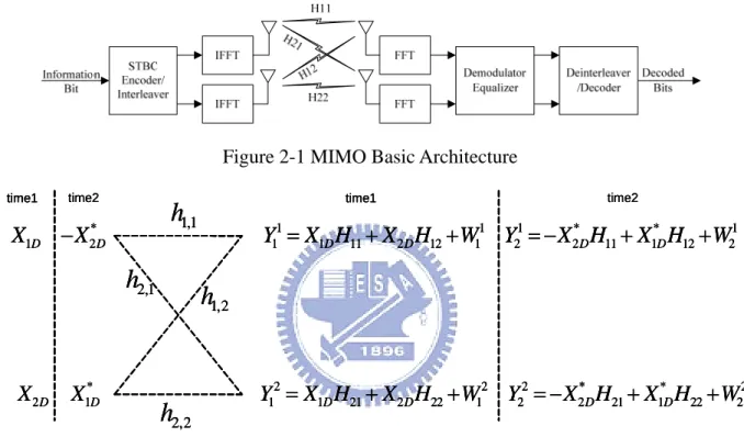
(12) CHAPTER 2 SYSTEM PLATFORM. I. n this chapter, we are going to describe three blocks of wireless communications, transmitter, channel model, and receiver. At first, we introduce the basic of OFDM. and the IEEE 802.11n PHY specification. And then we present the IEEE 802.11n PHY transmitter block diagram. Finally, we propose a universal receiver system model.. 2.1 IEEE 802.11n PHY Specification Orthogonal Frequency Division Multiplexing (OFDM) is a multi-carrier modulation that achieves high data rate and combat multi-path fading in wireless networks. The main concept of OFDM is to divide available channel into several orthogonal sub-channels. All of the sub-channels are transmitted simultaneously, thus achieve a high spectral efficiency. Furthermore, individual data is carried on each sub-carrier, and this is the reason the equalizer can be implemented with low complexity in frequency domain. The MIMO-OFDM system [9] supports BPSK、QPSK、16-QAM、64-QAM four kinds of modulation, FEC supports 1/2、2/3、3/4、5/6 four kinds of coding rate，and it can uses 2x2 or 4x4 antennas to transmit data. Before data transmitted, the data must go through Alamouti STBC（Space Time Block Code）encoding. After that, data go through OFDM modulation, and using IFFT to transfer frequency domain data to time domain signal. In each. 4.

(13) OFDM symbol, each symbol has 64 subcarriers, and 52 of them are data carrier, 4 of them are pilot carrier, others are null carrier. In receiver, first step, it uses FFT to transfer received signal to frequency domain data; second, Equalizer will compensate channel effect then combine two stream data into original by Alamouti Decoder. The MIMO basic architecture is as Figure 2-1 and the Alamouti STBC（ Space Time Block Code ）is as Figure 2-2. Figure 2-1 MIMO Basic Architecture time2. time1. X1D − X 2*D. h2,1. X 2D. X1*D. time1. h1,1. time2. Y11 = X1D H11 + X 2D H12 + W11 Y21 = − X 2*D H11 + X1*D H12 + W21. h1,2. h2,2. Y12 = X1D H21 + X 2D H22 + W12 Y22 = − X 2*D H21 + X1*D H22 + W22. Figure 2-2 Alamouti STBC（Space Time Block Code）. 2.2 System Block Diagram The following two sections comprise of transmitter and receiver are the main parts in our simulation platform. First is the transmitter, and then is the universal receiver.. 2.2.1 Transmitter Figure 2-3 is the transmitter block diagram. After the parameters of data rate and data length are decided, following the blocks one by one will generate the transmitted signals, and 5.

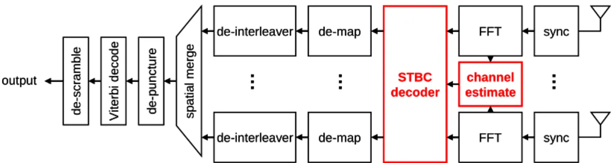
(14) the spatial parse will parse the data streams into several space-time streams which is equal to the transmitter antenna’s number. After STBC encode is the OFDM modulation which will. QAM mapping. spatial streams. Space-time streams. IFFT. Insert GI. analog & RF. …. STBC. …. frequency interleaver. Insert GI. IFFT. …. puncture. QAM mapping. …. spatial parse. frequency interleaver. …. FEC encoder. transform the signal from frequency domain to time domain.. analog & RF. antenna streams. Figure 2-3 MIMO Basic Transmitter. 2.2.2 Receiver Figure 2-4 shows the block diagram of the receiver. After timing synchronization, data will be transformed in to frequency-domain. Then we use the HT preamble to estimate channel frequency response. STBC decoder uses the CFR to decode the space-time code and equalize the data. And this two block also the main part of this thesis. Following is the de-map and de-interleave part. Then all data stream will be merged into single stream by spatial merge block. Finally is the FEC block which includes de-puncturer, Viterbi decoder, and de-scrambler.. spatial merge. de-puncture. de-interleaver. de-map. FFT. STBC decoder. channel estimate. FFT. sync. Figure 2-4 IEEE 802.11n receiver baseband diagram.. 6. sync. …. …. Viterbi decode. de-map. …. output. de-scramble. de-interleaver.

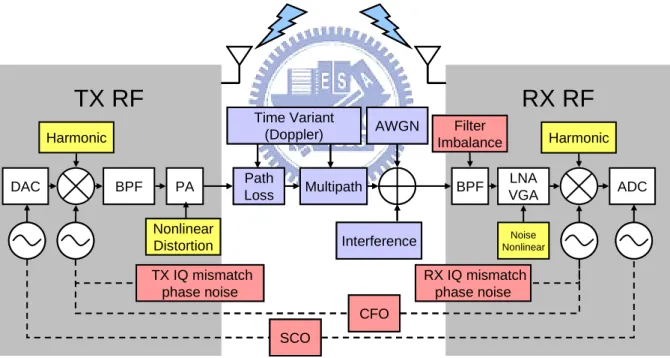
(15) AWGN, time-variant Doppler multipath, carrier frequency offset, phase noise, sampling clock offset and path loss are simulated in the channel, where the AWGN is added, the time-variant Doppler multipath is convoluted, CFO which joint phase noise is multiplied and SCO is convoluted with sinc wave to the Tx signal. The parameter of the AWGN channel is the signal-to-noise ratio (SNR) in dB, and for CFO and SCO is the frequency offset in ppm proportional to the carrier frequency and the symbol sampling frequency respectively. As for the multipath fading channel, the parameters include the channel type, the root-mean-square (rms) delay spread value and the tap numbers. The loop bandwidth and the loop time constant of the low-pass filter in phase-locked loop (PLL) decide the range of phase noise. Figure 2-5 shows the practical and the baseband equivalent channel model.. TX RF. RX RF Time Variant (Doppler). Harmonic. DAC. BPF. PA. Path Loss. AWGN. Multipath. Nonlinear Distortion. Filter Imbalance BPF. LNA VGA Noise Nonlinear. Interference. TX IQ mismatch phase noise. Harmonic. RX IQ mismatch phase noise CFO SCO. Figure 2-5 Baseband equivalent system model. 7. ADC.

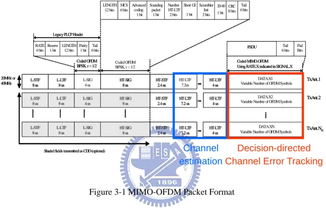
(16) CHAPTER 3 THE PROPOSED DESIGN. I. n this chapter, basic channel estimation and adaptive channel equalization scheme will be proposed. The target OFDM system is the packet-based and burst. synchronization scheme. In a real system, several synchronization issues must be taken care including frame detection (FD), multipath cancellation, and other channel effects. In our design, we will considerate not only our function blocks but also the whole system.. The total compensation scheme contains two partitions. One is the channel estimation using the HT-LTF. The other is adaptive channel equalization for time-varying channel condition. This chapter is the distinguishing feature in the thesis.. 3.1 Channel estimation using interleaving HT-LTF As mention in chapter 2, HT-LTF is tone interleaved across streams, the packet format is as Figure 3-1. The legacy long training OFDM symbol is identical to the 802.11a long training OFDM symbol [9]. And the L-LTF is the same in each antenna. The HT-LTFs are transmitted after the HT-STF. For any PPDU, there must be at least as many HT-LTFs as spatial streams in the HT Data portion of the PPDU. The first HT-LTF consists of two Long Training Symbols (LTS) as in 802.11a/g and a regular guard interval of 0.8 µs, giving a total length of 7.2µs. When present, the second and all subsequent HT-LTFs each consist of a single HT-LTS with a regular guard interval of 0.8 µs, giving a total length of 4µs. And the HT-LTF is tone interleaved across antennas; the 56 tones are partitioned across the antenna array during each. 8.

(17) OFDM symbol. Tone partitioning into sets for 20MHz is shown in Table 3-1. At each OFDM symbol interval, each set of tones maps to one transmit antenna. And over time, all sets get mapped to an antenna. An example of tone interleaving across 4 transmit antennas is shown in Figure 3-2. LENGTH MCS Advanced Sounding packet 12 bits 6 bits coding 1 bit 1 bit. Number Short GI Scrambler 20/40 CRC Tail HT-LTF Init 6 bits 1 bit 8 bits 1 bit 2 bits 2 bits. Legacy PLCP Header RATE Reserve LENGTH Parity Tail 4 bits 1 bit 12 bits 1 bit 6 bits. 20MHz or 40MHz. PSDU. Coded OFDM BPSK, r = 1/2. Coded OFDM BPSK, r = 1/2. Tail 6 bits. Pad Bits. Coded MIMO-OFDM Using RATE.X indicated in SIGNAL.X. L-STF 8 us. L-LTF 8 us. L-SIG 4 us. HT-SIG 8 us. HT-STF 2.4 us. HT-LTF 7.2us. HT-LTF 4 us. DATA.X1 Variable Number of OFDM Symbols. TxAnt.1. L-STF 8 us. L-LTF 8 us. L-SIG 4 us. HT-SIG 8 us. HT-STF 2.4 us. HT-LTF 7.2 us. HT-LTF 4 us. DATA.X2 Variable Number of OFDM Symbols. TxAnt.2. L-STF 8 us. L-LTF 8 us. L-SIG 4 us. HT-SIG 8 us. HT-STF 2.4 us. HT-LTF 7.2 us. HT-LTF 4 us. DATA.XN Variable Number of OFDM Symbols. TxAnt.Ntx. Channel Decision-directed estimation Channel Error Tracking. Shaded fields transmitted as CDD (optional). Figure 3-1 MIMO-OFDM Packet Format. Table 3-1 Tone partitioning of HT-LTF into sets for 20MHz (56 tones) NSTS. Set 0. Set 1. Set 2. 1. [-28:1:-1] [1:1:+28]. 2. [-28:2:-2] [2:2:28]. [-27:2:-1] [1:2:27]. 3. [-28:3:-1] [2:3:26]. [-27:3:-3] [3:3:27]. [-26:3:-2] [1:3:28]. 4. [-28:4:-4] [1:4:25]. [-27:4:-3] [2:4:26]. [-26:4:-2] [3:4:27]. 9. Set 3. [-25:4:-2] [4:4:28].

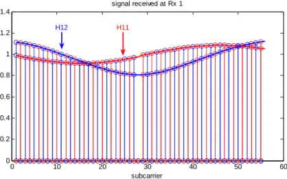
(18) HT-LTF 0. HT-LTF 1. HT-LTF 2. HT-LTF 3. SS 0. Set 0. Set 3. Set 2. Set 1. SS 1. Set 1. Set 0. Set 3. Set 2. SS 2. Set 2. Set 1. Set 0. Set 3. SS 3. Set 3. Set 2. Set 1. Set 0. time. Figure 3-2 HT-LTF tone interleaving across 4 spatial streams. Figure 3-3 shows an example of HT-LTF transmit situation in 2x2 antennas system. time. time. Set0. Set1. Tx1. Rx1. Rx1_1. Rx1_2. Set1. Set0. Tx2. Rx2. Rx2_1. Rx2_2. Figure 3-3 HT-LTF at transmitter and receiver. Figure 3-4 shows the frequency domain of the HT-LTF and the received signal at receiver 1 in 2 time slot. Because the tone interleaved in frequency domain we can estimate the channel frequency response by combining two time slot response at one receiver. Figure 3-5 shows the combining of first antenna and estimated channel. And Figure 3-6 shows the simulation result of estimated channel comparing with the real channel.. Figure 3-4 frequency domain of the HT-LTF and the received signal. 10.

(19) signal received at Rx 1 1.4 H12. 1.2. H11. 1 0.8 0.6 0.4 0.2 0. 0. 10. 20. 30 subcarrier. 40. 50. 60. Figure 3-5 Estimation of H11 and H12 ideal vs estimate channel 1.2. 1.15. 1.1. Amplitude. 1.05. 1. 0.95. 0.9 estimate H11 estimate H12. 0.85. ideal H11 ideal H12. 0.8. 0.75. 0. 10. 20. 30 subcarrier. 40. 50. 60. Figure 3-6 Simulation result of estimated channel. 3.2 Feedback Decision-directed Channel Error Tracking Feedback. DDCET. is. applied. for. high. performance. and. low. complexity.. Computation-save control (CSC) is applied in DDCET to reduce redundant tracking. Channel error tracking can be turned off after several OFDM symbols cause the tracking error is converged to a very small value. The feedback DDCET estimates the CFR error by the de-mapping result of data subcarriers. In data transmission, the system block is shown in 11.

(20) Figure 3-7. The received signal can be shown as. Y11 = X 1D H11 + X 2 D H12 + W11 Y12 = X 1D H 21 + X 2 D H 22 + W12 Y21 = − X 2*D H11 + X 1*D H12 + W21 Y22 = − X 2*D H 21 + X 1*D H 22 + W22 time2. time1. X1D − X 2*D. h2,1. X 2D. X1*D. time2. time1. h1,1. Y11 = X1D H11 + X 2D H12 +W11 Y21 = − X 2*D H11 + X1*D H12 + W21. h1,2 Y12 = X1D H21 + X 2D H22 + W12 Y22 = − X 2*D H21 + X1*D H22 + W22. h2,2. Figure 3-7 STBC transmitter and receiver. Here we assume. H ij = H ijA − ΔH ij. (3.1). where H ij indicates the real channel frequency response between receiver i and transmitter j.. H ijA stands for the adaptive channel frequency response and the estimated CFR error , ΔH ij , and the predicted de-mapping signal, X iD . By STBC decoder , the estimated signal X ie can be written as follows:. (H (H. 2 11 A. 2 11 A. + H12 A + H 21 A + H 22 A. 2. + H12 A + H 21 A + H 22 A. 2. 2. 2. 2. 2. ) X = (Y H 1e. 1 1. * 11 A. ) X = (Y H 2e. 1 1. 12. * 12 A. * 2* + Y21* H12 A + Y12 H 21 A + Y2 H 22 A ) (3.2) * 2* − Y21* H11 A + Y12 H 22 A − Y2 H 21 A ) (3.3).

(21) The estimated signal can be rewrite as. (H. 2 11 A. + H12 A + H 21 A + H 22 A 2. 2. 2. )X =(X 1e. 1D. H11 + X 2 D H12 + W11 ) H11* A. + ( − X 2*D H11 + X 1*D H12 + W21 ) H12 A *. (3.4). * + ( X 1D H 21 + X 2 D H 22 + W12 ) H 21 A. + ( − X 2*D H 21 + X 1*D H 22 + W22 ) H 22 A *. (H. 2 11 A. + H12 A + H 21 A + H 22 A 2. 2. 2. )X =(X 2e. 1D. H11 + X 2 D H12 + W11 ) H12* A. − ( − X 2*D H11 + X 1*D H12 + W21 ) H11 A *. (3.5). * + ( X 1D H 21 + X 2 D H 22 + W12 ) H 22 A. − ( − X 2*D H 21 + X 1*D H 22 + W22 ) H 21 A *. If we assume only H11 has estimated CFR error, then the equations becomes:. (H. 2 11 A. + H12 A + H 21 A + H 22 A 2. 2. 2. )X =(X 1e. 1D. ( H11 A − ΔH11 ) + X 2 D H12 A + W11 ) H11* A. + ( − X 2*D ( H11 A − ΔH11 ) + X 1*D H12 A + W21 ) H12 A *. * + ( X 1D H 21 A + X 2 D H 22 A + W12 ) H 21 A. (3.6). + ( − X 2*D H 21 A + X 1*D H 22 A + W22 ) H 22 A *. (H. 2 11 A. + H12 A + H 21 A + H 22 A 2. 2. 2. )X =(X 2e. 1D. ( H11 A − ΔH11 ) + X 2 D H12 A + W11 ) H12* A. − ( − X 2*D ( H11 A − ΔH11 ) + X 1*D H12 A + W21 ) H11 A *. * + ( X 1D H 21 A + X 2 D H 22 A + W12 ) H 22 A. − ( − X 2*D H 21 A + X 1*D H 22 A + W22 ) H 21 A *. By elimination the same item in the equation, we get:. 13. (3.7).

(22) (H. 2 11 A. + H12 A + H 21 A + H 22 A 2. 2. 2. )X. 1e. = X 1D H11 A H11* A − X 1D ΔH11 H11* A + X 2 D H12 A H11* A − X 2 D H11* A H12 A + X 2 D ΔH11* H12 A + X 1D H12* A H12 A * * + X 1D H 21 A H 21 A + X 2 D H 22 A H 21 A * * − X 2 D H 21 A H 22 A + X 1D H 22 A H 22 A * 2* +W11 H11* A + W21* H12 A + W12 H 21 A + W2 H 22 A. (. = H11 A + H12 A + H 21 A + H 22 A 2. 2. 2. 2. )X. 1D. − X 1D ΔH11 H11* A + X 2 D ΔH11* H12 A * 2* +W11 H11* A + W21* H12 A + W12 H 21 A + W2 H 22 A. (3.8). (H. 2 11 A. + H12 A + H 21 A + H 22 A 2. 2. 2. )X. 2e. = X 1D H11 A H1*2 A − X 1D ΔH11 H12* A + X 2 D H12 A H12* A + X 2 D H11* A H11 A − X 2 D ΔH11* H11 A − X 1D H12* A H11 A * * + X 1D H 21 A H 22 A + X 2 D H 22 A H 22 A * * + X 2 D H 21 A H 21 A − X 1D H 22 A H 21 A * 2* +W11 H12* A − W21* H11 A + W12 H 22 A − W2 H 21 A. (. = H11 A + H12 A + H 21 A + H 22 A 2. 2. 2. 2. )X. 2D. − X 1D ΔH11 H12* A − X 2 D ΔH11* H11 A * 2* +W11 H12* A − W21* H11 A + W12 H 22 A − W2 H 21 A. (3.9) now we have. (. ). (. ). (. ). (. ). ⎧ H 2+ H 2+ H 2+ H 2 X = H 2+ H 2+ H 2+ H 2 X 12 A 21 A 22 A 1e 11 A 12 A 21 A 22 A 1D ⎪ 11 A ⎪ − X 1D ΔH11 H11* A + X 2 D ΔH11* H12 A ⎪ * 2* ⎪⎪ +W11 H11* A + W21* H12 A + W12 H 21 A + W2 H 22 A (3.10) ⎨ 2 2 2 2 2 2 2 2 ⎪ H11 A + H12 A + H 21 A + H 22 A X 2 e = H11 A + H12 A + H 21 A + H 22 A X 2 D ⎪ ⎪ − X 1D ΔH11 H12* A − X 2 D ΔH11* H11 A ⎪ * 2* +W11 H1*2 A − W21* H11 A + W12 H 22 ⎪⎩ A − W2 H 21 A. By combining X 1D and X 1e , we get:. 14.

(23) ( (. ⎧ X ΔH H * − X ΔH * H = H 2 + H 2 + H 2 + H 2 2D 11 12 A 11 A 12 A 21 A 22 A ⎪ 1D 11 11 A ⎨ 2 2 2 2 ⎪ X 1D ΔH11 H12* A + X 2 D ΔH11* H11 A = H11 A + H12 A + H 21 A + H 22 A ⎩. )( X )( X. 1D. − X 1e ) + W1 (3.11). 2 D − X 2 e ) + W2. Then multiply the first equation by H11A , and the second equation by H12 A :. ⎧ H ( X ΔH H * − X ΔH * H ) = H 2D 11 12 A 11 A ⎪ 11 A 1D 11 11 A ⎨ ⎪ H12 A ( X 1D ΔH11 H12* A + X 2 D ΔH11* H11 A ) = H12 A ⎩. (( H (( H. 2. 11 A 2 11 A. + H12 A + H 21 A + H 22 A. 2. + H12 A + H 21 A + H 22 A. 2. 2. 2. 2. 2. )( X )( X. − X 1e ) + W1. 1D. ). − X 2 e ) + W2. 2D. ). (3.12). ⎧ X ΔH H * H − X ΔH * H H = H 2D 11 12 A 11 A 11 A ⎪ 1D 11 11 A 11 A ⎨ ⎪ X 1D ΔH11 H12* A H12 A + X 2 D ΔH11* H11 A H12 A = H12 A ⎩. (( H (( H. 2. 11 A 2 11 A. + H12 A + H 21 A + H 22 A. 2. + H12 A + H 21 A + H 22 A. 2. 2. 2. 2. )( X )( X. 1D. 2. 2D. − X 1e ) + W1. − X 2 e ) + W2. (3.13) By adding two equations, we get the following. (H. 2 11 A. + H12 A. 2. )X. 1D. ΔH11 = H11 A + H12 A. (( H (( H. 2 11 A 2 11 A. + H12 A + H 21 A + H 22 A. 2. + H12 A + H 21 A + H 22 A. 2. 2. 2. 2. 2. )( X )( X. ) ) +W ). 1D. − X 1e ) + W1. 2D. − X 2e. 2. (3.14) and we can find ΔH11 by:. (( H + H (( H = H11 A. ΔH11. 12 A. 2. 11 A. + H12 A + H 21 A + H 22 A 2. 2 11 A. 2. 2. 1D. + H12 A + H 21 A + H 22 A 2. (H. 2. 2 11 A. + H12 A. 2. )X. )( X − X ) +W ) )( X − X ) +W ) 1e. 1. 2. 2D. 2e. 2. (3.15). 1D. By repeating the procedure above with different assumption on H ij , we can obtain 4 estimated. 15. ). ).

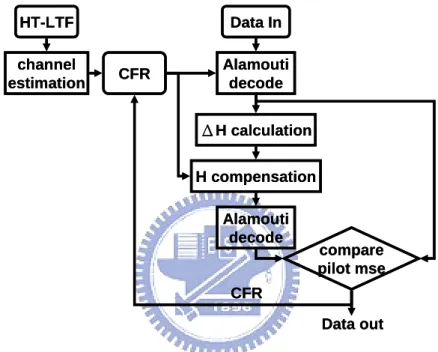
(24) CFR error as follows:. (( H + H (( H = H11 A. ΔH11. 12 A. 2. ΔH 21 =. H 21 A ΔH 22 =. 2. + H12 A. )X. 2. 2 11 A. 2. 2. + H12 A. 2. )X. 2. (H. 21 A. + H 22 A. 2. 2. 2 11 A. 2. )X. 2. (H. 2. 2 21 A. + H 22 A. 2. 1e. 1. 2. 2D. 2e. 2. )X. )( X − X ) +W ) )( X − X ) +W ) 1D. 1e. 1. 2. 2D. 2e. 2. 1D 2. )( X − X ) +W ) )( X − X ) +W ) 1D. + H12 A + H 21 A + H 22 A 2. 2. )( X − X ) +W ) )( X − X ) +W ). 2. 2. 2e. 2D. + H12 A + H 21 A + H 22 A. 2. 2D. + H12 A + H 21 A + H 22 A 2. 1. 2. 1D. 2. 11 A. 1e. 1D. + H12 A + H 21 A + H 22 A. 2. 11 A. + H 22 A. 11 A. 2. + H12 A + H 21 A + H 22 A. 2. (( H (( H. 2. )( X − X ) +W ) )( X − X ) +W ) 1D. 2. 2. (H. 11 A. + H 22 A. 2. 2. 11 A. 2. + H12 A + H 21 A + H 22 A. + H12 A + H 21 A + H 22 A. 2. (( H (( H. 2. (H. 11 A. 12 A. H 21 A. 2. 11 A. (( H + H (( H = H11 A. ΔH12. + H12 A + H 21 A + H 22 A. 2. 11 A. 1e. 1. 2. 2D. 2e. 2. (3.16). 2D. After that, we compare the equalized pilots with the known one and compute the mean-square error as the error function. Then we judge if this corrected CFR is suitable. If the MSE of the compensated pilots, MSEcomp, is greater than the MSE of the original pilots before compensated, MSEori, we discard this CFR. Otherwise, the old CFR will be replaced by the suitable one. The algorithm of this feedback loop is. MSEori =. 1 M. MSEcomp =. M. ∑ P (k ) − P (k ) k =1. 1 M. e. M. ∑P k =1. 2. (3.17). D. improve. (k ) − PD (k ). 2. (3.18). ⎧⎪ H A (k ) − μ ⋅ ΔH l −1 (k ), if MSEcomp > MSEori H A ,l ( k ) ≈ ⎨ , if MSEcomp ≤ MSEori ⎪⎩ H A (k ). 16. (3.19).

(25) where M is the number of pilots and μ is the step size of the adaptive tracking loop. Under the feedback tracking algorithm which adjusts the CFR directly instead of compensating the data subcarriers only, we can get more accurate data subcarriers to make more precise estimations of CFR error.. Figure 3-8 is the flow chart of the proposed algorithm.. HT-LTF channel estimation. Data In CFR. Alamouti decode ΔH calculation H compensation Alamouti decode. compare pilot mse. CFR Data out. Figure 3-8 Algorithm flow chart. 17.

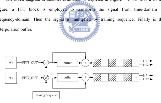
(26) CHAPTER 4 HARDWARE ARCHITECTURE AND PERFORMANCE ANALYSIS. T. he whole architecture of the proposed adaptive equalization can be divided into three parts, the channel estimation, the Space-Time Block code decoder, and. adaptive channel equalizer.. The block diagram of channel estimation is depicted in Figure 4-1. As shown in the figure, a FFT block is employed to transform the signal from time-domain to frequency-domain. Then the signal is multiplied by training sequence. Finally is the interpolation buffer.. Figure 4-1 Channel estimation architecture. Figure 4-2 shows the architecture of Alamouti Space-time Block code decoder. As shown in Figure 4-3, signal will be decoded two times with the original CFR and adaptive CFR, then decided by pilot MSE comparator to choose the better one. 18.

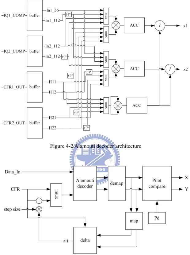
(27) Figure 4-2 Alamouti decoder architecture. Figure 4-3 Adaptive channel equalizer. 19.

(28) To evaluate the proposed algorithm, a typical MIMO-OFDM system based on IEEE 802.11n Wireless LANs, TGn Sync Proposal Technical Specification, is used as a reference-design platform. The parameters used in the simulation platform are “The length of OFDM symbol is 64 and cyclic prefix is 16”. A satisfactory accuracy can usually be reached if enough data samples are used to calculate the estimate from the long training symbols. As a result, the proposed method uses high throughput long training field symbols and legacy long training field symbols to measure the frequency dependent I/Q-M.. The simulation result below is based on following conditions: z. 2x2 MIMO-OFDM systems in 20MHhz.. z. PSDU is 1024. bytes. z. MCS is 14 (modulation is 64QAM, coding rate is 3/4 ). z. Decoder using soft Viterbi decoder. Multipath Model: TGn-E and the relative rms delay and Tap number will be shown in Table 4-1. 20.

(29) Table 4-1 TGn Multipath Specifications. Mode. rms delay spread. Tap numbers. A. 0 ns. 1. B. 15 ns. 2. C. 30 ns. 5. D. 50 ns. 8. E. 100 ns. 15. F. 150 ns. 22. Figure 4-4 and Figure 4-5 show example of channel impulse response and channel frequency response in 60km/hr situation.. Figure 4-4 Channel impulse response in 60 km/hr. 21.

(30) Figure 4-5 Channel frequency response in 60 km/hr. Figure 4-6 shows that the CFR mean-square-error between adaptive channel and the real channel is decrease, which means the adaptive channel is more and more close to the real channel. Figure 4-7 shows that the data MSE between decode data and real data is also decrease. CFR MSE 0.038. 0.036. 0.034. 0.032. 0.03. 0.028. 0.026. 0.024. 0.022. 0.02. 0. 5. 10. 15 20 OFDM symbol. 25. Figure 4-6 CFR MSE. 22. 30. 35.

(31) -3. 8. data MSE. x 10. 7.5. 7. 6.5. 6. 5.5. 5. 4.5. 4. 3.5. 3. 0. 5. 10. 15 20 OFDM Symbol. 25. 30. 35. Figure 4-7 Data MSE. Following figure will show the whole system performance ( BER and PER ) improved by the proposed algorithms. In Figure 4-8 and Figure 4-9 , the multipath condition is time-varying TGnD, the proposed algorithms can improve the system performance greatly when the channel is time-varying. BER vs SNR. -1. 10. no improve improve. -2. 10. -3. 10. -4. 10. 20. 22. 24. 26. 28. 30. 32. 34. Figure 4-8 Bit Error Rate. 23. 36. 38. 40.

(32) PER vs SNR. 0. 10. no improve improve. 20. 22. 24. 26. 28. 30. 32. 34. 36. 38. 40. Figure 4-9 Packet Error Rate BER vs SNR. error rate. 10. 10. -1. -2. 10km/hr no improve 10km/hr no improve self 60km/hr no improve 120km/hr no improve 180km/hr no improve 60km/hr step size=0.05 120km/hr step size=0.05 180km/hr step size=0.05 -3 60km/hr 10 step size=0.1 120km/hr step size=0.1 60km/hr step size=0.025 120km/hr 20 step size=0.02522 10km/hr step size=0.025 10km/hr step size=0.025 self. 24. 26. 28. 30. 32. SNR. Figure 4-10 BER with different velocity and different step-size. 24. 34.

(33) PER vs SNR 0. error rate. 10. 10km/hr no improve 10km/hr no improve self 60km/hr no improve 120km/hr no improve -1 180km/hr no improve 10 60km/hr step size=0.05 120km/hr step size=0.05 180km/hr step size=0.05 60km/hr step size=0.1 120km/hr step size=0.1 60km/hr step size=0.025 120km/hr step size=0.025 10km/hr step size=0.025 20 22 10km/hr step size=0.025 self. 24. 26. 28. 30. 32. 34. SNR. Figure 4-11 PER with different velocity and different step-size. From the simulation result we can see that the performance degrade seriously with only one shot channel estimation in time-varying channel situation. This thesis proposes a novel scheme for channel equalization in OFDM receivers. The proposed algorithm can use de-mapping results and pilots to adjusting estimate channel frequency response in time-varying channel environments. From simulation results, the average estimation error of the proposed algorithm is small enough for little system performance loss under different multipath channel. And the convergence speed is much faster at the same time. Besides, the proposed method is suitable for implementation issue. 25.

(34) CHAPTER 5 CONCLUSION AND FUTURE WORK. T. his thesis has proposed a novel one-shot algorithm to estimate the channel in MIMO-OFDM receivers. The proposed algorithm can use High-Throughput long. training symbols to estimate channel in time-variant Doppler multipath environments. Besides, the proposed adaptive channel equalizer can modify the channel frequency response to approach the real channel frequency response. From simulation results, the proposed algorithm can meet many system requirements to prevent obvious performance loss under time-varying channel condition. Table 5-1 shows the comparison of state-of-the-art equalizer.. Table 5-1 Comparison of state-of-the-art adaptive equalization. Operating Domain. JSAC.1999[10]. ISPACS.2005 [11]. [12]. This work. Time. Frequency. Frequency. Frequency. Decision-directed. Decision-directed. Decision-directed. Pilot. Pilot. Pilot. Optimum Training Method Sequence Property Utilization. N/A. Standard compatible. N/A. IEEE 802.11n. IEEE 802.11n IEEE 802.11a. TGn sync proposal Modulation. 4-PSK. 16-QAM. Two-ray,TU,HT delay. ETSI Multipath channel. Channel Condition. Space-Time code. TGn sync proposal 64-QAM. 64-QAM IEEE rms 50 , 8 taps. IEEE rms 50 , 13 taps with fd = 40 Hz. with Jake’s model. 16-State. STBC. Requires high Note. time-varying model N/A. STBC. large improvement in. Deal well with random. singular channel. changed channel model. Not fully support spec computational complexity. 26.

(35) References [1] S. Alamouti, “A simple transmit diversity technique for wireless communications,” IEEE J. Select. Areas Commun., pp. 1451–1458, Oct. 1998. [2] IEEE 802.11g, IEEE Standard for Wireless LAN Medium Access Control and Physical Layer Specifications, June 2003. [3] TGn Sync, TGn sync proposal technical specification, IEEE 802.11 11-04-0889-07-000n-tgnsync-proposal-technical-specification , July 2005 [4] Zheng Yuanjin, "A novel channel estimation and tracking method for wireless OFDM systems based on pilots and Kalman filtering", in IEEE Transactions on Consumer Electronics, vol 49, pp 275-283, May 2003. [5] Schafhuber, D.; Matz, G.; Hlawatsch, F.,"Kalman tracking of time-varying channels in wireless MIMO-OFDM systems", in Proc. of Conference Record of the Thirty-Seventh Asilomar Conference, vol 2, pp 1261 - 1265, Nov. 2003 [6] Grunheid, R.; Rohling, H.; Jianjun Ran; Bolinth, E.; Kern, R., "Robust channel estimation in wireless LANs for mobile environments", in Proc. on Vehicular Technology Conference 2002. ,vol 3, pp 1545 - 1549, Sept. 2002. [7] Dowler, A.; Nix, A.; McGeehan, J., "Data-Derived Iterative channel Estimation with Channel tracking for a mobile fourth generation wide area OFDM system", in Proc. of GLOBECOM '03. vol 2, pp 804 - 808, Dec. 2003 [8] Ran, J.; Grunheid, R.; Rohling, H.; Bolinth, E.; Kern, R," Decision-directed Channel Estimation Method for OFDM systems with high velocities", in Proc. of Vehicular Technology Conference 2003. vol 4, pp 2358 - 2361, April 2003. [9] 11-04-0889-04-000n-tgnsync-proposal-technical-specification, IEEE, 2005. 27.

(36) [10] Ye Li; Seshadri, N.; Ariyavisitakul, S.,”Channel estimation for OFDM systems with transmitter diversity in mobile wireless channels”, IEEE JOURNAL ON SELECTED AREAS IN COMMUNICATIONS,1999 [11] Ying Chen, Dhammika Jayalath, Thushara, Abhayapala,”LOW COMPLEXITY DECISION DIRECTED CHANNEL TRACKING FOR MIMO WLAN SYSTEM”, International Symposium on Intelligent Signal Processing and Communication Systems,2005 [12] Ming-Yeh Wu, “Design of Pilot-based Adaptive Equalization for Wireless OFDM Baseband Applications”, nctu thesis,2004. 28.

(37) Vita Ta-Yang Juan, male, was born in Chang-Hua County, Taiwan, R.O.C., on May 23, 1981.. He received the B.S. degree in Computer Science and Information Engineering from National Chiao Tung University, Hsinchu, Taiwan, in 2004 and make efforts in master degree at Nation Chiao Tung University from September 2004. His main interests lay in the field of wireless communications and signal processing. His research has been focused on physical layer issues related to channel estimation and equalizer in OFDM systems.. 29.

(38)