生產者與中間商利潤模式有量測誤差下規格之最適設計 - 政大學術集成
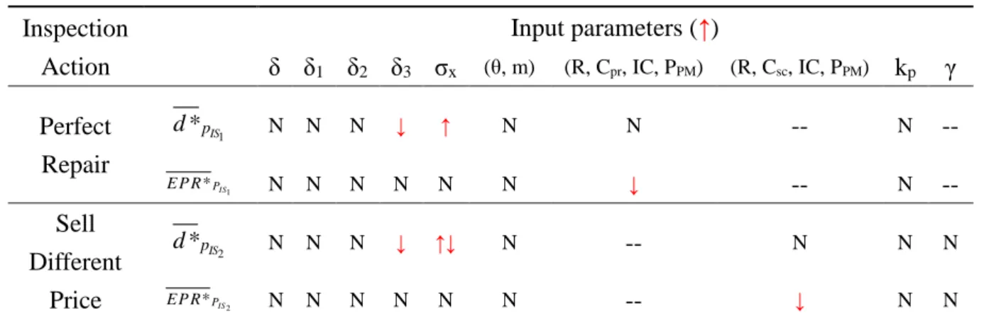
163
0
0
全文
(2) 謝辭. 兩年的研究生生涯即將進入尾聲,兩年來不僅於學業上學習到許多的知識,也學習到面對 挑戰,克服挫折及自我調適的能力與態度。能夠順利完成這篇論文,我要感謝這些日子以來幫 助及鼓勵我的人。 首先最要感謝的是我的指導老師 楊素芬教授,感謝楊老師這兩年來的辛苦的教導及栽培, 不但讓我學習到許多的品管上的專業知識,也教導了我許多為人處事的道理 接著要感謝 唐正教授與 曾勝滄教授於百忙之中撥冗前來擔任口試委員,並對我的論文提 出了許多可以精進之處,讓我的論文能夠更臻完善,也要感謝兩位教授於口試之後給予的勉勵 及祝福。. 治 政 大 感謝碩士班兩年來陪伴及幫助我的同學們,因為有你們陪伴與幫助,讓我在碩士生涯過得 立. 十分充實與精彩,並讓我有勇氣面對諸多的問題。. ‧ 國. 學. 最後一定要感謝的是我的家人,感謝你們對我的鼓勵以及支持,讓我在遭遇挫折的時候能. sit. y. Nat. 國家有所貢獻。. ‧. 夠一一克服,並能無後顧之憂的專注於學業上,在未來我也將更加努力,希望能對我的家庭及. io. al. er. 本研究承蒙以下單位補助,謹此致謝︰. n. 1. 行政院國家科學委員會,專題研究計畫編號 NSC 100-2118-M-004-003-MY2。 2.. Ch 政治大學商學院頂尖大學研究計畫。. engchi. i Un. v. 3. 政治大學研究團隊計畫。 本項結果使用國家高速網路與計算中心之計算資源,特此感謝。. 林裕景 謹致 中華民國一百零二年六月.
(3) Abstract Measurement error is an important issue in quality control, so in this study a producer instrument with measurement error is considered. When its instrument contains measurement error, we assume that a producer takes either complete inspection or on-line process control to maintain products quality. We then compare their respective profits to choose a better quality control policy. Also in the complete inspection plan we consider perfect repair and selling at a lower price are two actions for a producer to deal with nonconforming items. Under the maximizing profit model, we determine the optimal specification limits for the producer, and then compare the profit of these two actions to determine. 政 治 大 In this article we also consider the act of a middleman. We assume that the specification limits of 立. which action is better for producer to take.. the middleman and producer are the same and the product that middleman bought may come from. ‧ 國. 學. perfect repair action or selling at a lower price action. When maximizing the middleman’s profit, we. ‧. determine the specification limits, buying and selling price of middleman, and we also compare the. sit. y. Nat. profit from these two actions to find out which action is better for the middleman.. io. er. In our analysis, we found that when process has a small production per unit time, a high repair. al. iv n C by producer; otherwise the producer should take h ecomplete i U And to have a larger profit, n g c hinspection. n. cost, a high cost of nonconforming item, and a high sell price, then process control should be preferred. middleman should buy products from producer who took the action of perfect repair when middleman’s instrument contains measurement error or middleman’s instrument contains no measurement error but producer’s instrument contains a small measurement error.. Keywords: Measurement error; Perfect repair action; Sell low price action; Middleman. I.
(4) CONTENT CHAPTER 1. INTRODUCTION .......................................................................................................... 1 1.1 Literature Review and Study Motivation ........................................................................................... 1 1.2 Research Method ................................................................................................................................ 4 CHAPTER 2. MAXIMIZE PRODUCER PROFIT UNDER INSTRUMENT WITH MEASUREMENT ERROR .......................................................................................... 6 2.1 Notations ............................................................................................................................................. 7 2.2 Assumptions for Quality Variables ..................................................................................................... 7 2.3 Complete Inspection and Adopting Two Actions for Observed Nonconforming Items ..................... 9 2.3.1 Perfect repair for observed nonconforming items .................................................................... 9 2.3.2 Taking sell low price action for observed nonconforming items............................................ 23 2.4 Process Control Using EWMAYP − EWMAlnSY2 Chart .......................................................................... 40. 政 治 大 P. 2.4.1 Parameters notation ................................................................................................................ 40. 立. 2.4.2 Establish EWMAYP − EWMAlnSY2 chart. ......................................................................................... 41 P. ‧ 國. 學. ‧. 2.4.3 Derivation of the profit model per unit time. .......................................................................... 45 2.4.4 Determine the optimal design parameters and data analyses. ................................................ 47 2.5 Comparing the Expected Profit Per Unit Time for Complete Inspection Plan and Process Control. ......................................................................................................................................................... 55. y. Nat. sit. n. al. er. io. CHAPTER 3. DERIVE AND COMPARE THE MIDDLEMAN PROFITS PER ITEM UNDER PRODUCER TAKING TWO ACTIONS .................................................................. 62 3.1 Notations ........................................................................................................................................... 62 3.2 Maximize the Profit Model to Determine the Optimal Specification Limits for Middleman under Producer Adopts Perfect Repair Action .......................................................................................... 63 3.2.1 Derivation of the profit model for middleman. ...................................................................... 63 3.3 Maximize the Profit Model to Determine the Optimal Specification Limits for Middleman under Producer Adopts Sell Low Price Action.......................................................................................... 83. Ch. engchi. i Un. v. 3.3.1 Derivation of the profit model for middleman ....................................................................... 83 3.3.2 Determine the optimal specification limits, middleman buying and selling price with Data analyses. ................................................................................................................................. 91 3.4 Compare Expected Profit per item for Middleman under Producer Take Different Actions. ........ 102 3.4.1 Compare profits of middleman for middleman instrument without measurement error under producer’s two actions ......................................................................................................... 102 3.4.2 Comparing the four cases expected profit of middleman for middleman instrument with measurement error. .............................................................................................................. 105 CHAPTER 4. DERIVE THE MIDDLEMAN PROFIT MODEL WITH CONSIDERING ORDER QUANTITY UNDER PRODUCER TAKING TWO ACTIONS ........... 110 4.1 Notations ......................................................................................................................................... 110 II.
(5) 4.2 Describe the Sell Price and Order Quantity Relationship among Producer, Middleman and Customer ........................................................................................................................................ 110 4.3 Maximize the Profit Model to Determine the Optimal Specification Limits, Order Quantity, Buying and Selling Price for Middleman under Producer Adopting Perfect Repair Action. ..................... 111 4.3.1 Derivation of the profit model with order quantity for middleman. ..................................... 111 4.3.2 Determine the optimal specification limits, middleman order quantity, buying and selling price for middleman with the data analyses. ....................................................................... 115 4.3.3 Comparing the middleman ordered quantity and middleman profit for middleman instrument without and with measurement error under producer taking perfect repair action.............. 118 4.4 Maximize the Profit Model to Determine the Optimal Specification Limits, Order Quantity, Buying and Selling Price for Middleman under Producer Adopting Sell Low Price Action. .................... 121 4.4.1 Derivation of the profit model with order quantity for middleman. ..................................... 121 4.4.2 Determine the optimal specification limits, middleman order quantity, buying and selling price for middleman with the data analyses. ....................................................................... 129 4.4.3 Comparing the middleman ordered quantity and middleman profit for middleman instrument with and without measurement error under producer taking sell low price action. ............ 132 4.5 Compare Expected Profit per Week for Middleman under Producer Take Different Actions. ...... 135 4.5.1 Comparing ordered quantity and expected profit of the middleman for middleman instrument without measurement error. ................................................................................................. 135 4.5.2 Comparing ordered quantity and expected profit of the middleman for middleman instrument with measurement error. ...................................................................................................... 138. 立. 政 治 大. ‧. ‧ 國. 學. n. al. er. io. sit. y. Nat. CHAPTER 5. SUMMARY AND FUTURE STUDY ....................................................................... 143 REFERENCES ................................................................................................................................... 145 APPENDIXES ..................................................................................................................................... 147 Appendix A. Derive the Distribution of X PI | YPI = y ........................................................................... 147. Ch. i Un. v. Appendix B. Calculate the Average Run Length .................................................................................. 148. engchi. III.
(6) LIST OF TABLES Table 1.1 The framework of this article .................................................................................................... 5 Table 2.1 Numeric example for finding true quality distribution (XM) of products received by middleman ............................................................................................................................. 15 Table 2.2 The number of simulate data in each interval and expected frequency .................................. 16 Table 2.3 Three Levels of Each Parameters ........................................................................................... 17 13 Table 2.4 The 27 combinations of these parameters by using an orthogonal array table L27 (3 ) . ....... 18. Table 2.6 Table Response table of d*P .................................................................................................... 20 Table 2.7 Response table of EPR* PIS1 ..................................................................................................... 21. 政 治 大. Table 2.8 The optimal solutions of the 18 combinations of parameters under different η value ........... 22 Table 2.9 Three Levels of Each Parameters ........................................................................................... 26 Table 2.10 The 27 combinations of these parameters by using an orthogonal array table L27 (313 ) . .......... 27. 立. ‧ 國. 學. Table 2.11 Optimal solutions of the 27 combinations parameters. ......................................................... 28 Table 2.12 Response table of d*P ........................................................................................................... 29 EPR*PIS2. ‧. Table 2.13 Response table of. ....................................................................................................... 30. y. Nat. Table 2.14 Summary table for sensitivity analyses of perfect repair and sell different price ................. 31. er. io. sit. Table 2.15 The 27 parameters combinations with Dd PIS and DEPRPIS ..................................................... 32 Table 2.16 Yield of true quality and observed quality for two actions that producer took ..................... 33. n. al. iv. Ch Table 2.17 Response table of DdPIS ......................................................................................................... 34 Un engchi. Table 2.18 Response table of DEPRPIS ...................................................................................................... 35 Table 2.19 Three Levels of Each Parameters ......................................................................................... 47 Table 2.20 The 27 combinations of these parameters by using an orthogonal array table L27 (313 ) . ........ 48 Table 2.21 The optimal solutions of the 27 combination parameters ..................................................... 49 Table 2.22 Response table of n * ........................................................................................................... 50 Table 2.23 Response table of h * ........................................................................................................... 51 Table 2.24 Response table of ARL1 * ...................................................................................................... 52 Table 2.25 Response table of EPR * SPC .................................................................................................. 53 Table 2.27 Response table of D * I S − S P C ............................................................................................... 55 Table 2.28 Response table of D * I S − S P C ............................................................................................... 56 Table 2.29 Summary table of sensitivity analyses for D * I S − S P C and D * I S − S P C ............................... 57 1. 2. 1. 2. Table 2.30 Parameters range for producer conducting complete inspection plan under different η combination values .............................................................................................................. 61 IV.
(7) Table 3.1 Three Levels of each Parameter .............................................................................................. 70 Table 3.2 The 27 combinations of these parameters by using an orthogonal array table L27 (313 ) . ............ 71 EPR*MR−WO > EPR*MR−W .2 > EPR*MR−W .1 > EPR*MR−W .4 > EPR*MR−W .3 . .................................................... 72. Table 3.3 The optimal solutions of 27 combinations of parameters when PPMLB=50, PMCU=90, under producer taking perfect repair action. .................................................................................... 73 * * * * Table 3.4 The EPRR−D1 , EPRR − D2 , EPRR − D3 and EPRR − D4 values with different parameters. combination under producer taking perfect repair action ...................................................... 76 Table 3.5 Response table of EPR * R − D , E P R * R − D , EPR * R − D and E P R * R − D ..................................... 77 Table 3.6 Summary table of sensitivity analyses for EPR * R − D , E P R * R − D , EPR * R − D and E P R * R − D ............................................................................................................................................... 79 1. 2. 3. 4. 1. 2. 3. 4. * * * * * * Table 3.7 The EPRR.W − D1 , EPRR.W −D2 , EPRR.W −D3 , EPRR.W −D4 , EPRR.W −D5 and EPRR.W −D6 values. 政 治 大 , ,. under different combinations of parameters for producer taking perfect repair action ......... 81. 立. Table 3.8 Response table of EPR * R .W − D , E P R * R .W − D EPR * R .W − D E P R * R .W − D , EPR * R .W − D and EPR * R .W − D ......................................................................................................................... 82 Table 3.9 Three Levels of Each Parameters ........................................................................................... 91 Table 3.10 The 27 combinations of these parameters used in an orthogonal array table L 27 (313 ) . ........ 92 1. 6. 2. 3. 4. 5. ‧ 國. 學. EPR * S − D 2. ,. EPR * S − D3. , and. EPR * S − D 4. y. ,. values with different combinations of. sit. EPR * S − D1. Nat. Table 3.12 The. ‧. Table 3.11 The optimal solutions of 27 combinations of parameters when PPMLB=50, PMCU=90, under producer taking selling low price action.............................................................................. 93. n. al. er. io. parameters under producer taking perfect repair action. ....................................................... 96. v ni. Table 3.13 Response table of EPR * S − D , EPR * S − D , EPR * S − D , and EPR * S − D for each parameters ...... 97 Table 3.14 Sensitivity analyses summary table of EPR * S − D , EPR * S − D , EPR * S − D , and EPR * S − D ....... 98 Table 3.16 Response table of EPR * S .W − D , EPR * S .W − D , EPR * S .W − D , EPR * S .W − D , EPR * S .W − D , and EPR * S .W − D ........................................................................................................................... 101 1. 1. 2. Ch. 3. engchi U 1. 2. 3. 4. 2. 3. 4. 4. 5. 6. * Table 3.17 The EPRR−S.DO values for different combinations of parameters ........................................ 103. Table 3.18 Response table of. E P R * R − S .D O. ........................................................................................... 104. * * * * Table 3.19 The EPRR−S.D1 , EPRR−S.D2 , EPRR−S.D3 and EPRR−S.D4 values for different combinations of. parameters .......................................................................................................................... 106 Table 3.20 Response table of EPR * R − S .D , EPR * R − S .D , EPR * R − S .D and EPR * R − S .D ............................ 107 Table 4.1 Three Levels of Parameters Levels ....................................................................................... 115 Table 4.2 The 27 combinations of these parameters by using an orthogonal array table L 27 (313 ) . ...... 116 1. 2. 3. 4. Table 4.3 The optimal solutions of 27 combinations of parameters when PPMLB=50, PMCU=90, a=0, and b=300 under producer taking perfect repair action. ............................................................ 117 Table 4.4 The Q*M QR − D and EPR*MQR−D values for different combinations of parameters under producer V.
(8) taking perfect repair action .................................................................................................. 119 Table 4.5 Response tables of Q*MQR−D and EPR*MQR−D ........................................................................ 120 Table 4.6 Three Levels of Each Parameters ......................................................................................... 129 Table 4.7 The 27 combinations of these parameters by using an orthogonal array table L27 (313 ) . .......... 130 Table 4.8 The optimal solutions of 27 combinations of parameters. .................................................... 131 Table 4.9 The Q*M QS − D and EPR*MQS−D values with different combinations of parameters under producer taking sell low price action ................................................................................... 133 Table 4.10 Response table of Q*MPQS −D and E P R * M. QS −D. ......................................................................... 134. * * Table 4.11 The QQR − QS .DWO and EPRQR−QS.DWO values for different combinations of parameters ...... 136. Table 4.12 Response table of. EPR * Q R − Q S .DW O. ........................................................................................ 137. 政 治 大. * * Table 4.13 QQR−QS.DW and EPRQR −QS .DW values for different combinations of parameters .................. 139. 立. .............................................................. 140. ‧. ‧ 國. E P R * Q R − Q S .DW. 學. Table 4.14 Response table of Q*QR−QS.DW and. n. er. io. sit. y. Nat. al. Ch. engchi. VI. i Un. v.
(9) LIST OF FIGURES Figure 2.1 Producer specification based on YP, nonconforming item may perfect repaired with repair cost Cpr. .................................................................................................................................... 9 Figure 2.2 Quadratic loss function based on XP ..................................................................................... 10 Figure 2.3 Total profit in m unit time for producer take complete inspection ........................................ 12 Figure 2.4 The pdf Xm ............................................................................................................................ 14 Figure 2.5 histograms of XP within (LSLP, USLP) and Xr...................................................................... 15 Figure 2.6 histogram of mixture distribution and theorical curve .......................................................... 15 Figure 2.7 Response figure of d*P for each parameter .......................................................................... 20 Figure 2.10 Quadratic loss function based on XP ................................................................................... 23 Figure 2.11 Response figure of d*P for each parameter ........................................................................ 29. 政 治 大. Figure 2.12 Response figure of EPR*PIS2 for each parameter ................................................................. 30. 立. ‧ 國. 學. Figure 2.13 Response figure of DdPIS for each parameter ..................................................................... 34 Figure 2.14 Response figure of DEPRPIS for each parameter................................................................. 35. ‧. sit. y. Nat. Figure 2.15 (a) DEPRPIS under different δ1 .............................................................................................. 36. n. al. er. io. Figure 2.15 (b) DEPRPIS under different δ2 .............................................................................................. 36. i Un. v. Figure 2.15 (c) DEPRPIS under different δ3 .............................................................................................. 37. Ch. engchi. Figure 2.15 (d) DEPRPIS under different θ ............................................................................................... 37 Figure 2.15 (e) DEPRPIS under different m .............................................................................................. 37 Figure 2.15 (f) DEPRPIS under different R ............................................................................................... 37 Figure 2.15 (g) DEPRPIS under different Cpr ............................................................................................ 38 Figure 2.15 (h) DEPRPIS under different Csc ............................................................................................ 38 Figure 2.15 (i) DEPRPIS under different IC .............................................................................................. 38 Figure 2.15 (j) DEPRPIS under different PPM ............................................................................................ 38. VII.
(10) Figure 2.15 (k) DEPRPIS under different γ................................................................................................ 39 Figure 2.16 Cycle time of producer take process control ....................................................................... 45 Figure 2.17 Response figure of n * for each parameter ........................................................................ 50 Figure 2.18 Response figure of h * for each parameter ........................................................................ 51 Figure 2.19 Response figure of ARL1 * for each parameter ................................................................... 52 Figure 2.20 Response figure of. for each parameter .............................................................. 53. EPR * SPC. Table 2.25 Summary table of sensitivity analysis for process control ................................................... 54 Figure 2.21 Response figure of D * I S − S P C for each parameter ............................................................ 55 Figure 2.22 Response figure of D * I S − S P C for each parameter ............................................................ 56 Figure 2.23 D * I S − S P C and D * I S − S P C under different process parameters and design parameters value 1. 2. 1. 2. ............................................................................................................................................. 58 Figure 3.1 Flow chart of products for producer, middleman and customer ........................................... 64 Figure 3.2 Flow chart of products for producer, middleman and customer ........................................... 66 Figure 3.3 Response figures and tables of EPR * R − D , E P R * R − D , EPR * R − D , and E P R * R − D ............... 77. 政 治 大 1. 立. 2. 3. 4. Figure 3.4 (a) Response figure of δ3 to d*p for each parameter .............................................................. 78. ‧ 國. 學. Figure 3.4 (b) Producer specifications and distribution of true quality of producer under different δ3 value..................................................................................................................................... 78 Figure 3.4 (c) Response figure of δ3 to the E P R M and E P R M .................................................. 78 R −W. ‧. R −W O. Figure 3.5 Response figures of EPR * R .W − D , E P R * R .W − D , EPR * R .W − D , E P R * R .W − D , EPR * R .W − D and EPR * R .W − D ............................................................................................................................... 82 1. 2. 3. 5. sit. y. Nat. 6. 4. er. io. Figure 3.6 Flow chart of products for producer, middleman and customer ........................................... 84 Figure 3.7 Flow chart of products for producer, middleman and customer ........................................... 86. n. al. v ni. Figure 3.8 Response figures of EPR * S − D , EPR * S − D , EPR * S − D , and EPR * S − D for each parameters ... 97 Figure 3.9 Response figure of EPR * S .W − D , EPR * S .W − D , EPR * S .W − D , EPR * S .W − D , EPR * S .W − D and EPR * S .W − D ....................................................................................................................... 101 Figure 3.10 Response figure of E P R * R − S .D for each parameter........................................................ 104 Figure 3.11 (a) E P R * R − S .D under different δ value ............................................................................. 105 Figure 3.11 (b) E P R * R − S .D under different δ3 value ............................................................................ 105 1. 1. 2. Ch. 6. 3. engchi U 2. 3. 4. 4. 5. O. O. O. Figure 3.12 Response figure of EPR * R − S .D , EPR * R − S .D , EPR * R − S .D and EPR * R − S .D ........................ 107 Figure 3.13 (a) EPR * R − S .D , EPR * R − S .D , EPR * R − S .D and EPR * R − S .D under different δ value .............. 108 Figure 3.13 (b) EPR * R − S .D , EPR * R − S .D , EPR * R − S .D and EPR * R − S .D under different δ3 value ............ 108 Figure 3.13 (c) EPR * R − S .D , EPR * R − S .D , EPR * R − S .D and EPR * R − S .D under different δ4 value ............ 108 Figure 4.1 The relationship of producer, middleman and customer when considering quantity. ......... 110 1. 2. 3. 1. 2. 3. 4. 1. 2. 3. 4. 1. 2. 3. 4. 4. Figure 4.2 Response figures of Q*MQR−D and EPR*MQR−D ....................................................................... 120 Figure 4.3 Response figure of Q*MPQS −D and E P R * M. QS −D. ........................................................................ 134. Figure 4.4 response figure of EPR * Q R − Q S .D for each parameter ........................................................ 137 Figure 4.5 (a) E P R * Q R − Q S .D under different δ .................................................................................... 138 WO. WO. VIII.
(11) Figure 4.5 (b). E P R * Q R − Q S .D W O. under different δ3 .................................................................................. 138. Figure 4.6 Response figure of Q*QR−QS.DW and E P R * Q R − Q S .D W E P R * Q R − Q S .D W E P R * Q R − Q S .D W. ............................................................. 140. under different δ .................................................................................... 141 under different δ3 .................................................................................. 141 under different δ4 .................................................................................. 141. 立. 政 治 大. 學 ‧. ‧ 國 io. sit. y. Nat. n. al. er. Figure 4.7 (a) Figure 4.7 (b) Figure 4.7 (c). E P R * Q R − Q S .DW. Ch. engchi. IX. i Un. v.
(12) CHAPTER 1. INTRODUCTION. 1.1 Literature Review and Study Motivation A complete inspection plan, ensures that every outgoing item is inspected for conforming to the specifications of an interested quality variable. Given the specifications, the following papers discuss the determination of the optimal process mean. Hunter and Kartha (1977) considered the larger the better quality variable, and investigated the optimization of a target or mean when a lower specification is fixed. They developed a net income model per item and assumed that a conforming item will be sold at the regular price but the nonconforming item will be sold at a reduced price in a. 政 治 大 Bisgaard, Hunter, and Pallesen (1984) extend Hunter’s and Kartha’s work to let the reduced selling 立 secondary market. Then maximize net income per item to determine the optimal process mean.. price depends on the difference of volume and target of a can. They called this optimal problem as. ‧ 國. 學. “Quality selection” or “Economic selection”. Golhar (1987) presented the profit model of the canning. ‧. problem, that is, let the conforming cans be sold at a regular price in primary market, and let the. sit. y. Nat. nonconforming cans be refilled and sold to the primary market. Then maximize profit model to. io. er. determine the optimal process mean under lower specification limit is known.. al. iv n C U Taguchi (1984) quadratic loss process mean and tolerance under minimizinghper e nunitgcost c hbyi using n. Kapur (1987) and Kapur and Wang (1987) presented an economic model for determining the. function. Tang (1988) determined the profitable specification under complete inspection and presented an economic model. Tang and Lo (1993) and Lee and Kim (1994) proposed a profit model to determine that the optimum process mean and specification limits under correlated variable is considered. Maghsoodloo and Li (2000) devised an economic model with asymmetric specification limits for minimizing expected loss per unit. Fathi (1990) designed both producer tolerance and consumer tolerance to minimize expected loss per unit. The production inspection results may relate to the precision of the instrument, if the instrument existed the measurement error, the measurement of outgoing may be influenced. Therefore, when performing quality control, measurement errors should be considered. Numerous studies ( Biegel (1974); Bennett, Case, and Schmidt (1974); Mei, Case, and Schmidt (1975); Dooris (1977); Case 1.
(13) (1980); Menzefricke (1984)) have discussed measurement errors in inspection tasks. However, these studies did not determining the process mean or specification limit. Using a complete inspection plan for a single quality characteristic and the Taguchi quadric loss function, Tang (1987) and Tang and Schneider (1990) investigated the economic and statistical effects of inspection error. They assumed that inspection was unbiased and that measurement imprecision was independent of the true value of the quality. Chen. and Chung (1994) determined the optimal target value of a production process using different measurement precision levels. Chen. and Chung (1996) extended Chen and Chung (1994) by using repeated readings to minimizing the risk caused by measurement errors. Ferrell and Chhoker (2002) focused on designing economically optimal acceptance sampling plans in the presence of. 政 治 大 inspection rather than specification limits. 立 Feng and Kapur (2006) presented models to develop. inspection errors. Duffuaa and Siddiqui (2003) used ‘‘cut-off points’’ as the decision points for the. ‧ 國. 學. optimal specifications that minimize expected total per unit shipping costs rather than per unit production cost. They also considered the model of bivariate quality characteristics with inspection. ‧. error. Chen (2008) added the inspection errors to Chen (2006)’s paper and determined the process. Nat. sit. y. mean and specification limits. Previous studies have addressed sell different prices for the conforming. n. al. er. io. items and the nonconforming items, however none of the above papers mentioned taking perfect repair. i Un. v. for the nonconforming items. In this study, we considered the action of performing perfect repair or sell low price for nonconforming items.. Ch. engchi. Shewhart introduced the concept of the control chart in 1924. Later Duncan (1956) proposed a selection process for control chart design parameters, he presented a cost model to design the X chart parameters and consider the process do not shut down when the assignable cause is searched. Montgomery (1985) presented two different manufacture models to design the X chart, which are the continuous process model and discontinuous model. The difference of these two models is when searching the assignable cause the process will be shut down or not. Lorenzen and Vance (1986) presented a unified cost model by using a dummy variable to combine the continuous and discontinuous models and to determine the optimal design parameters of X control chart. Regarding small process parameter shifts, EWMA-charts are known to be more sensitive than 2.
(14) Shewhart-charts. In this study we may discuss the process control using EW M A X − EW M AlnS charts. In the 2. past studies, Crowder and Hamilton (1992) illustrated the EWMA scheme of ln S 2 , because using the natural logarithm of sample variance is more normal than using the sample variance. Gan (1995) considered the joint EWMA charts of X and. ln S 2 ,. and provided a numeric tool to calculate the. average run length (ARL) of the joint charts. Stemann and Weihs (2001) compared the X − S chart and. E W M AX − S. chart, and investigated the effects of measurement error. The ARL is applied to measure. the performance of the. EW M AX. −S. chart. The ARL calculation is referred to Lucas and Saccucci (1990). using the Markov chain method.. 政 治 大 determine both the producer and middleman specifications, and producer and consumer specifications. 立. The role of the middleman is considered in this study. Few previous relevant studies considered to. Fathi (1990) proposed a concept of different tolerance for producer and consumer. Given the consumer. ‧ 國. 學. tolerance, Fathi used a simple graphical procedure to determine the optimal producer tolerance.. ‧. Similar to Fathi, Ferrell and Chhoker (2002) determined the optimal producer tolerance according to a. sit. y. Nat. fixed consumer tolerance, the difference are Ferrell and Chhoker consider the effect of inspection error,. io. er. and the purpose of his paper is designing economically optimal acceptance sampling plans. Sheng. al. Sheng (2012) studied the economic design of the X − S chart and determined the optimal producer and. n. iv n C consumer tolerances with minimal expected costs. h e nSheg used i U quadratic loss function to c h Taguchi. examine the different relationships among producer and consumer losses and tolerances, such as equivalent loss with large producer tolerance or large consumer tolerance, a large coefficient for producer loss with large producer tolerance or large consumer tolerance, large coefficient for consumer loss with large producer tolerance or large consumer tolerance. In this study we assume that the specifications of the producer and the middleman are the same. Therefore, when middlemen determine their specifications, the producers’ specifications are also determined. Regarding the maximization of the middleman’s profit, nonconforming items that bought from a producer pose two potential situations (Perfectly repaired by producer or sold at a low price), which is discussed in the maximizing producer profit section. In the situation of buying perfectly repaired items, we should find the mixture distribution of true quality that middleman received, this is 3.
(15) because the middleman received items include true conforming ( the original nonconforming items are repaired perfectly) and others are observed conforming items. After maximizing middleman profit and determining the decision variables, we compare these two actions to determine which one has higher profit. We are also interesting in whether quantity ordered may affect producer specifications, buying price and selling price of the middleman, we refer to Chen and Liu (2007) and use their traditional inventory management system as the profit model then maximize middleman profit to determine the ordered quantity, buying and selling prices. The purpose of this study is to determine the producer specifications that maximized producer and middleman profit under producer instrument with. 政 治 大. measurement error. We also compare the profits of producer takes complete inspection and quality. 立. control in the process.. ‧ 國. 學. 1.2 Research Method. ‧. Chapter 2 derives the profit model to determine the optimal specification limits for a producer. sit. y. Nat. instrument with measurement errors, we compare the expected profit per unit time of producer who. io. er. only conducts a complete inspection with a producer who only conducts PC. In Chapter 3 the producer. al. iv n C profit and the presence of producer instrument hwith e nmeasurement g c h i U errors. We then compare the n. and middleman are classified into a vertical integration scheme, the condition of maximized producer. expected profit per item of middleman instrument with and without a measurement error. We also compare the expected profit per item of two different middleman purchasing situations. Chapter 4 we elaborate on Chapter 3 by using a traditional vendor model to evaluate the order quantity of the middleman and customer. Chapter 5 offers a summary and suggestions for future study. In this study, we use R programs to perform all calculations. For optimal problems, we call the routine “optim” to find the global optimum value and solution. For easily read and understand the study, the framework of this article is illustrated in the Table 1.1. 4.
(16) Table 1.1 The framework of this article. Producer Instrument with Measurement Error Complete Consider Middleman Inspection Process control Perfect. Sell Low. Middleman Instrument without. Middleman Instrument with. Repair. Price. Measurement Error. Measurement Error. -. -. Maximize expected. Maximize expected. profit per unit time. profit per unit time. to Determine the. to Determine the. specification limits. design parameters. Chapter 2. -. -. -. 立. Maximize expected profit per item. to determine the specification limits,. to determine the specification limits,. middleman buying and selling prices. middleman buying and selling prices. 政 治 大. Maximize expected profit week. to determine the specification limits,. determine the specification limits,. middleman ordered quantity and buying. middleman ordered quantity and. and selling prices. buying and selling prices. 學. Maximize expected profit per week. ‧. io. sit. y. Nat. n. al. er. Chapter 4. -. ‧ 國. Chapter 3. Maximize expected profit per item. Ch. engchi. 5. i Un. v.
(17) CHAPTER 2. MAXIMIZE PRODUCER PROFIT UNDER INSTRUMENT WITH MEASUREMENT ERROR. In this chapter assumes that a producer takes the complete inspection plan or process control to maintain products quality under instrument with measurement error, then comparing their profits to choose a better quality policy is the study purpose. (1) In a complete inspection plan, first we need to consider whether producer could determine the specification limits of products or not, the follows list two situations that producer may or may not determine the specification limits of products:. 政 治 大 specification limits, so the producer can’t determine the specification limits. 立. 1. If a producer takes the order from a customer, since producer should follow the customer’s. 2. If a producer designs the new product, since customer do not give specification limits for the new. ‧ 國. 學. products, so the producer may determine the specification limits to maximize his profit or. ‧. maximize the yield.. io. er. determine the optimal specification limits to under maximize profit.. sit. y. Nat. In this chapter we focus on the situation of producer designs the new product, and he wants to. al. iv n C nonconforming items we consider a producerhadopts of perfect repair or the action of sell e n gthecaction hi U n. For the conforming items we assume that producer will sell to the customer directly, and for. low price action. Then under maximizing profit model, we may determine the optimal specification limits for producer. We compare the profits of these two actions in order to find out which action is better for the producer. (2) In control process quality, we maximize the derived profit model to determine the optimal design parameters of EWMAYP − EWMAlnSY2 chart. P. Finally we compare the profits of complete inspection plan and process control to find out under which rang of process parameters and design parameters the producer should do the complete inspection plan or process control.. 6.
(18) 2.1 Notations XP XP,G XP,D YP Xr Xm µx. True quality characteristic of producer. Conforming true quality variable for producer. Nonconforming True quality variable for producer. Observed quality characteristic for producer. True quality variable after repaired = T-εP. The quality variable of the mixture distribution In-control process mean of XP.. σx2 In-control process variance of XP process. σ2pe. The variance of measurement error for producer instrument, ε p ~ N (0,σ2pe ) .. T Target value δ The shift scale of T and µx, that is, µx-T = δσx. 政 治 大. δ1. Mean shift scale for out-of-control process, that is, the out-of-control process mean is p µ x + δ1σ x .. δ2. Standard deviation shift scale for out-of-control process, that is, the out-of-control process standard deviation is δ2 σ x .. δ3. δ3 =. ‧ 國. 學. , where σx2 + σ2pe is the process variance of YP. ‧. σ x2 + σ 2pe. Number of products produced per unit time. The repair cost for producer taking perfect repair action. The per item cost of nonconforming item when producer take sell low price action. Inspection cost per item. sale price per item under producer taking perfect repair. High sale price per item under producer taking low price action. A discount factor of high price, under producer taking different price action. Low sale price per item under producer taking different price action, that is, PPML = γ × PPMH.. y. sit. n. al. er. io. PPML. σ x2. Nat. R Cpr Csc IC PPM PPMH γ. 立. Ch. engchi. i Un. v. 2.2 Assumptions for Quality Variables Assume that producer instrument existed inspection error, and suppose that the in-control true 2 quality variable is XPI ~ N(µx , σx ) , and under our-of-control process is X. PO. ~ N ( µ x + δ1 σ x , δ 22 σ x2 ). , δ1 > 0 ,δ2 > 1 .. We also assume that the distribution of error term is ε p ~ N (0,σ2pe ) . That is, Yp=Xp+εp. Then the distribution of the observed in-control quality variable is YPI ~ N ( µx , σx2 + σ 2pe ) , and the distribution of. 7.
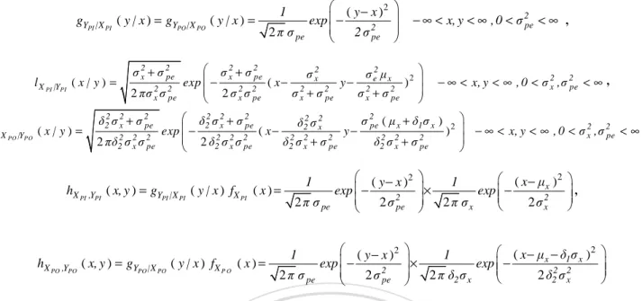
(19) the out-of-control observed quality variable is YPO ~ N ( µx + δ1σx , δ22σx2 + σ 2pe ) . Then the conditional distribution of the observed quality variable Yp given Xp=x is Yp | X p = x ~ N ( x, σ 2pe ) , the in-control conditional distribution of the observed quality variable is YPI | X p = x ~ N ( x, σ 2pe ) , and the out-of-control conditional distribution of the observed quality variable is YPO | X p = x ~ N ( x, σ 2pe ) . The in-control posterior distribution of Xp given YP=y, is X PI |YP = y ~ N (. σ x2 σ x2 + σ 2pe. y+. σ 2pe µx. ,. σ x2 σ 2pe. σ x2 + σ 2pe σ x2 + σ 2pe. (2.1). ). 政 治 And the out-of-control posterior distribution of X given Y =y, is大 立 δ σ σ (µ +δ σ ) δ σ σ p. ‧ 國. 2 pe. x 1 x 2 2 δ2 σ x + σ 2pe. ,. 2 2 2 2 x pe δ22 σ x2 + σ 2pe. ). (2.2). sit. y. Nat. We let. y+. ‧. Note that:. 2 2 2 x δ22 σ x2 + σ 2pe. P. 學. X PO |YP = y ~ N (. (See Appendix A). io. er. f X P I ( x ) , f X P O ( x ) , m Y P I (y ) , m Y P O (y ) , g Y P I | X P I ( y | x ) , g Y P O | X P O ( y | x ) , l X P I |Y P I ( x | y ) ,l X P O |Y P O ( x | y ). al. iv n C h epdf YP respectively for ( x, y ) represent the joint P and i U n gofcXh n. be the density function of XPI, XPO, YPI, YPO, YPI|XPI, YPO|XPO, XPI|YPI and XPO|YPO, respectively, and h X. PI. ,Y P I. ( x, y ) ,h X P O ,Y P O. in-control and. out-of-control processes, where fX PI (x) =. f X PO (x) =. ( x− µx − δ1σ x )2 exp − 2 π δ2 σ x 2 δ22 σ x2 1. mYPI ( y ) =. mYPO ( y ) =. ( x− µx ) 2 exp − 2π σx 2 σ x2 1. . . − ∞ < x < ∞ , − ∞ < µx < ∞ ,0 < σ x2 < ∞ ,. − ∞ < x < ∞ , − ∞ < µx < ∞ ,0 < σ x2 < ∞ , δ1 > 0,δ2 > 1 ,. ( y − µ )2 x −∞ < y < ∞ , −∞ < µx < ∞ ,0 < σ x2 ,σ 2pe < ∞ , exp − 2 2 2 2 2( σ + σ ) 2 π ( σ x + σ pe ) x pe 1. ( y− µ − δ σ )2 x 1 x −∞ < y < ∞ , −∞ < µx < ∞ ,0 < σ x2 ,σ 2pe < ∞ , δ1 > 0,δ2 > 1 , exp − 2 2 2 2 2 2 2 π ( δ2 σx + σ pe ) 2( δ2 σ x + σ pe ) 1. 8.
(20) gYPI |X PI ( y | x ) = gYPO |X PO ( y | x ) =. l X PI |YPI ( x | y ) = l X PO |YPO ( x | y ) =. σ x2 + σ 2pe 2 πσ x2 σ 2pe. δ 22 σ x2 + σ 2pe 2 πδ22 σ x2 σ 2pe. 1 2 π σ pe. ( y − x )2 exp − 2 σ 2pe . . − ∞ < x, y < ∞ , 0 < σ 2pe < ∞. σ x2 + σ 2pe σ2 σ2µ ( x − 2 x 2 y − 2 e x2 ) 2 exp − 2 2 2 σ x σ pe σ x + σ pe σ x + σ pe . ,. − ∞ < x, y < ∞ , 0 < σ x2 ,σ 2pe < ∞ ,. δ22 σ x2 + σ 2pe σ 2pe ( µ x + δ1 σ x ) 2 δ2σ 2 exp − ( x − 2 22 x 2 y − ) − ∞ < x, y < ∞ , 0 < σ x2 ,σ 2pe < ∞ 2 2 2 2 2 2 2 δ2 σ x σ pe + + δ σ σ δ σ σ 2 x pe 2 x pe . hX PI ,YPI ( x, y ) = gYPI |X PI ( y | x ) fX PI ( x ) =. hX PO ,YPO ( x, y ) = gYPO |X PO ( y | x ) fX P O ( x ) =. 1 2 π σ pe. 1 2 π σ pe. ( y − x )2 exp − 2 σ 2pe . ( y − x )2 exp − 2 σ 2pe . ( x − µx ) 2 1 × exp − 2 π σx 2 σ x2 . ,. , . ( x − µ x − δ1 σ x ) 2 1 × exp − 2 π δ2 σ x 2 δ22 σ x2 . . 政 治 大 In complete inspection plan, assume that the producer takes perfect repair or sells at low price for 立. 2.3 Complete Inspection and Adopting Two Actions for Observed Nonconforming Items. nonconforming items. In order to compare the expected profits per unit time of using complete. ‧ 國. 學. inspection plan and process control, we need to derive their profit models.. ‧. 2.3.1 Perfect repair for observed nonconforming items. sit. y. Nat. If the item does not satisfy producer specifications then it will be perfect repaired.. We assume that. io. er. the repaired product would be equal to the target value. The repaired cost per item is assumed to be Cpr.. al. iv n C U target value after repair (i.e. Yr=T). Let Xr beh the of the repaired etrue n gquality c h idistribution n. Because producer only knows the observed quality, the observed quality per item will conform the. nonconforming item. Since Y p = X. p. + ε p , and after repair Yr=T, so Xr = T − ε p ~ N(T , σ 2pe ) .. Figure 2.1 Producer specification based on YP, nonconforming item may perfect repaired with repair cost Cpr. 9.
(21) Figure 2.2 Quadratic loss function based on XP. Assumptions, 1. Let the difference of process mean and target value be µx-T=δσx.. 政 治 大. 2. Producer loss function: Lp=kp(Xp-T)2 When XP is in-control use LPI=kp(XpI-T)2, and XP is out-of-control use LPO=kp(XpO-T)2. 立. 1. f X r (xr )=. 2πσ 2pe. ( x − T )2 exp − r 2 , 2σ pe . 學. ‧ 國. 3. The pdf of Xr is. ‧. and also assume the pdf is the same under process is in-control and out-of-control.. y. Nat. n and for out-of-control Xr, its pdf is. ( x − T )2 exp − r 2 , 2σ pe . er. io. al. 1. f X rI (xr )=. sit. For in-control Xr , its the pdf is,. ni C h2πσ U engchi 2 pe. f X rO (xr )=. 1 2πσ 2pe. ( x − T )2 exp − r 2 2σ pe . 2.3.1-1 Derivation of the profit model per unit time For in-control process, the expected profit per item contains, (1) The sale price for each conforming item is, PPM, (2) The expected loss of a conforming item is, ∞. ∫ ∫. T +dp. −∞ T − d p. LPI hX PI ,YPI (x, y )dydx. 10. v. (2.3).
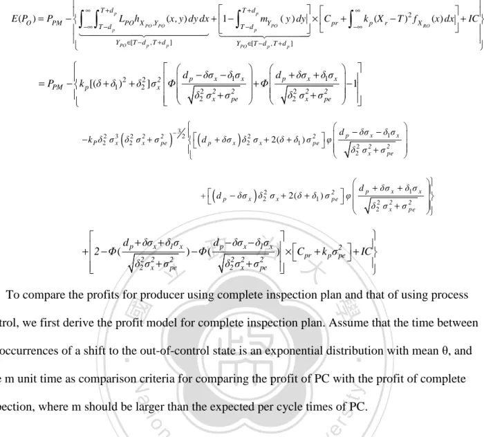
(22) (3) The expected loss of a nonconforming item is, 1− . ∫. T +d p. T −d p. mYPI ( y ) dy × Cpr + . ∞. k p (X r − T )2 f X RI (xr )dxr −∞ . ∫. (4) Inspection cost of an item for producer is, IC.. Hence, the expected in-control profit per item for producer is E(PI), that is, producer selling price minus the cost of producer,. ∫. (. − k P σ 3x σ x2 + σ 2pe. ). −3. 2. 治 政 大 d + δσ . p x +Φ 2 2 σ + σ pe x. . −1 . (. ). (. ) × C pr + k p σ 2pe + IC . ). io. n. er. Nat. d p + δσ x d p − δσ x + 2 − Φ ( ) −Φ( σ x2 + σ 2pe σ x2 + σ 2pe . + d − δσ σ + 2 δ σ 2 φ d p + δσ x p x x pe σ x2 + σ 2pe . ‧. d − δσ x 2 p d p + δσ x σ x + 2 δ σ pe φ σ x2 + σ 2pe . al. k p (X r − T ) 2 f X (xr ) dxr + IC RI . Ch. n engchi U. The expected out-of-control profit per item contains. . y. 立. −∞. 學. d p − δσ x 2 2 − k p (δ + 1) σ x Φ 2 2 σ x + σ pe . ∫. ∞. sit. = PPM. ∫ ∫. ‧ 國. E(PI ) = PPM. ∞ T +d T +d p p − LPI hX ,Y (x, y) dy dx + 1− mY ( y ) dy × C pr + PI PI PI −∞ T −d p T −d p 1444442444443 1444 424444 3 YPI ∈[T −d p ,T +d p ] YPI ∈[T −d p ,T +d p ] . iv. (2.4). (1) The sale price for each conforming item is PPM (2) The expected loss of a conforming item is, ∞. ∫ ∫. T +d p. −∞ T − d p. LPO hX PO ,YPO (x, y )dydx. (3) The expected loss of a nonconforming item is, 1 − . ∫. T +d p. T −d p. mYPO ( y ) dy × C pr + . ∫. ∞. −∞. k p (X r − T )2 f X RO (xr )dxr . (4) Inspection cost of an item for producer is, IC. Hence, the expected out-of-control profit per item for producer E(PO), is producer selling price minus the cost of producer. That is,. 11.
(23) E(PO ) = PPM. = PPM. T +d p ∞ T +d p mY ( y ) dy × C pr + − LPO hX ,Y (x, y) dy dx + 1− PO PO PO −∞ T −d p T −d p 1 44444 42444444 3 1444 424444 3 YPO ∈[T −d p ,T +d p ] YPO ∈[T −d p ,T +d p ] . ∫ ∫. ∫. d p − δσ x − δ1σ x − k p [(δ + δ1 )2 + δ22 ] σ x2 Φ δ22 σ x2 + σ 2pe . (. − k P δ22 σ 3x δ22 σ x2 + σ 2pe. ). −3. + Φ d p + δσ x + δ1σ x δ22 σ x2 + σ 2pe . ∞ k p (X r − T )2 f X (x) dx + IC RO −∞ . ∫. − 1 . d − δσ − δ σ 1 x x 2 2 p d p + δσ x δ2 σ x + 2(δ + δ1 ) σ pe φ 2 2 2 δ2 σ x + σ pe . (. 2. ). . d + δσ + δ σ p x 1 x + d p − δσ x δ 22 σ x + 2( δ + δ1 ) σ 2pe φ δ 22 σ x2 + σ 2pe . (. ). d p + δσ x + δ1σ x d p − δσ x − δ1σ x ) −Φ( + 2 − Φ ( δ22 σ x2 + σ 2pe δ22 σ x2 + σ 2pe . 立. . . 治 ) × C + k σ 政 大. 2 p pe + IC . pr. . To compare the profits for producer using complete inspection plan and that of using process. ‧ 國. 學. control, we first derive the profit model for complete inspection plan. Assume that the time between. ‧. the occurrences of a shift to the out-of-control state is an exponential distribution with mean θ, and. sit. y. Nat. take m unit time as comparison criteria for comparing the profit of PC with the profit of complete. io. n. al. er. inspection, where m should be larger than the expected per cycle times of PC.. Ch. engchi. i Un. v. Figure 2.3 Total profit in m unit time for producer take complete inspection. The expected profit of per time is the sum of the in-control profit in m unit time and out-of-control profit in m unit time divided by m unit time, that is, EPR PIS = 1. R × E ( PI ) ×. 1 1 + R × E ( PO ) × ( m − ) θ θ m. (2.5) Since we also want to compare the yield of perfect repair action and that of sell low price action, we need to calculate the yield. The yield calculation of perfect repair is using the mixture distribution 12.
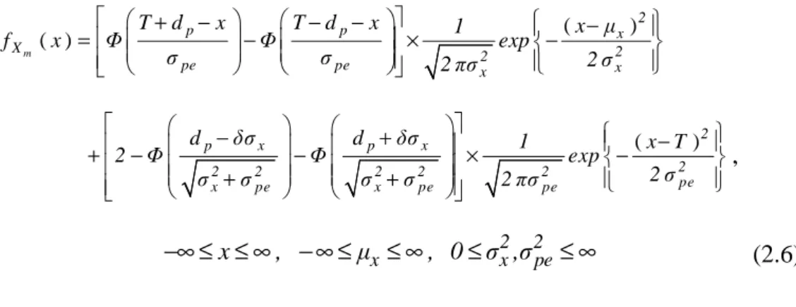
(24) of Xr and XP within specification limits. Therefore, we illustrate the derivation of the mixture distribution as follows, and provide a simulation example to verify the theoretical mixture distribution.. 2.3.1-2 The mixture distribution (Xm) of the true quality (1). The distribution of Xm 2 2 2 2 For X p ~ N ( µx , σx ) and ε p ~ N (0,σ pe ) , then Yp = X p + ε p ~ N ( µx , σx + σ pe ) .. Let. and δ3 =. µ x = T + δσ x. σ x2 σ x2 + σ 2pe. 政 治 大 X ~ N ( T, σ ). The true quality distribution for repaired nonconforming item is,. 立. 2 pe. r. ‧ 國. 學. Then the mixture distribution (Xm) is,. fX ( x) = P(T− dp ≤ Yp ≤ T+ dp )× fX ( x|T− dp ≤ Yp ≤ T+ dp ) +[1− P(T− dp ≤ Yp ≤ T+ dp )]× fX ( x). (. P T − d p ≤ Yp ≤ T + d p. ). ). io. + Φ T − d p − µx × f ( x ) X r σ x2 + σ 2pe . n. al. (. = P X p = x, T − d p ≤ Yp ≤ T + d p. (. Ch. ). engchi. T+ d − µ p x + 1 − Φ 2 2 σ x + σ pe . = P X p = x, T − d p ≤ X p + ε p ≤ T + d p. ). i Un. T+d − µ p x + 1 − Φ 2 2 σ x + σ pe . ). 13. v. + Φ T − d p − µx σ2 + σ2 x pe. d − δσ p x = P T − d p − x ≤ ε p ≤ T + d p − x × f X p (x) + 2 − Φ 2 2 σ +σ x pe. (. y. Nat. T+ d − µ p x + 1 − Φ 2 2 σ x + σ pe . (. P X p = x, T − d p ≤ Yp ≤ T + d p. sit. ). = P T − d p ≤ Yp ≤ T + d p ×. r. ‧. (. P. er. m. × f ( x ) X r . + Φ T − d p − µx σ x2 + σ 2pe . − Φ d p + δσ x 2 2 σ +σ x pe. × f ( x ) X r . (x− T)2 1 × exp − 2 2πσ 2pe 2σ pe .
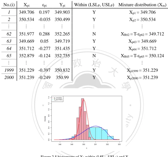
(25) Hence, 2 T+ dp− x T − d p − x 1 ( x − µ x ) f X m ( x ) = Φ exp − −Φ × σ pe 2 σ x2 σ pe 2 πσ x2 . d − δσ p x + 2 − Φ 2 2 σ x + σ pe . − Φ d p + δσ x σ x2 + σ 2pe . × . 1 2 πσ 2pe. . ( x − T ) 2 exp − 2 σ 2pe . , . −∞ ≤ x ≤ ∞ , − ∞ ≤ µx ≤ ∞ , 0 ≤ σ x2 ,σ 2pe ≤ ∞. (2.6). The Figure 2.4 is the pdf for various value of Xm under T=350, δ = 1, δ3 = 95.78%, σx = 1 and dp* = 2.24.. 立. 政 治 大. ‧. ‧ 國. 學. n. er. io. sit. y. Nat. al. i n C Figure 2.4 The pdf X U hengchi. v. m. (2). Simulation example 2 . %, Let Target value (T) =350, δ =1, σx =1, δ3 = 9578 2 2 2 That is, X p ~ N ( µx = 352, σx = 1) and ε p ~ N (0, σ pe = 0.3 ). 2 2 Then Yp = X p + ε p ~ N ( µx = 352, σx + σ pe = 1.09). Suppose that dp*=2.24, then we have (LSLP, USLP) = (T-dp*, T+dp*) = (347.76, 352.24) We simulate 2000 data from distribution of XP and εp, then the 2000 values of YP are obtained (See Table 2.1).. 14.
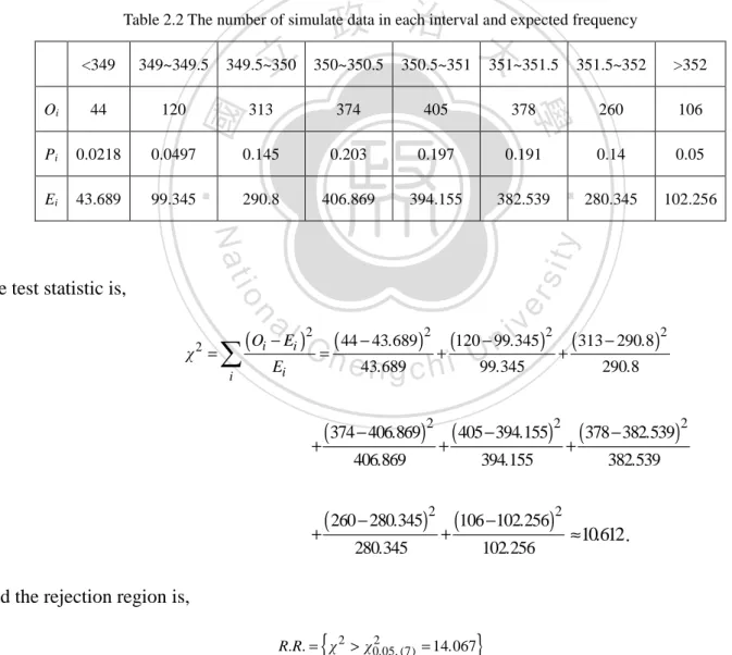
(26) Figure 2.5 illustrates the histograms of XP within (LSLP, USLP) and Xr , and Figure 2.6 illustrates the histogram and theorical curve of mixture distribution.. Table 2.1 Numeric example for finding true quality distribution (XM) of products received by middleman. No.(i). Xpi. εpi. Ypi. 1. 349.706. 0.197. 349.903. Y. Xp1 = 349.706. 2. 350.534 -0.035 350.499. Y. Xp2 = 350.534. Within (LSLP, USLP) Mixture distribution (Xm). M. M. M. M. M. M. 62. 351.977. 0.288. 352.265. N. XR62 = T-εp62 = 349.712. 63. 349.669. 0.05. 349.719. Y. Xp63 = 349.669. 64. 351.712 -0.277 351.435. Y. Xp64 = 351.712. 65. 352.879 -0.124 352.755. N. XR65 = T-εp65 = 350.124. M. M. M. M. 1999. 351.229 -0.397 350.832. 2000. 351.239 -0.249. 立. M 政 治 大 Y. 350.99. M. Xp1999 = 351.229. Y. Xp2000 = 351.239. ‧. ‧ 國. 學. n. er. io. sit. y. Nat. al. Ch. engchi. i Un. v. Figure 2.5 histograms of XP within (LSLP, USLP) and Xr. Figure 2.6 histogram of mixture distribution and theorical curve. 15.
(27) Now we apply the goodness of fit to prove that the data in Table 3.1 has the same distribution as in (2.6). First we states the null hypothesis and the alternate hypothesis, H0︰The data follows the mixture distribution H1︰The data do not follows the mixture distribution And we select the significant levels, α = 0.05 in this problem. Then we cut the data into eight intervals, and count the number in each interval, also use the mixture distribution to calculate the expected frequency in each interval.. 政 治 大 350~350.5 350.5~351 351~351.5. Table 2.2 The number of simulate data in each interval and expected frequency. 立. Oi. 44. 120. 313. 374. 405. Pi. 0.0218. 0.0497. 0.145. 0.203. Ei. 43.689. 99.345. 290.8. 406.869. ‧ 國. 349.5~350. 351.5~352. >352. 378. 260. 106. 0.197. 0.191. 0.14. 0.05. 394.155. 382.539. 280.345. 102.256. ‧. 349~349.5. 學. <349. er. io. sit. y. Nat. The test statistic is,. a. v. n. χ = 2. ∑ i. 2 2 2 2 44 − 43.689 ) 120 − 99 .i345 ) 313 − 290.8 ) ( Oi − El i )C ( ( ( n = + +. Ei. h e43n.689 g c h i U99.345. 290.8. 2 2 2 374 − 406.869) ( 405 − 394.155) ( 378 − 382.539) ( + + +. 406.869. 394.155. 2 2 260 − 280.345) (106 −102.256) ( + +. 280.345. 102.256. 382.539. ≈10612 . .. And the rejection region is,. {. }. R.R. = χ 2 > χ 02.05 , (7) = 14.067. 2 Since χ ≈10.612∉R.R. , so we do not reject H0, that is, we do not have sufficient evidence to say this. simulate data do not follows the mixture distribution.. 16.
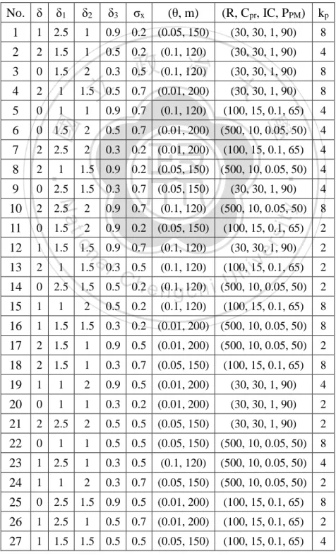
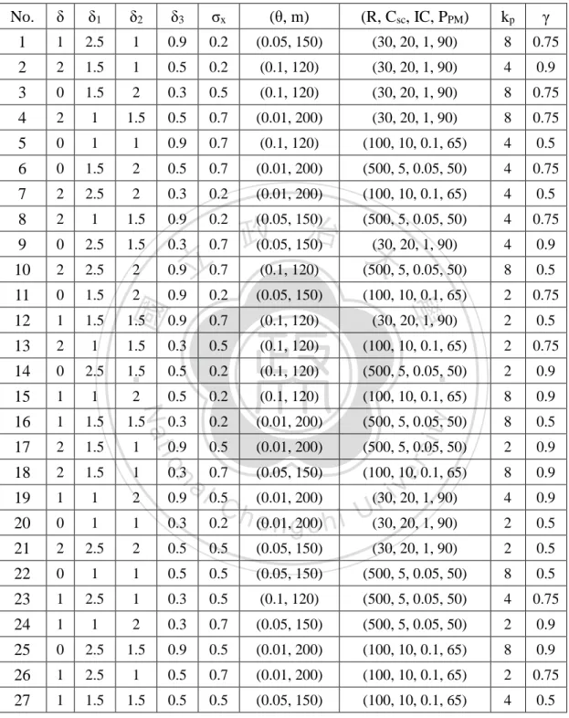
(28) After having the mixture distribution, then we may calculate its yield (see (2.7)). .. (. ) ∫. P T − d *p ≤ X m ≤ T − d *p =. T − d *p. ∫. =. T + d *p. T + d *p. T. − d *p. f X m ( x ) dx. T + d* − x T − d *p − x p Φ −Φ × σ pe σ pe . d * − δσ p x + 2 − Φ 2 2 σ + σ x pe d *p − δσ x. ∫. =. −. σx d *p + δσ x σx. d * − δσ σ x Φ p − x σ pe σ pe . d* − δσ p x + 2 −Φ 2 2 σ +σ x pe . × . * − Φ d p + δσ x σ x2 + σ 2pe . 2 πσ x2. ∫. T + d *p. T − d *p. 2 ( x − µ x ) exp − dx 2 2 σ x . 1 2 πσ 2pe. d *p + δσ x σ z+Φ + x σ pe σ pe . * − Φ d p + δσ x 2 2 σ +σ x pe. × . 政 治 大. 立. 1. d*p +δσ x. ∫. −. σx d*p + δσ x σx. 2 ( x − T ) exp − 2 σ 2pe . dx . z − 1 × φ ( z ) dz . σx 2πσ 2pe. σ 2 ( z+ δ)2 exp − x 2 dz 2σ pe . (2.7). Table 2.3 Three Levels of Each Parameters. y. Nat. Level 2. δ δ1 δ2 δ3 σx (θ, m) kp. 0 1 1 0.3 0.2 (0.01, 200) 2. 1 1.5 1.5 0.5 0.5 (0.05, 150) 4. (500, 10, 0.05, 50). (100, 15, 0.1, 65). 3. 2 2.5 2 0.9 0.7 (0.1, 120) 8. er. n. Ch. sit. 1. io. parameter. (R , Cpr , IC , PPMH). ‧. ‧ 國. 學. 2.3.1-3 Determine the optimal inspection specification limits and data analyses. al. engchi. i Un. v. (30, 30, 1, 90). Since 8 parameters each with 3 levels, the parameters could be assigned to each combination of. ( ). 13 orthogonal array table L27 3 (see table 2.4).. 17. ,.
(29) Let the expected profit of per time under producer taking perfect repair for nonconforming item is. EPRPIS . To determine optimal producer specification limits, we maximize EPRPIS with the constraint 1 1 0 ≤ d p ≤ 3 σ x2 + σ 2pe. by using “optim” routine in R program, where σ x2 + σ 2pe. of YP, and here use three times. σ x2 + σ 2pe. two actions than use six times. σ x2 + σ 2pe. is the standard deviation. is because it can more easy to find profit difference in the. . 13. Table 2.4 The 27 combinations of these parameters by using an orthogonal array table L27 (3 ) .. δ1. δ2. δ3. 1. 1 2.5. 1. 2. 2 1.5. 3. 0 1.5. 4. 2. 1. 5. 0. 1. 6. 0 1.5. 2. 0.5 0.7 (0.01, 200) (500, 10, 0.05, 50). 4. 7. 2 2.5. 2. 0.3 0.2 (0.01, 200). (100, 15, 0.1, 65). 4. 8. 2. 1.5 0.9 0.2 (0.05, 150) (500, 10, 0.05, 50). 4. 9. 0 2.5 1.5 0.3 0.7 (0.05, 150). 10. 2 2.5. 2. 0.9 0.7. 11. 0 1.5. 2. 12. 1 1.5 1.5 0.9 0.7. 13. 2. 14. 0 2.5. (R, Cpr, IC, PPM). kp. 0.9 0.2 (0.05, 150). (30, 30, 1, 90). 8. 1. 0.5 0.2. (30, 30, 1, 90). 4. 2. 0.3. 大 (30, 30, 1, 90). 8. (100, 15, 0.1, 65). 4. 立. (θ, m) (0.1, 120). 政(0.1, 治 0.5 120). 1. 0.9 0.7. (0.1, 120). (30, 30, 1, 90). ‧. 4. (0.1, 120). (500, 10, 0.05, 50). y. 8. 0.9 0.2 (0.05, 150). (100, 15, 0.1, 65). 2 2. 15. 1. a 1.5 l0.3 0.5 (0.1, 120) (100, 15, i v 0.1, 65) n C U 10, 0.05, 50) h e n(0.1,g 120) 1.5 0.5 0.2 c h i (500, (100, 15, 0.1, 65). 8. 16. 1 1.5 1.5 0.3 0.2 (0.01, 200) (500, 10, 0.05, 50). 8. 17. 2 1.5. 1. 0.9 0.5 (0.01, 200) (500, 10, 0.05, 50). 2. 18. 2 1.5. 1. 0.3 0.7 (0.05, 150). (100, 15, 0.1, 65). 8. 19. 1. 1. 2. 0.9 0.5 (0.01, 200). (30, 30, 1, 90). 4. 20. 0. 1. 1. 0.3 0.2 (0.01, 200). (30, 30, 1, 90). 2. 21. 2 2.5. 2. 0.5 0.5 (0.05, 150). (30, 30, 1, 90). 2. 22. 0. 1. 0.5 0.5 (0.05, 150) (500, 10, 0.05, 50). 8. 23. 1 2.5. 1. 0.3 0.5. (500, 10, 0.05, 50). 4. 24. 1. 2. 0.3 0.7 (0.05, 150) (500, 10, 0.05, 50). 2. 25. 0 2.5 1.5 0.9 0.5 (0.01, 200). (100, 15, 0.1, 65). 8. 26. 1 2.5. 0.5 0.7 (0.01, 200). (100, 15, 0.1, 65). 2. 27. 1 1.5 1.5 0.5 0.5 (0.05, 150). (100, 15, 0.1, 65). 4. Nat. (30, 30, 1, 90). sit. 8. er. 學. 1. σx. 1.5 0.5 0.7 (0.01, 200). ‧ 國. No. δ. io. n. 1 1. 1 1. 2. 1. 0.5 0.2. (0.1, 120). (0.1, 120). (0.1, 120). 18. (30, 30, 1, 90). 2 2.
(30) Table 2.5 The optimal solutions of the 27 combinations of parameters No.. 1. d *P. EPR*PIS. Yield for Xr and XP within. Yield for Yr and YP within. producer specification. producer specification. 99.72225. 100. 1. 0.667 2199.665. 2. 1.2. 2528.73. 99.99737. 100. 3. 5. 2318.279. 99.99955. 100. 4. 2.862 1840.306. 98.95622. 100. 5. 2.236 6123.522. 99.95584. 100. 6. 2.866 22048.36. 99.92446. 100. 99.99861. 100. 7 8 9. 2. 6216.319. 0.667 22837.61 7. 2222.793. 立. 97.87574治 政 大 99.99955. 100 100. 92.5609. 100. 11. 0.667 6216.334. 99.97256. 100. 12. 2.333 2332.112. 99.72225. 14. 1.2. 15 16. 99.99861. 24410.14. 99.99986. 1.2. 6203.725. 99.99964. 100. 2. 24093.03. 99.99934 97.87574. 100. y. 100. sit. Nat. 5933.368. ‧. 5. 100. io. 13. ‧ 國. 0.985 19786.47. 學. 10. 100. 1.667 22401.67. 18. 4.124 1854.804. 19. 1.667. 2477.111. 20. 2. 2663.354. 21. 3. 2264.429. 99.99737. 100. 22. 3. 23098.93. 99.99986. 100. 23. 5. 18797.83. 99.99934. 100. 24. 6.961 21475.07. 99.99927. 100. 25. 1.41. 5866.42. 99.85492. 100. 26. 4.2. 5746.94. 99.99964. 100. 27. 3. 5742.331. 99.99964. 100. n. al. 99.16414. C h99.72225 i U e h n c g 99.99955. 19. er. 17. v ni. 100 100 100 100.
(31) The response figure and table are applied to find the significant parameters of d*P and EPR*PIS1 .. (I) Response figure and table of d*P. 治 政 Figure 2.7 Response figure of d for each 大parameter 立 學. * Table 2.6 Table Response table of dP. δ1. δ2. δ3. σx. (θ, m). (R, Cpr, IC, PPM). kp. 2.705 2.649 2.859. 3.003 2.848 2.361. 0.21. 0.642. ‧. δ. ‧ 國. * P. n. al. Ch. engchi. sit. 0.614 0.304 0.153 2.976 2.441 0.935. er. io. diff. y. Nat. level1 2.82 2.844 2.677 4.343 1.289 2.297 level2 3.003 2.54 2.83 2.503 3.194 3.232 level3 2.389 2.829 2.705 1.367 3.73 2.684. i Un. v. Based on the Table 2.6, if the difference between maximal and minimal values of the three levels is larger than 1.5, the parameters, δ3 and σx are determined to be significant in relation to d*P . The optimal producer specification is determined by the constraint of the variance of observed quality characteristics, σ2x + σ2pe . Therefore, δ3 and σx are significant parameters of d*P , and the δ3 and σx trends are, (1) when δ3 increases then d*P decreases. (2) when σx increases then d*P increases.. 20.
(32) (II) Response figure and table of EPR*PIS1. Figure 2.8 Response figure of EPR* PIS1 for each parameter. 立. 政 治 大. 學. δ. ‧ 國. Table 2.7 Response table of EPR* PIS1. δ1. δ2. δ3. σx. (θ, m). (R, Cpr, IC, PPM). kp. 10294.78. 9490.604. 9508.316. 10818.77. 10372.61. 22105.46. 10382.6. 9896.423. 9948.406. 10586.46. 10431.54. 9877.818. 9767.996. 5544.863. 9888.289. 9518.19. 9723.445. 9889.566. 10026.77. 9270.042. 9826.019. 2316.309. 9695.736. diff. 1033.823. 571.333. 923.227. 1548.726. 604.616. 19789.15. 686.865. y er. io. sit. 1095.853. ‧. 10552.01. Nat. level1 level2 level3. Based on Table 2.7, if the difference between the maximal and minimal values of the three levels. al. n. iv n C is larger than 3000, the parameter (R, Cpr, IC,hPPM e )nisgdetermined c h i Uto be significant for. EPR*PIS1 .. When (R, Cpr, IC, PPM), increases EPR*PIS1 decreases. Although PPM increases between the three levels, but the difference in PPM value is not large. Moreover, R decreases between the levels, but the difference in R value is large. Therefore EPR*PIS1 is significantly affected by the amount of production (R). This means when per item profit is small, the producer should adopt mass production to increase profit.. 21.
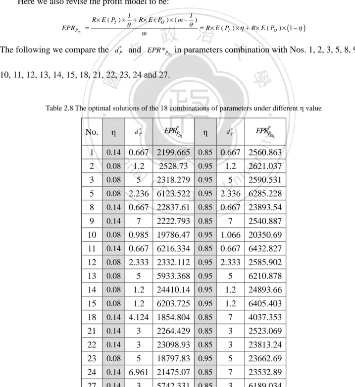
(33) In 2.3.1-3 data analyses, the parameter combination of (θ, m) may relate to the time of in-control and out-of-control process, and the ratio of 1/θ to m is the proportion of expected in-control time to the m unit time, here denoted by η. The expected in-control time can’t be shorter than out-of-control time, that is, η should be larger than 0.5. But in the data analysis there are two parameter combination of (θ, m), (0.05, 150) and (0.1, 120) are not appropriate, since the η values are 0.14 and 0.08 respectively, so here we change the η value to be 0.85 and 0.95 to find whether the optimal specification limits and the EPR*PIS. 1. may be changed or not.. Here we also revise the profit model to be: EPR PIS =. R × E ( PI ) ×. 1. 1 1 + R× E ( PO ) × ( m − ) θ θ = R × E ( P ) × η + R× E ( P ) × (1 − η ) I O m. The following we compare the d *P and. 立. 政 治 大 EPR* in parameters combination with Nos. 1, 2, 3, 5, 8, 9, PIS1. ‧ 國. 學. 10, 11, 12, 13, 14, 15, 18, 21, 22, 23, 24 and 27.. d *P. η. EPR*PIS. η. EPR*PIS. d *P. 2. 0.08. 3. 0.08. 5. 0.08. 8. 0.14 0.667 22837.61 0.85 0.667 23893.54. 9. 0.14. 10. 0.08 0.985 19786.47 0.95 1.066 20350.69. 11. 0.14 0.667 6216.334 0.85 0.667 6432.827. 12. 0.08 2.333. 13. 0.08. 5. 5933.368 0.95. 5. 6210.878. 14. 0.08. 1.2. 24410.14 0.95. 1.2. 24893.66. 15. 0.08. 1.2. 6203.725 0.95. 1.2. 6405.403. 18. 0.14 4.124 1854.804 0.85. 7. 4037.353. 21. 0.14. 3. 2264.429 0.85. 3. 2523.069. 22. 0.14. 3. 23098.93 0.85. 3. 23813.24. 23. 0.08. 5. 18797.83 0.95. 5. 23662.69. 24. 0.14 6.961 21475.07 0.85. 7. 23532.89. 27. 0.14. 3. 6189.034. 1. sit. 1. y. 1. Nat. No.. ‧. Table 2.8 The optimal solutions of the 18 combinations of parameters under different η value. n. a1.2l. 2528.73. 0.95. 1.2. er. io. 0.14 0.667 2199.665 0.85 0.667 2560.863 0.95 5n C2318.279 U h e n g c0.95h i 2.336 2.236 6123.522. 5. 7. 3. 2222.793 0.85. 7. 2621.037. i v2590.531 6285.228 2540.887. 2332.112 0.95 2.333 2585.902. 5742.331 0.85 22.
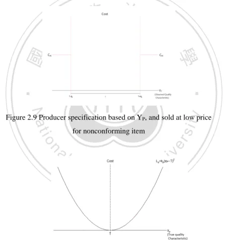
(34) From the Table 2.8, we found that, 1. the optimal specification limits width became wider in Nos. 10, 18, 24, and for others the optimal specification limits are the same. 2. EPR*PIS1 is larger for high η value.. 2.3.2 Taking sell low price action for observed nonconforming items. If the quality of the product satisfies the producer’s specifications, then it will be sold at a high price, (PPMH). However, if the quality does not satisfy the producer’s specifications, then the cost of the nonconforming item (Csc) is involved, and the product will be sold at low price, (PPML > Csc).. 立. 政 治 大. ‧. ‧ 國. 學 y. Nat. for nonconforming item. n. al. er. io. sit. Figure 2.9 Producer specification based on YP, and sold at low price. Ch. engchi. i Un. v. Figure 2.10 Quadratic loss function based on XP. 23.
數據
+7
Outline
INTRODUCTION
Perfect repair for observed nonconforming items
Taking sell low price action for observed nonconforming items
Comparing the Expected Profit Per Unit Time for Complete Inspection Plan and Process Control
Derivation of the profit model for middleman
Comparing the four cases expected profit of middleman for middleman instrument with
Comparing the middleman ordered quantity and middleman profit for middleman instrument
SUMMARY AND FUTURE STUDY
相關文件
Transfer of training: A review and directions for future research. (1992).“Formal and
As the result, I found that the trail I want can be got by using a plane for cutting the quadrangular pyramid, like the way to have a conic section from a cone.. I also found
Step 1: With reference to the purpose and the rhetorical structure of the review genre (Stage 3), design a graphic organiser for the major sections and sub-sections of your
LinkedIn, 2019 & 2020, The skills that employers most looking for Ministry of Education and Research, Norway 2010, Action Plan – Entrepreneurship in Education and Training –
1.5 In addition, EMB organised a total of 58 forums and briefings (45 on COS and 13 on special education) to explain the proposals in detail and to collect feedback from
The new academic structure for senior secondary education and higher education - Action plan for investing in the future of Hong Kong.. Hong Kong: Education and
This paper presents (i) a review of item selection algorithms from Robbins–Monro to Fred Lord; (ii) the establishment of a large sample foundation for Fred Lord’s maximum
The person making the measurement then slowly lowers the applied pressure and listens for blood flow to resume. Blood pressure sure pulsates because of the pumping action of the
