國
立
交
通
大
學
資訊學院資訊科技(IT)產業研發碩士班
碩
士
論
文
具 有 優 先 權 特 性 之 移 動 式 感 測 器 派 遣 方 法 的 設 計 與 建 置
Design and Implement Priority-Based Dispatch of Mobile Sensors in
Surveillance Applications
研 究 生:王文杰
指導教授:曾煜棋 教授
具有優先權特性之移動式感測器派遣方法的設計與建置
Design and Implement Priority-Based Dispatch of Mobile Sensors in
Surveillance Applications
研 究 生:王文杰 Student:Wen-Chieh Wang
指導教授:曾煜棋 Advisor:Yu-Chee Tseng
國 立 交 通 大 學
資訊學院資訊科技(IT)產業研發碩士班
碩 士 論 文
A ThesisSubmitted to College of Computer Science National Chiao Tung University in partial Fulfillment of the Requirements
for the Degree of Master
in
Industrial Technology R & D Master Program on Computer Science and Engineering
June 2008
Hsinchu, Taiwan, Republic of China
具 有 優 先 權 特 性 之 移 動 式 感 測 器 派 遣 方 法 的 設 計 與 建 置
學生:王文杰
指導教授:曾煜棋
國立交通大學資訊學院產業研發碩士專班
摘
要
無線感測器網路的使用提供一個方便的方式來監控環境。但其並非一定會在
我們關注的區域部署感測器,而在這樣的情形下,如何獲得環境狀態是一個很大
的挑戰。在本篇論文中,我們嘗試利用移動式感測器在沒有部署感測器網路的待
測環境中快速並詳細的得知事件的發生。在這樣的動作中會要求移動式感測器對
環境作全區域的掃描,藉此發現事件在哪裡發生,之後再派遣感測器到事件的發
生地作更進一步的資料收集。我們在移動式感測器上使用一個以優先權為基礎的
派遣方式,接著我們會根據事件發生的位置與事件本身的優先權定義作為拜訪事
件時的判斷條件,若事件的優先權較高且移動距離較短者將優先拜訪。在這樣的
定義下,移動式感測器將能快速完成他們的工作並且更重要的事件也能在消失前
優先分析。我們建立了一個系統驗證我們的派遣方法。模擬的結果也呈現這個方
法的效果。
Design and Implement Priority-Based Dispatch of Mobile Sensors in Surveillance
Applications
student:Wen-Chieh Wang Advisors:Dr. Yu-Chee Tseng
Industrial Technology R & D Master Program of
Computer Science College
National Chiao Tung University
ABSTRACT
Wireless sensor networks provide a convenient way to monitor the physical environment.
However, it is not always possible to have a deployment of a sensor network in the region of
interest. In this case, how to obtain the environmental situations is a big challenge. In this
paper, we propose to use mobile sensors to quickly capture and analyze the events occurred in
a region without any deployment of sensor networks. The idea is to request mobile sensors to
fully scan the environment to find out where events occur and then dispatch mobile sensors to
event locations to conduct more advanced data collections. We propose a priority-based
dispatch scheme for mobile sensors to visit events according to events' locations and priorities.
In particular, events with higher priorities and shorter moving distances will be visited first. In
this way, mobile sensors can quickly finish their jobs and the most important events can be
analyzed earlier before they disappear. We have implemented a prototyping system to
demonstrate our dispatch idea. Simulation results are also presented to verify the effectiveness
of the proposed schemes.
誌
謝
首先,要先感謝的是我的指導教授曾煜棋老師,在相關的方面給我很大的空間,並且在論文的寫作過程中給予相當多 的幫助,並且也幫忙我修正論文表達以及寫作方面的問題。接著要感謝的是帶我的王友群學長,如果沒有學長從旁的協助 和提攜,論文是沒有辦法能這麼順利的在時間內完成。再者要感謝胡淑琼學姐、李祖光學長、黃全淯學弟等,在論文討論 的過程中給予許多的想法、建議和協助,讓我能看見論文本身許多的問題進而修改的更好。另外,就是潘孟鉉學長、蔡佳 宏學長點出論文內容的諸多問題,並且建議要如何修改,也才有現在的論文。再來就是家人的支持,原本家裡並不是那麼 認同我放棄工作回到學校讀書的作法,但之後慢慢接受,並且認同我的想法和作法,我很感謝。最後,就是要感謝所有曾 經參與和幫助過我的各位,有你們才能讓我完成這件工作,謝謝。 對於工作了一段時間後又再度回到學校的我來說,在剛進來的時候對於研究領域的相關並不是那樣的清楚,加上離開 學校有一段時間,對於學校的一切是陌生、未知和戒慎恐懼的。直到論文完成的現在其實還是有點不敢置信。因為是技職 體系學生的關係,在這段時間中的學習一直都有別於以前,可以說是類似但方向不同的一種觀念,使得我在看待事情上多 擁有了不同於以往的思考角度和建構方法,我想這會是我所得到最重要的。
Contents
Chinese Abstract i English Abstract ii Acknowledgement iii Contents iv List of Figures vi 1 Introduction 1 2 Preliminary 6 2.1 Problem Statement . . . 6 2.2 Related Works . . . 83 A Priority-Based Dispatch Scheme 10
3.2 Finding a Suitable Hamilton Cycle . . . 14 3.3 Time Complexity Analysis . . . 17
4 Prototyping Experiences 19
4.1 Hardware Specifications . . . 20 4.2 User Interface at the Control Server . . . 23
5 Simulation Results 29
6 Conclusions 33
List of Figures
2.1 An example to model the environment: (a) sensing field A
with obstacles and (b) logically dividing A into grids. . . . 7
3.1 An example to calculate the shortest distance between two locations lS and lD. . . 14
3.2 An example to show how to find the Hamilton cycle with the minimum cost. . . 17
4.1 The mobile sensor. . . 22
4.2 The operating flowchart of the mobile sensor. . . 23
4.3 A 9 × 5 grid-like sensing field in our experiment. . . 24
4.4 User interface at the control server. . . 25
4.5 The DHCP server. . . 26
4.6 The map editor. . . 27
4.7 Snapshots of the user interface when executing the priority-based dispatch scheme. . . 28
5.1 Comparison on the total moving time of the mobile sensor. . . 30 5.2 Comparison on the costs of the Hamilton cycles. . . 31 5.3 Waiting time of event locations. . . 32
Chapter 1
Introduction
Recently, mobile sensors have attracted a lot of attentions by researchers. By mounting sophisticated sensing devices on mobile platforms [1–3], we can move these mobile sensors to conduct sensing missions at certain locations. With mobility, mobile sensors can significantly extend the capability of sensor networks.
In this thesis, we consider how to quickly obtain the events occurred in a region without any pre-deployment of sensor networks. This issue is quite im-portant for those surveillance applications in some harsh environments where it is difficult to deploy static sensors in advance. Under such a scenario, one possible solution is to dispatch mobile sensors to collect rough environmen-tal information and then carefully analyze events later. In particular, we first request mobile sensors to fully scan the environment to collect basic
information of events (e.g., locations and priorities). Then, we can dispatch mobile sensors to visit these events to conduct more advanced analysis. For example, one can imagine a surveillance application to detect gas leakage in an airtight factory without deployment of sensor networks. We can dispatch mobile sensors to fully scan the factory to collect the densities of gas in differ-ent locations and find out potdiffer-ential sources of leakage. Then, mobile sensors can be dispatched to these sources to obtain more detailed information.
Given the priorities of event locations, it is a critical issue to efficiently dispatch a mobile sensor to visit all event locations such that the total moving time of the mobile sensor is minimized and the event locations with higher priorities can have a shorter waiting time, where the waiting time of an event location is defined as the duration until the mobile sensor reaches that location. Clearly, we should reduce the total moving time of the mobile sensor so that events can be quickly analyzed to satisfy the requirements of surveillance applications. On the other hand, since events may disappear in short time, the mobile sensor should first visit event locations with higher priorities earlier.
In the literature, a large amount of researches on mobile sensors have fo-cused on how to use mobile sensors to deploy a sensor network [4–7], how to enhance the network coverage [8], and how to improve the network connec-tivity [9]. The work in [10] discusses how to move more mobile sensors close
to event locations, but it focuses on maintaining complete coverage of the sensing field. Several studies [11, 12] implement the pursuer-evader game by a sensor network, where a pursuer (i.e., a mobile sensor) needs to intercept an evader (i.e., a moving object) by the assistance of a static sensor net-work. However, these works focus on how to quickly tell the pursuer where the evader is through the sensor network. Some works [13, 14] consider to dispatch mobile sensors to visit events in a sensor network consisting of both static and mobile sensors. In [13], static sensors that have detected events will invite and navigate nearby mobile sensors to move to their locations. The mobile sensor that has shorter moving distance and more energy, and whose leaving will not cause a large coverage hole, will be invited by the static sensors. The work in [14] addresses how to balance the loads of mobile sensors when dispatching them to visit event locations, so that the system lifetime of mobile sensors can be extended. However, these works assume that events have the same importance, so their results may not be directly applied to our sensor dispatch problem.
In this thesis, we propose a priority-based dispatch scheme for mobile sensors to visit event locations. Given an environment with obstacles, we first request mobile sensors to fully scan the environment to obtain the lo-cations and priorities of events. Then, we dispatch mobile sensors to visit and carefully analyze these events based on their locations and priorities. In
particular, the dispatch problem can be viewed as a variance of the traveling salesman problem (TSP) that considers the priorities of visiting locations. Since TSP is NP-complete, we thus propose a heuristic approach to effi-ciently calculate the dispatch schedule of mobile sensors. We also develop a prototyping system to demonstrate our dispatch idea. This prototype is used to monitor the densities of carbon dioxide (CO2) in an indoor environ-ment. Specifically, we mount CO2 sensing devices on a mobile platform and dispatch these mobile sensors to monitor CO2 densities and to analyze po-tential CO2 sources. Simulations are also conducted to validate the efficiency of our dispatch scheme in a large-scale scenario.
Major contributions of this thesis are two-fold. First, our proposed dis-patch scenario allows people to monitor and analyze important events oc-curred in a region with obstacles, even though there is no infrastructure of sensor networks inside that region. By dispatching mobile sensors to fully scan the region and visit event locations based on their locations and prior-ities, we can quickly assess the whole environment situation. This may be especially helpful for rescuing applications in some hazardous regions. Sec-ond, we implement a prototyping system to realize our dispatch idea. This prototype system also demonstrates a surveillance application to monitor the CO2 densities in an indoor environment.
the dispatch problem and reviews some related works. Section 3 proposes our priority-based dispatch scheme. Section 4 shows our prototyping experiences. Section 5 gives some simulation results. Section 6 concludes this thesis.
Chapter 2
Preliminary
2.1
Problem Statement
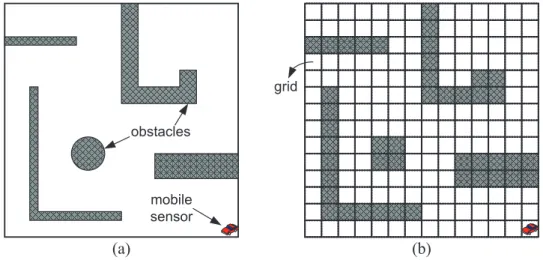
We consider a sensing field A possibly with obstacles, as shown in Fig. 2.1(a). We assume that these obstacles do not partition A. Otherwise, full scan-ning wouldn’t be possible. For convenience, we logically divide A into small squares (called grids). In this way, obstacles can be modeled by grids (marked by gray in Fig. 2.1(b)). Mobile sensors will patrol inside A along these grids to conduct full scanning and to visit event locations. Each mobile sensor has four basic moving patterns: east, west, north, and south, where the mobile sensor will move toward the specified direction with one-grid length. Moving from one grid to another will take ∆m time to finish. The other four diagonal
requires ∆t time for a mobile sensor to make a 90-degree turn. obstacles mobile sensor grid (a) (b)
Figure 2.1: An example to model the environment: (a) sensing field A with obstacles and (b) logically dividing A into grids.
We assume that after a mobile sensor fully scans A, we can obtain a set of event locations L = {(l1, p1), (l2, p2), · · · , (ln, pn)}, where li = (xi, yi) and
pi > 0 are the location and priority of an event i, respectively. A smaller
value of pi means a higher priority. Note that two events may have the same
priority. Our sensor dispatch problem is stated as follows: Given a mobile sensor initially located at l0 = (x0, y0) and the set L, how to dispatch the mobile sensor to visit all locations in L such that the total moving time of the mobile sensor is minimized and event locations with higher priorities can have shorter waiting time.
scan the sensing field A and the time to detect events. Since fully scanning A requires the mobile sensor to visit every grid inside A and the time to analyze an event depends on the sensing capability of the mobile sensor, we thus ignore these two latencies. In addition, we focus on the dispatch problem of one mobile sensor. In the case of multiple mobile sensors, we can partition A into multiple non-overlapped subregions and then dispatch one mobile sensor to travel inside each subregion.
2.2
Related Works
Our dispatch problem can be viewed as a TSP variance that considers the priorities of visiting locations. TSP is one of the famous NP-complete prob-lems and there have been many approximation solutions proposed to solve it and its variances [15]. Given an undirected weighted graph G = (V, E), TSP asks how to find a Hamilton cycle C on G such that the total edge weight of C can be minimized. To solve TSP, Blaser [16] suggests that we can first find the minimum spanning tree on G and then visit all vertices in V by a pre-order tree walk of the spanning tree. The visiting sequence of vertices is the approximate solution of TSP. Some works adopt more sophisticated methods to solve TSP. For example, Zhu and Chen [17] solve TSP by simulating ants’ behaviors. In particular, each time when an ant passes through a path, it
will leave pheromone along that path. Such pheromone will attract other ants to walk through this path. Thus, when a path is walked by more ants, it will have a larger amount of pheromone. By adopting this concept, we can first try some paths to visit vertices in the graph. When a “good” path is found, it will leave more pheromone and thus attracts more ants to walk through it. Finally, the path with the most pheromone will be the solution. Other works use simulated annealing [18], genetic algorithm [19], and tabu search method [20] to solve TSP. Obviously, these methods can approximate a better solution, but they may suffer from a higher computation cost.
On the other hand, several works consider the variances of TSP. The work in [21] introduces the concept of time window to TSP, where each location is associated with a time duration where we expect the salesman will visit that location within the specified time duration. This can be applied to some applications with timetables such as bus scheduling or consignment of goods. The work [22] considers a dynamic environment, where visiting locations may be disappeared or changed as time goes by. This can be used in some applications like realtime computing in satellite systems. Given a set of locations L, the work [23] considers how to visit locations in L with a minimum cost, where a subset L0 ⊆ L of locations may follow some
probability model. As can be seen, the solutions of these works may not be directly applied to our problem.
Chapter 3
A Priority-Based Dispatch
Scheme
Given the sensing field A and a mobile sensor initially located to l0, our priority-based dispatch scheme involves the following steps:
1. Dispatch the mobile sensor to visit all grids in A to collect locations and rough information of events in L. To conduct such a full scanning, we can adopt the solutions proposed in [24].
2. Calculate the shortest distance d(li, lj) between any two locations li and
lj, where li and lj ∈ L ∪ {l0}. Note that the above calculation should consider the existence of obstacles. How to calculate d(li, lj) will be
3. Construct a weighted complete graph G = (V, E), where V = L ∪ {l0}. For each vertex li ∈ L, we associate it with a priority value pi. How
to assign the priority depends on the application requirement. One possible assignment is based on events’ strengths (e.g., gas’s densities). The weight wi,j of each edge (li, lj) ∈ E is defined as the moving time
for a mobile sensor to move along the shortest distance d(li, lj).
4. Find a Hamilton cycle (l0, lv1, lv2, · · · , lvn, l0) on G to minimize
w0,v1 + n−1 X i=1 wvi,vi+1+ wvn,0, (3.1) such that x−1 X i=1 wvi,vi+1 ≤ y−1 X i=1 wvi,vi+1, ∀pvx ≤ pvy. (3.2)
Eq. (3.1) means that we should minimize the total moving time for the mobile sensor to visit all event locations, and Eq. (3.2) indicates that an event location lvx with a higher priority should have smaller waiting
time compared with another event location lvy with a lower priority.
Note that we eliminate the term w0,v1 from both the left and right
parts of Eq. (3.2). How to find such a Hamilton cycle will be discussed in Section 3.2.
5. Dispatch the mobile sensor to visit event locations following the se-quence of lv1, lv2, · · · , lvn and then come back to l0. The mobile sensor
will move along the shortest path calculated in step 2 when visiting an event location.
6. Go to step 1 to conduct full scanning again after a predefined period of time.
3.1
Calculating the Shortest Distance between
Two Locations
In this section, we discuss how to calculate the shortest distance between any two locations, considering the existence of obstacles. Given the structure of the sensing field and two locations lS and lD, the calculation of the shortest
distance between lS and lD involves the following steps:
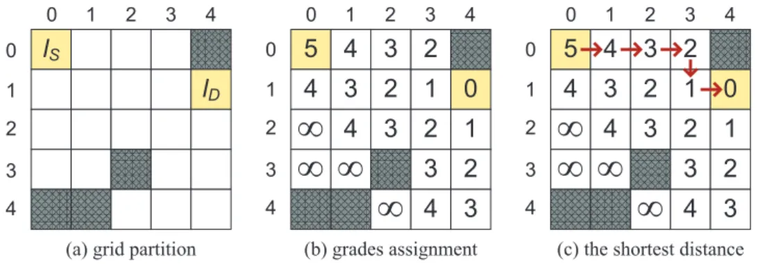
1. For each grid i that is not an obstacle, we associate it with a grade gi.
Initially gi = ∞ for all i.
2. We start from the grid with lD and set gD = 0. Then, for each adjacent
grid j (in the directions of north, south, east, and west) of a grid i that has already been assigned with a non-infinite grade, we set gj = gi+ 1.
If such a grid j is an obstacle, we just ignore it.
3. Repeat step 2 until the grid with lS has been assigned with a
4. We then start from the grid with lS. For the current grid i, we always
select the adjacent grid j that is not an obstacle and gj = gi − 1 as
the next grid to move toward. If two or more such grids are found, we select the one without changing the current moving direction. In the case that all candidates for the next grid will change the current moving direction, we randomly select one grid to move.
5. Repeat step 4 until we arrive at the grid with lD.
Fig. 3.1 gives an example, where the sensing field is modeled by a 5 × 5 grids. Two locations lS and lD are located at grids (0, 0) and (1, 4),
respec-tively. We start from the grid (1, 4) and assign a grade to each grid, until to the grid (0, 0), as shown by the numbers in Fig. 3.1(b). Then, we start from grid (0, 0) and find the shortest path to grid (1, 4) following the decreasing order of grades, as shown in Fig. 3.1(c). Note that when we arrive at grid (0, 1), there are two grids (0, 2) and (1, 1) that can be selected as candidates to move. Since the current moving direction is east (from (0, 0) to (0, 1)), we will select grid (0, 2) as the next grid because it need not to change the moving direction. The total moving time for a mobile sensor to move along this shortest distance is 5∆m+ 2∆t.
lS lD 5 4 4 3 4 3 2 3 2 1 2 3 4 0 1 2 3
(a) grid partition (b) grades assignment (c) the shortest distance 0 1 2 3 4 0 1 2 3 4 0 1 2 3 4 0 1 2 3 4 0 1 2 3 4 0 1 2 3 4 5 4 4 3 4 3 2 3 2 1 2 3 4 0 1 2 3
¥
¥ ¥
¥
¥
¥ ¥
¥
Figure 3.1: An example to calculate the shortest distance between two loca-tions lS and lD.
3.2
Finding a Suitable Hamilton Cycle
Recall that given a weighted complete graph G, our goal is to find a Hamilton cycle starting from l0 such that both Eqs. (3.1) and (3.2) can be satisfied. However, minimizing the total moving time of the mobile sensor (that is, to satisfy Eq. (3.1)) may not always guarantee that event locations with a higher priority can have a smaller waiting time (that is, to satisfy Eq. (3.2)), and vice versa. Therefore, we use a cost C to take care of the effects of both Eqs. (3.1) and (3.2):
C = f (v1) · w0,v1 + f (v2) · wv1,v2 + · · · + f (vn−1) · wvn−2,vn−1+ wvn−1,vn+ wvn,0,
(3.3) where f (·) ≥ 1. In particular, we should find a Hamilton cycle with a minimum cost C in step 4. Here, the cost should take both the total moving time and the priorities into consideration. Thus, we use a penalty function
f (·) to reflect the effect of priority. Intuitively, f (vi) should return a larger
value if an event location lvi with a lower priority is selected. By f (·), those
event locations with higher priorities could be selected first. However, to avoid the case that some nearer event locations are not selected due to their lower priorities, which may cause the mobile sensor to move in a too long distance, the returning value of f (·) cannot be too large. Therefore, we suggest setting the penalty function f (·) as follows:
f (vi) = 1 +
pvi− pmin
pmax− pmin
, (3.4)
where pmin = min
∀lj∈L−LV
{pj} and pmax = max
∀lj∈L−LV
{pj}, where LV is the set of
event locations that have already been visited. In Eq. (3.4), we can observe that when an event locations lvi with a larger value of pvi (i.e., lower priority)
is selected, the cost C will be increased since its corresponding weight wvi−1,vi
will increase. On the other hand, because 1 ≤ f (·) ≤ 2, the effect of penalty function will not be too significant. In this way, a nearer event location with lower priority could be selected to minimize the total moving time. Note that in Eq. (3.3), the term wvn−1,vn is not multiplied by the factor f (vn) because
lvn is the only candidate to be selected as the next visiting location.
It can be observed that finding a Hamilton cycle with a minimum cost C is NP-hard because we can reduce TSP to this problem by setting all f (·) = 1 in Eq. (3.3). Thus, we propose a heuristic solution by adopting a simple
greedy idea. Specifically, we start finding the cycle from the vertex l0. Given the current location li, we select an unvisited vertex lj as the next visiting
location such that the value of f (j) · wi,j can be minimized. We repeat the
above operation until all event locations are visited. With such a greedy selection, we can obtain a Hamilton cycle with a smaller cost.
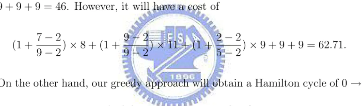
Fig. 3.2 gives an example to show how to find the Hamilton cycle with the minimum cost. By adopting the TSP solution, we will obtain a Hamilton cycle 0 → 7 → 9 → 2 → 5 → 0, which has a total edge weight of 8 + 11 + 9 + 9 + 9 = 46. However, it will have a cost of
(1 + 7 − 2 9 − 2) × 8 + (1 + 9 − 2 9 − 2) × 11 + (1 + 2 − 2 5 − 2) × 9 + 9 + 9 = 62.71. On the other hand, our greedy approach will obtain a Hamilton cycle of 0 → 2 → 5 → 7 → 9 → 0, which has a total edge weight of 9+9+8+11+12 = 49. This greedy approach will result in a cost of
(1 + 2 − 2 9 − 2) × 9 + (1 + 5 − 5 9 − 5) × 9 + (1 + 7 − 7 9 − 7) × 8 + 11 + 12 = 49. As can be seen, although our greedy approach will find a Hamilton cycle with a total edge weight larger than that of the TSP solution, it can result in a quite smaller cost. In this way, event locations with higher priorities can be visited first.
0
5
7
2
9
9
9
9
11
8
9
8
12
7
14
Figure 3.2: An example to show how to find the Hamilton cycle with the minimum cost.
3.3
Time Complexity Analysis
Next, we analyze the time complexity of our priority-based dispatch scheme. Let n be the number of event locations, and k be the number of grids in the sensing field, excluding those grids used to model obstacles. In step 1, conducting a full scanning takes O(k) time because the mobile sensor has to travel all grids. In steps 2 and 3, we need to calculate the shortest distance between any two locations. This operation takes O(k) time to assign grade to each grid and requires at most O(k) time to calculate the shortest path since the worst case is to pass through all grids. The above operation will be repeated ¡n+12 ¢ times. So, it takes totally ¡n+12 ¢· O(k) = O(n2· k) to conduct steps 2 and 3. Step 4 takes O(n) time due to the greedy selection, and step 5 requires at most O(k) time for the mobile sensor to visit all event locations (because the worst case is to travel all grids). Therefore, the total
time complexity of our priority-based dispatch scheme is
Chapter 4
Prototyping Experiences
We have implemented a prototyping system to monitor CO2 densities in an indoor environment. Such a prototyping system is consisted of a control server and a mobile sensor. The mobile sensor will be commanded to fully scan the environment to collect CO2 densities inside the room. Then, the control server will identify some locations with higher CO2 densities (that is, potential CO2 sources) and request the mobile sensor to visit these locations, according to our proposed greedy dispatching approach. Below, we give our prototyping experiences, including hardware specifications and the user interface at the control server.
4.1
Hardware Specifications
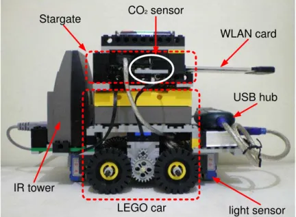
Fig. 4.1 shows our mobile sensor. It consists of following major compo-nents:
• Stargate processing board: The Stargate [25] is the major process-ing platform of the mobile sensor. It is composed of a 32-bits, 400-MHz Intel PXA-255 XScale RISC processor with 64 MB main memory and 32 MB extended flash memory. It also has a daughter board with an RS-232 serial port, a PCMCIA slot, a USB port, and a 51-pin exten-sion connector. It drives the CO2 sensor through a COM port, and an IEEE 802.11 WLAN card through its PCMCIA slot. The Stargate controls the LEGO car via a USB port connected to a LEGO infrared (IR) tower, as shown in Fig. 4.1.
• LEGO car: The LEGO car [26] supports mobility for the mobile sensor. It has an infrared ray receiver in the front to receive commands from the tower (which are passed from the Stargate processing board) and two motors on the bottom to drive wheels. It also has several light sensors for the navigation purpose, which will be described later. • CO2 sensor: The CO2sensor is used to collect the CO2densities inside
is a solid electrolyte CO2 sensor that provides miniaturization and low power consumption. It can detect a range of 350 to 5000 ppm of CO2 density.
• IEEE 802.11 WLAN card: The control server will pass commands (for example, full scanning command and dispatching command) to the mobile sensor via the IEEE 802.11 WLAN card. When collecting CO2 readings from the CO2 sensor, the mobile sensor can also report the data to the control server through the WLAN card.
Note that some more sophisticated sensing devices can be attached to the mobile sensor to increase its sensing capability. For example, we can attach a webcam on the mobile sensor so that it can take snapshot at the event locations to provide image information. The size of the mobile sensor is approximately 20 cm × 15 cm.
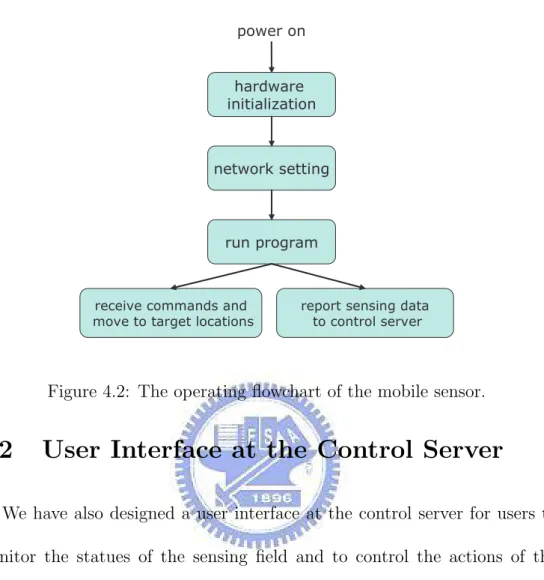
Fig. 4.2 gives the operating flowchart of the mobile sensor. Once powering on, the Stargate processing board will configure all corresponding hardwares, including the drivers of the IEEE 802.11 WLAN card, USB ports, and the COM port. Then, it will communicate with the control server to obtain a dynamic IP (this can be done by setting a DHCP server at the control server) and set up all necessary network configurations. After establishing the communication link with the control server, the Stargate processing board
IR tower
LEGO car light sensor WLAN card
USB hub Stargate CO2sensor
Figure 4.1: The mobile sensor.
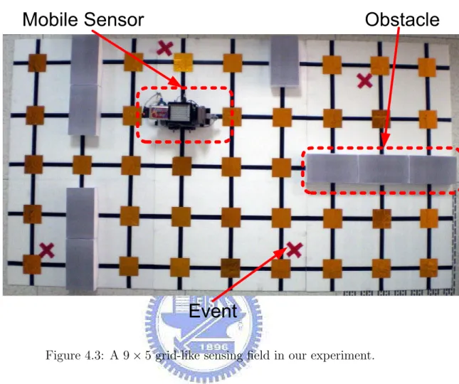
will notify the CO2 sensor to start collecting data and then wait commands from the control server (via the WLAN card). When receiving a dispatching command from the control server, the mobile sensor will move to the specified locations and report the CO2densities of these locations to the control server. In our prototyping, an experimental 9 × 5 grid-like sensing field is imple-mented, as shown in Fig. 4.3. Black tapes represent roads and golden tapes represent intersections. One mobile sensor is placed on the sensing field. We use some boxes to model obstacles. Red crosses on the sensing field indicate the event locations, where we can put some small piece of dry ice to simulate CO2 sources.
hardware initialization
network setting
run program power on
receive commands and move to target locations
report sensing data to control server
Figure 4.2: The operating flowchart of the mobile sensor.
4.2
User Interface at the Control Server
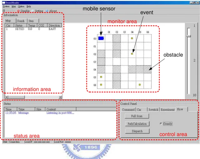
We have also designed a user interface at the control server for users to monitor the statues of the sensing field and to control the actions of the mobile sensor, as shown in Fig. 4.4. It has four areas: information, monitor, status, and control areas. The information area shows the current status of the mobile sensor, including the readings of the CO2 density, the location and direction of the mobile sensor, and so forth. The monitoring area illustrates the state of the sensing field, where the blue rectangle represents the mobile sensor, the small yellow rectangles indicate event locations, and the grids marked with oblique lines are obstacles. The status area gives the server’s status, including the contents of packets exchanged with the mobile sensor.
Figure 4.3: A 9 × 5 grid-like sensing field in our experiment.
Finally, the control area provides an interface for users to control the motion of the mobile sensors. Users can issue a high-level command such as taking full scanning of the sensing field, or a low-level command such as moving one-grid length or making a 90-degree turning.
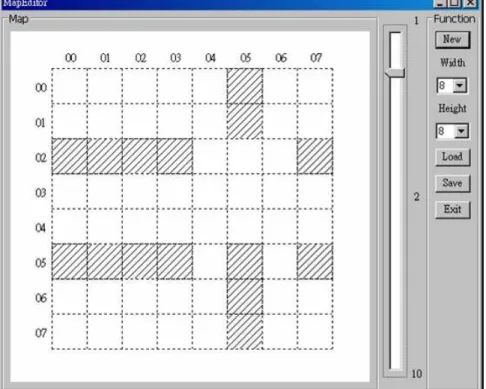
At the control server, we also set up a DHCP server to assign dynamic IPs to mobile sensors. Here, we use DHCPD32 [28] (version 1.10) as our DHCP server, as shown in Fig. 4.5. In addition, we also provide an interface for users to edit the map, as shown in Fig. 4.6. Users can specify the size of the
information area
status area control area
monitor area
mobile sensor
event
obstacle
Figure 4.4: User interface at the control server.
map, where the minimum and maximum map sizes are 2 × 2 and 100 × 100 grids, respectively. Obstacles can be specified by clicking corresponding grids. With this map editor, users can easily model the sensing field.
Fig. 4.7 shows some snapshots of the user interface when executing our priority-based dispatch scheme. Fig. 4.7 (a) illustrates the shortest path between two locations. Fig. 4.7 (b) gives the final cost matrix (with six locations), where the number in each grid indicates the length of the shortest
Figure 4.5: The DHCP server.
path between two locations. Fig. 4.7 (c) shows the basic motion operations of mobile sensor. For example, it takes four steps for the mobile sensor to move to the event location with priority 1. The mobile sensor should move to east with one grid-length, move to south with three grid-lengths, move to east with three grid-lengths, and finally move to north with three grid-lengths. Fig. 4.7 (d) shows the final result of the patrolling path of the mobile sensor.
(a) calculation of one path (b) the cost matrix
(c) the basic motion operations of the mobile sen-sor
(d) the patrolling path of the mobile sensor
Figure 4.7: Snapshots of the user interface when executing the priority-based dispatch scheme.
Chapter 5
Simulation Results
We also develop a simulator to evaluate the performances of the proposed dispatch scheme. We set up a sensing field as a 100 × 100 grids, on which there may be several obstacles. We randomly pick up 50, 100, 150, 200, 250, and 300 grids (excluding those grids representing obstacles) as event locations. The values of ∆m (that is, the cost to move one grid-length)
and ∆t (that is, the cost to make a 90-degree turning) are set to 1 and 2,
respectively. We mainly compare our priority-based dispatch scheme with the TSP approximate solution [16].
Fig. 5.1 shows the comparison of the total moving time of the mobile sensor under our priority-based dispatch scheme and the TSP approximate solution. We can observe that the TSP solution has a larger total moving time, because it is only an approximate solution. Our priority-based dispatch
scheme adopts a greedy approach, so that it can have a smaller total moving time. 900 1100 1300 1500 1700 1900 2100 2300 50 100 150 200 250 300 number of event locations
to ta l m o vi n g ti m e priority-based scheme TSP solution
Figure 5.1: Comparison on the total moving time of the mobile sensor.
Fig. 5.2 gives the comparison of the costs (by Eq. (3.3)) of the Hamilton cycles found by our dispatch scheme and the TSP solution. As can be seen, our priority-based dispatch scheme can find a Hamilton cycle with a cost smaller than that of the TSP solution. This indicates that event locations with higher priorities could be visited first.
Fig. 5.3 shows the waiting time of event locations, by adopting our priority-based dispatch scheme. In this experiment, we randomly select 100 locations as event locations. In Fig. 5.3, we can observe that event locations with higher priorities can have a shorter waiting time, which satisfy our goal.
1000 1500 2000 2500 3000 3500 4000 50 100 150 200 250 300 number of event locations
c
o
st
priority-based scheme TSP solution
0 200 400 600 800 1000 1200 0 20 40 60 80 100 priority w a it in g ti m e
(a) waiting time of each event location
0 200 400 600 800 1000 10% 20% 30% 40% 50% 60% 70% 80% 90% 100% priority a ve ra g e w a it in g ti m e
(b) average waiting time of each 10 event locations
Chapter 6
Conclusions
In this thesis, we have proposed a scenario to use mobile sensors to de-tect events in a region without any deployment of wireless sensor network. Mobile sensors will be first requested to conduct fully scanning of the region to collect rough information of the environment and to identify potential event locations. Then, mobile sensors will be dispatched to visit these event locations according to their priorities. We have proposed a priority-based dispatch scheme for mobile sensors to visit event locations. In particular, our dispatch scheme can reduce the total time for the mobile sensor to visit all event locations, while event locations with higher priorities can be vis-ited first. In this way, those event locations with higher priorities will suffer from lower waiting time. Simulation results have shown that our proposed dispatch scheme outperforms the approximated solution of TSP, on both the
total moving time of the mobile sensor and the average waiting time of event locations with higher priorities. In this thesis, we have also implemented a prototyping system to realize our dispatch idea. Such a prototyping sys-tem can be used to monitor CO2 densities in an indoor environment. The prototyping experience is also reported in this thesis.
Bibliography
[1] T. A. Dahlberg, A. Nasipuri, and C. Taylor, “Explorebots: a mobile net-work experimentation testbed,” in ACM SIGCOMM Workshop on Ex-perimental Approaches to Wireless Network Design and Analysis, 2005, pp. 76–81.
[2] D. Johnson, T. Stack, R. Fish, D. M. Flickinger, L. Stoller, R. Ricci, and J. Lepreau, “Mobile Emulab: a robotic wireless and sensor network testbed,” in IEEE INFOCOM, 2006.
[3] Y. C. Tseng, Y. C. Wang, K. Y. Cheng, and Y. Y. Hsieh, “iMouse: an integrated mobile surveillance and wireless sensor system,” IEEE Computer, vol. 40, no. 6, pp. 60–66, 2007.
[4] Y. Zou and K. Chakrabarty, “Sensor deployment and target localization based on virtual forces,” in IEEE INFOCOM, 2003, pp. 1293–1303.
[5] G. Wang, G. Cao, and T. L. Porta, “Movement-assisted sensor deploy-ment,” in IEEE INFOCOM, 2004, pp. 2469–2479.
[6] N. Heo and P. K. Varshney, “Energy-efficient deployment of intelligent mobile sensor networks,” IEEE Transactions on Systems, Man and Cy-bernetics - Part A: Systems and Humans, vol. 35, no. 1, pp. 78–92, 2005. [7] Y. C. Wang, C. C. Hu, and Y. C. Tseng, “Efficient placement and dispatch of sensors in a wireless sensor network,” IEEE Transactions on Mobile Computing, vol. 7, no. 2, pp. 262–274, 2008.
[8] G. Wang, G. Cao, T. L. Porta, and W. Zhang, “Sensor relocation in mobile sensor networks,” in IEEE INFOCOM, 2005, pp. 2302–2312. [9] P. Basu and J. Redi, “Movement control algorithms for realization of
fault-tolerant ad hoc robot networks,” IEEE Network, vol. 18, no. 4, pp. 36–44, 2004.
[10] Z. Butler and D. Rus, “Event-based motion control for mobile-sensor networks,” IEEE Pervasive Computing, vol. 2, no. 4, pp. 34–42, 2003. [11] M. Demirbas, A. Arora, and M. Gouda, “A pursuer-evader game for
sensor networks,” in Sixth Symposium on Self-Stabilizing Systems, 2003, pp. 1–16.
[12] C. Sharp, S. Schaffert, A. Woo, N. Sastry, C. Karlof, S. Sastry, and D. Culler, “Design and implementation of a sensor network system for vehicle tracking and autonomous interception,” in IEEE European Workshop on Wireless Sensor Networks, 2005, pp. 93–107.
[13] A. Verma, H. Sawant, and J. Tan, “Selection and navigation of mobile sensor nodes using a sensor network,” in IEEE International Conference on Pervasive Computing and Communications, 2005, pp. 41–50.
[14] Y. C. Wang, W. C. Peng, M. H. Chang, and Y. C. Tseng, “Exploring load-balance to dispatch mobile sensors in wireless sensor networks,” in IEEE International Conference on Computer Communications and Networks, 2007, pp. 669–674.
[15] M. Bellmore and G. L. Nemhauser, “The traveling salesman problem: A survey,” Operations Research, vol. 17, no. 3, pp. 538–557, 1968. [16] M. Blaser, “A new approximation algorithm for the asymmetric TSP
with triangle inequality,” in ACM-SIAM Symposium on Discrete Algo-rithms, 2003, pp. 638–645.
[17] Q. B. Zhu and S. Y. Chen, “A new ant evolution algorithm to resolve tsp problem,” in International Conference on Machine Learning and Applications, 2007, pp. 62–66.
[18] C. S. Jeong and M. Kim, “Fast parallel simulated annealing for traveling salesman problem,” Neural Network, vol. 3, pp. 947–953, 1990.
[19] A. Mohebifar, “New binary representation in genetic algorithms for solv-ing tsp by mappsolv-ing permutations to a list of ordered numbers,” in WSEAS International Conference on Computational Intelligence, Man-Machine Systems and Cybernetics, 2006, pp. 363–367.
[20] N. Yang, P. Li, and B. Mei, “An angle-based crossover tabu search for the traveling salesman problem,” in International Conference on Natural Computation, 2007, pp. 512–516.
[21] E. Baker, “An extra algorithm for time constrained traveling salesman problem,” Operations Research, vol. 31, pp. 938–945, 1983.
[22] X. S. Yan, A. M. Zhou, L. S. Kang, and Y. P. Chen, “Tsp problem based on dynamic environment,” in Intelligent Control and Automation Fifth World Congress, 2004, pp. 2271–2274.
[23] A. M. Campbell, “Aggregation for the probabilistic traveling salesman problem,” Computers & Operations Research, vol. 33, no. 9, pp. 2703– 2724, 2006.
[24] C. Y. Chang, H. R. Chang, C. C. Hsieh, and C. T. Chang, “OFRD: obstacle-free robot deployment algorithms for wireless sensor networks,”
in IEEE Wireless Communications and Networking Conference, 2007, pp. 4371–4376.
[25] Crossbow, “SPB400 - Stargate Gateway,” http://www.xbow.com.
[26] MINDSTORM, “Robotics Invention System,”
http://mindstorms.lego.com/eng/default.asp.
[27] TGS 4161, “The detection of Carbon Dioxide,”
http://www.tashika.co.jp.
[28] TFTPD32, “A free TFTP and DHCP server for windows, freeware TFTP server,” http://tftpd32.jounin.net.