行政院國家科學委員會專題研究計畫 成果報告
電子擴散系統的快速計算法(3/3)
計畫類別: 個別型計畫
計畫編號: NSC93-2115-M-002-004-
執行期間: 93 年 08 月 01 日至 94 年 07 月 31 日
執行單位: 國立臺灣大學數學系暨研究所
計畫主持人: 陳宜良
報告類型: 完整報告
報告附件: 出席國際會議研究心得報告及發表論文
處理方式: 本計畫可公開查詢
中 華 民 國 94 年 12 月 21 日
.
A NEW FORMULATION FOR CERTAIN INTERFACE PROBLEMS
IN POLAR COORDINATES AND APPLICATIONS∗
ZHILIN LI†, WEI-CHENG WANG‡, I-LIANG CHERN§, AND MING-CHIH LAI ¶
Abstract. In this paper, numerical methods are proposed for some interface problems in polar
or Cartesian coordinates. The new methods are based on a formulation that transforms the interface problem with a non-smooth or discontinuous solution to a problem with a smooth solution. The new formulation leads to a simple second order finite difference scheme for the partial differential equation and a new interpolation scheme for the normal derivative of the solution. In conjunction with the fast immersed interface method, a fast Poisson solver has been developed for the interface problems with piecewise constant but discontinuous coefficient using the new formulation in polar coordinates system.
Key words. interface problems, singular source, delta function, level set function, discontinuous
coefficients, polar coordinates, immersed interface method, smooth extension, fast Poisson solver.
AMS subject classifications. 65N06, 65N50
1. Introduction. Our original motivation of the paper is to solve certain elliptic interface problems defined in a disk using polar coordinates. To this purpose, we consider two types of interface problems.
1.1. Interface problem A. The Poisson equation with discontinuities and sin-gularities:
∆u(x) = f (x), x∈ R − Γ,
u(x) = u0(x), on ∂R, (1.1)
where ∆ is the Laplacian operator, R is a circular domain in two space dimensions,
∂R is the boundary of R, Γ ∈ C2 is a closed interface that does not pass the origin within the domainR. Across the interface Γ, the jump conditions in the solution and in the flux
[u]|X∈Γ = w(s), [un]|X∈Γ = v(s), w(s)∈ C2(Γ), v(s)∈ C2(Γ), (1.2) are prescribed, where s is the arc-length parameter of the interface Γ, un= ∂u∂n=∇u·n is the normal derivative of u, and n is the unit normal direction of Γ pointing outward, ∗The first author was supported in part by an ARO grant, 39676-MA, and an NSF grant, DMS-00-73403. The second author is supported in part by a NSC grant 89-2115-M-007-041 from Taiwan †Center for Research in Scientific Computation & Department of Mathematics, North Carolina State University, Raleigh, NC 27695. ([email protected].)
‡Department of Mathematics, National TsingHua University, Hsinchu, Taiwan, (wangwc @math.nthu.edu.tw)
§Department of Mathematics, National Taiwan University, Taipei, Taiwan, (chern @math.ntu.edu.tw)
¶Department of Applied Mathematics, National Chiao Tung University, Hsinchu 300, Taiwan, ([email protected])
see Fig. 1.1 for a geometric illustration. The jumps are defined as the difference of the limiting values from two different sides of the interface, for example
[u]|X∈Γ = lim
x→X,x∈R+u(x) −x→X,x∈Rlim −u(x)
define
= u+(X)− u−(X).
Across the interface, the source term f (x) can also have a discontinuity. We refer the readers to [9, 10, 11] for more explanations on the jump conditions. In this paper,
n τ r = rmax Γ R− β+ β− R+
Fig. 1.1. (a). A diagram of a circular domain R = R+∪ R−with an immersed interface Γ(s).
The coefficientsβ(x) may have a jump across the interface.
we use bold face of lower case letters such as x = (x, y), y,· · · to express points in the domainR, and bold face of upper case letters such as X, Y, · · · for points on the interface Γ unless stated otherwise. We use a Dirichlet boundary condition on ∂R for simplicity. Other boundary conditions can be treated using standard techniques.
1.2. Interface problem B. The elliptic equation with discontinuities and sin-gularities:
∇ · (β(x)∇u(x)) = f(x), x ∈ R − Γ,
u(x) = u0(x), on ∂R, (1.3)
where β(x) has a constant value in each sub-domain,
β(x) =
(
β+ if x∈ R+
β− if x∈ R−. (1.4)
The jump conditions
[u]|X∈Γ = w(s), [βun]|X∈Γ = v(s), (1.5) are prescribed along the interface Γ.
Note that the Problem A is a special case of Problem B with β− = β+ = 1. Problem B can be written as a single partial differential equation (PDE) to include the interface Γ in the domain in the sense of distribution. For example, if w≡ 0, then the problem (1.3)-(1.5) is well known to be equivalent to
∇ · (β(x)∇u(x)) = f(x) +
Z
Γv(s) δ2(x− X(s)) ds,
u(x) = u0(x), on ∂R,
(1.6)
where the equation is defined for all x∈ R including Γ, δ2(x) is the two dimensional Dirac delta function, see [10, 11] for the equivalence. The non-homogeneous jump in the solution can also be incorporated as a double layer source distribution along the interface Γ in the potential theory.
1.3. Some applications of the interface problems and a brief review of numerical methods. In the computation of micro-magnetics for ferromagnetic materials, or electrostatics for macromolecules, the potential function can be model as the solution of Interface problem A or B, see [5]. For a potential problems defined on an infinite domain, usually a big circle or rectangle is used to divide the infinite domain into two parts. If a circle is used in the separation, then the discussions in this paper can be applied.
Equation (1.6), in which the interface conditions (1.5) with w = 01 is expressed as a distribution using the Dirac Delta function, is the core of Peskin’s immersed
boundary (IB) method, see [18] for an overview. Numerically, the IB method uses a discrete delta function to distribute the integral in (1.6) to the nearby grid points.
The IB method have been used for many applications, particularly in fluid mechanics and mathematical biology. However, the IB method is known to be only first order accurate. In this paper, we will propose second order accurate algorithms for the interface problems A and B including the IB model (1.6), in polar coordinates.
The interface problems A and B probably can be solved with some efforts using other methods as well, for example, finite element methods with a body fitted grid; the first order (in the infinite norm) ghost fluid method (GFM) [15], which is simple to implement with a symmetric linear system of equations; the second order finite differ-ence methods based on integral equations [4, 16], the explicit jump immersed interface [21], and a few others. We refer the readers to [13] for a brief discussion of different methods. However, there are few discussions on how to apply these techniques to problems in polar coordinates.
The immersed interface method (IIM) [9, 11, 13] has a number of advantages in solving interface problems. However, the IIM method has not been directly applied to the Poisson equation in polar coordinates because the equation (1.3) has non-constant coefficients in polar coordinates. The jump relations of the solution and its derivatives are not as useful and informative in polar coordinates as the ones derived in [9, 11] for Cartesian coordinates.
1In some of the literature, Γ is called as an internal boundary, and (1.5) is called as internal
boundary conditions.
1.4. The contributions and the organization of the paper. In Section 2, a new formulation that is based on the extension of the jump conditions (1.2) along the normal lines is proposed. The new formulation transforms the interface problem A to a problem with a smooth solution. Theoretical analysis is given for the new formulation. In Section 3, a new numerical method that uses the new formulation introduced in Section 2 is proposed. The method is second order accurate in the maximum norm. The cost of the new method is about one call to a fast Poisson solver.
We should point out that the idea of extending the solution smoothly across the interface is not new, see, for example, the description of the IIM method in terms of extensions [3], the ghost fluid method [15] and maybe some others. The question is how to do it correctly and accurately to obtain efficient and accurate algorithm. Our proposed extension is particularly simple when the interface Γ is implicitly defined by a level set function. The strategy of the extension developed in this paper is unique and distinct from other approaches. The numerical method developed from the jump extension is simple and accurate for both the solution and the normal derivative.
In Section 4, we generalize the fast immersed interface method developed in [12] for the interface problem B in polar coordinates. The iterative method utilizes the new algorithm described in Section 3 as a fast Poisson solver. The iterative method for piecewise constant coefficient is second order accurate and the number of iterations is almost independent of the mesh size and the jump in the coefficient.
Numerical experiments and analysis are reported in Section 5.
2. A new formulation and extensions for the interface problem A. Let us repeat the interface problem A below:
∆u = f, x∈ R − Γ, [u]Γ= w(s). [un]Γ= v(s),
u(x) = u0(x). (2.1)
We assume that w∈ C2(Γ) and v∈ C2(Γ). Let ϕ(x) be a real valued function such that
ϕ(x) < 0, if x∈ R−, = 0, if x∈ Γ, > 0, if x∈ R+. (2.2)
We assume that ϕ(x) ∈ C3(R)2 in the neighborhood of the interface Γ, which is the zero level set ϕ(x) = 0. Usually, the level set function is chosen as the signed distance function from the interface, see [17, 20] and the references therein. In the neighborhood of the interface Γ, we define the extensions of w(X(s)) and v(X(s)) along the normal line (both directions) as
we(x) = we(X(s) + αn) = w(X(s)), (2.3)
2In the algorithms implementation, ϕ(x) just needs to be in C2(R), see Section 3-5. Second
and
ve(x) = ve(X(s) + αn) = v(X(s)), (2.4) for all α ∈ R such that the normal lines do not intersect, where n is the unit nor-mal direction pointing outward. We construct the following function based on the extension
˜
u(x) = we(x) + ve(x) ϕ(x)
|∇ϕ(x)|. (2.5)
Note that ˜u(x) ∈ C2 in the neighborhood of the interface Γ since we assume that
w(s), v(s), and Γ are all in C2. Define also
ˆ u(x) = H(ϕ(x))˜u(x) = 0, if ϕ(x) < 0, 1 2u(x),˜ if ϕ(x) = 0, ˜ u(x), if ϕ(x) > 0, (2.6)
in the same neighborhood in which ˜u(x) is well defined, where H(·) is the Heaviside function. We have the following theorem.
Theorem 2.1. Let u(x) be the solution of (2.1), ˆu(x) be defined in (2.6). Define
q(x) = u(x)− ˆu(x). Then in the neighborhood of the interface where we(x) and ve(x)
are well defined, the following are true:
∆q(x) = f (x)− H(ϕ(x)) ∆ˆu(x), x∈ R − Γ, (2.7)
[q]Γ = 0, [qτ]Γ= 0, [qn]Γ= 0, (2.8)
whereτ is the unit tangent direction, and qτ =∇q · τ = ∂∂qτ . In other words, the new
function q(x) is a smooth function across the interface Γ.
Proof: If x ∈ R−, then we have ˆu(x) = 0, so ∆ˆu(x) = 0, and H(ϕ(x)) = 0.
Therefore ∆q(x) = ∆u(x)−0 = f(x) and (2.7) is true. If x ∈ R+, then H(ϕ(x)) = 1, we have
∆q(x) = ∆u(x)− ∆ˆu(x) = f(x) − H(ϕ(x))∆ˆu(x).
What are left to prove are the jump conditions. Note that for any X(s)∈ Γ, we have [q]X(s)= [u]X(s)− [ˆu]X(s)= w(s)− ˜u+(X(s)) = w(s)− we(X(s)) = 0. Since w(s) is differentiable along the interface, so is we(X(s)). Differentiate the ex-pression above with respect to s, we get
d
ds[q]X(s)= w
0(s)− d
dswe(X(s)) = [qτ]X(s)= 0.
To prove the last jump condition, we proceed with the following derivation
∇ µ ve(x) ϕ(x) |∇ϕ(x)| ¶ · n = ve(x)∇ ϕ(x) |∇ϕ(x)|· n = ve(x) µ ∇ϕ(x) |∇ϕ(x)|+ ϕ(x)∇ 1 |∇ϕ(x)| ¶ · n, 5
here again we have used the fact that ve(x) is a constant along the normal line. Using the facts that n =∇ϕ/|∇ϕ|, ϕ = 0 on Γ, and ∇we(x)· n = 0, we conclude that
ˆ u+n(X(s)) =∇we(x)· n + ve(X(s)) ∇ϕ(X(s)) |∇ϕ(X(s))|· n = v(X(s)) ∇ϕ(X(s)) |∇ϕ(X(s))|· ϕ(X(s)) |∇ϕ(X(s))| = v(X(s)),
for any point X(s) on the interface. Therefore we get
[qn](X(s)) = [un](X(s))− ˆu+n(X(s)) = 0. 2
Remark: While q(x) is smooth across the interface Γ, its second derivatives usually have finite jumps across the interface. This can also be observed from equation (2.7) where the right hand side is discontinuous across the interface.
3. A numerical algorithm for the interface problems A. For a discontin-uous quantity such as u(x), f (x), etc., if x happens to be a grid point, then we define its value at the interface as the limiting value from a particular side of the interface, say theR+ side instead of the average of the limiting values from the two sides. This is because our algorithms actually approximate the partial differential equation from a particular side at the grid points near the interface.
In this section, we assume that β = 1 for simplicity. We describe our algorithm to solve (2.1). While the discussion is for polar coordinates, it can and have been applied to Cartesian grids with minor modifications.
We assume the domain is 0≤ r ≤ rmax, 0≤ θ < 2π. We construct the following grid in polar coordinates:
ri= µ
i−1
2 ¶
∆r, i = 1, 2,· · · , M with rM = rmax, ∆r = rmax
M−12;
(3.1)
θj = j∆θ, j = 0, 1,· · · , N − 1, with θ0= 0, ∆θ =2πN.
The j index ends at N − 1 because u(r, 0) = u(r, 2π). We choose ∆θ ∼ ∆r and introduce
h = max{ ∆r, ∆θ } (3.2)
for later use. We choose such a grid that the fast Poisson solver developed in [8] can be used. The level set function is defined at the grid points according to ϕij = ϕ(ri, θj). Because q(x) is smooth across the interface, we should be able to get reasonably good accuracy with the standard central five-point finite difference scheme. Clearly, the crucial part is how to extend w(s) and v(s) along the normal line accurately, and how far we should extend. These issues will be discussed in the following subsections.
We will use upper case letters such as U , Uij, Un, etc., for discrete approximations, and lower case letters such as u, q, ϕ etc., for the exact solutions or exact quantities unless stated otherwise.
3.1. The extension of the jumps along the normal line. Let
ϕmaxi,j = max{ϕi−1,j, ϕi,j, ϕi+1,j, ϕi,j−1, ϕi,j+1},
ϕmini,j = min{ϕi−1,j, ϕi,j, ϕi+1,j, ϕi,j−1, ϕi,j+1}.
(3.3) We define xij as an irregular grid point if
ϕmaxi,j ϕmini,j ≤ 0. (3.4)
We define xij = (ri, θj) as an sub-irregular grid point if it is not an irregular grid point, but one of its four neighbors is an irregular grid point.
If xij is neither an irregular nor a sub-irregular grid point, then we call it a
regular grid point.
Note that all the irregular and sub-irregular points are located within 2 grid size from the interface. In our numerical scheme, we only need to extend the jumps to all
the irregular and sub-irregular grid points. Given any such a grid point x = xij, the normal extension of the jumps is simply the jumps at the orthogonal projection of xij on the interface. So the crucial part is to find the projections effectively and accurately in the polar coordinates. Denote the projection of x = (r, θ) on the interface as X∗. Assuming that x is near the interface, we can write
X∗= x + αp, where p = ϕr(x) ϕθ(x) r2 . (3.5)
Using the Taylor expansion at x, we get the following quadratic equation for the unknown scalar α: ϕ(x) + (∇ϕ(x) · p) α +1 2 ¡ pTHe(ϕ(x)) p¢α2= 0, (3.6) where pTHe(ϕ) p = ϕ2rϕrr+ 2 r2ϕrϕθϕrθ+ 1 r4ϕ 2 rθϕθθ. (3.7)
In our algorithm, x is an irregular or sub-irregular grid point. The partial derivatives
∇ϕ(x), ϕrr, ϕrθ, and ϕθθare computed at the grid point using the standard centered five-point difference formula. For Cartesian coordinates, we refer the readers to [7, 14] for the details.
Remark: If (3.6) has more than one solution, which can happen only if the curvature is very large (O(h1)) relative to the grid, we just need to take one solution. The extension then is carried out with the chosen projection. This actually has little effect on the global accuracy because such points are few, if exist, see [2] for the reasoning of a similar problem.
3.2. An outline of the algorithm. Our algorithm for solving (2.1) is outlined below:
• Set-up a grid (3.1).
• Label all the grid points as regular, irregular, and sub-irregular.
• Find the projections for irregular and sub-irregular grid points using (3.5)
and (3.6).
• Extend the jumps to irregular and sub-irregular grid points from the
projec-tions to get ˜uij and ˆuij defined in (2.5) and (2.6).
• Form the discrete Laplacian
∆hUij= fij− H(ϕij)∆hu˜ij+ ∆huˆij+ Cij, if xij is irregular, fij, otherwise. (3.8)
where ∆h is the standard central finite difference operator. In polar coordi-nates, for example, it is
∆hUij= Ui−1,j− 2Uij+ Ui+1,j (∆r)2 + 1 ri Ui+1,j− Ui−1,j 2∆r + 1 r2i Ui,j−1− 2Uij+ Ui,j+1 (∆θ)2 .
• Apply the fast Poisson solver for polar coordinates [8] to solve the discrete
system of equations (3.8).
Now we can see why we just need to extend the jumps to the irregular and sub-irregular points. At a regular grid point where ϕij > 0, we have
−H(ϕij)∆hu˜ij+ ∆huˆij= ∆huˆij− ∆hu˜ij = ∆hu˜ij− ∆hu˜ij = 0.
If ϕij < 0, we have ∆huˆij = 0 and ∆hu˜ij = 0 from the definition. Therefore the term
−H(ϕij)∆hu˜ij+ ∆huˆij has no effect on the right hand side at regular grid points. Below we discuss how to determine Cij in (3.8) at irregular grid points. Define
Fij= fij− H(ϕij) ∆hu˜ij. (3.9) We expect Fij+ Cij to be a good approximation to ∆hqij = ∆h(uij− ˆuij). Without the correction term (i.e. Cij = 0), then the finite difference scheme (3.8) is first order accurate because the second order derivatives q(x) are discontinuous. The jumps in ∆q is reflected in the jump of Fij.
Let xij be an irregular grid point, the contribution to the correction term comes from those of the four neighboring grid points that are in the other side of the interface from the grid point xij. The correction term can be written as
Cij = X ik,jk H(−ϕi+ik,j+jkϕij) γi+ik,j+jk µ ϕi+ik,j+jk |∇ϕi+ik,j+jk| ¶2 F i+ik,j+jk− Fij 2 , (3.10)
where (ik, jk) ={ (−1, 0), (1, 0), (0, −1), (0, 1) }, H(·) once again is the Heaviside func-tion3, and γi+ik,j+jk are the coefficients of the discrete Laplacian ∆h corresponding
to Ui+ik,j+jk. In polar coordinates, these coefficients are γi±1,j = 1 (∆r)2 ± 1 2ri∆r, γi,j±1= 1 (∆θ)2. (3.11)
To show why we have the correction term (3.10), we introduce the following lemmas.
Lemma 3.1. Let q(x) = u(x) − ˆu(x), ∂2
∂n2 be the second order derivatives of q(x)
along the outer normal direction, F (x) = f (x)− H(ϕ)∆˜u(x). Then we have
·
∂2q ∂n2
¸
= [∆q] = [f− H(ϕ)∆˜u] = [F ] (3.12)
for any point on the interface Γ.
Proof: Since the Laplacian operator is invariant under orthogonal coordinates, we have ∆q = ∂ 2q ∂n2 + ∂2q ∂τ2 = F.
From [q] = 0, [qn] = 0, and [qτ] = 0 proved in Theorem 2.1, we can conclude that [∂∂τ2q2] = 0, which is derived in [9, 11] for the interface relations in the local coordinates. Therefore we conclude [∆q] = [F ] = · ∂2q ∂n2 ¸ . 2
The following lemma is the basis for the correction terms.
Lemma 3.2. Let ϕ(x) ∈ C3, xij be an irregular point with ϕij< 0 and ϕ
i+1,j > 0,
and ˜u(x) be well defined within two grid points from xij. Then we have
∆rhq(xij) define= q(xi−1,j)− 2q(xij) + q(xi+1,j)
∆r2 + 1 ri q(xi+1,j)− q(xi−1,j) 2∆r = ∂ 2q ∂r2(xij) + 1 ri ∂q ∂r(xij) + γi+1,j µ ϕi+1,j |∇ϕi+1,j| ¶2 Fi+1,j− Fij 2 (3.13)
Proof: Let X∗ be the projection of xi+1,j on the interface. Expanding ϕ(x) in Taylor expansion at X∗, we get
0 = ϕ(X∗) = ϕ(xi+1,j) +∇ϕ(xi+1,j)· (X∗− xi+1,j) + O ³
|xi+1,j− X∗|2 ´
.
Since x∗− xi+1,j is parallel to the normal direction n according to the definition of the projection, and ϕi+1,j> 0, we get
|xi+1,j− X∗| = |∇ϕ(xϕ(xi+1,j) i+1,j)|+ O ³ |xi+1,j− X∗|2 ´ (3.14) 9
which is known to be an approximate solution of the distance between X∗ and xi+1,j. Now we expand q(xi+1,j) in Taylor expansion at X∗ to get
q(xi+1,j) = q+(X∗) +∇q+(X∗)· (xi+1,j− X∗) +1 2(xi+1,j− X ∗)T He(q+(X∗)) (xi+1,j− X∗) + O ³ |xi+1,j− X∗|3 ´ ,
where He(q+(X∗)) is the Hessian matrix of q(x) at X∗. Since X∗− xi+1,j
|X∗− xi+1,j| =−n + O(|h2|),
and from the continuity condition of q(X∗) and its derivative, we get
q(xi+1,j) = q−(X∗)−∂q −(X∗) ∂n |xi+1,j− X ∗| +1 2|xi+1,j− X ∗|2∂2q−(X∗) ∂n2 +1 2|xi+1,j− X ∗|2 ·∂2q(X∗) ∂n2 ¸ + O(|xi+1,j− X∗|3).
Define the smooth extension of q−(x) fromR− intoR+ as
q−(xi+1,j) = q−(X∗)−∂q −(X∗) ∂n |xi+1,j− X ∗| +1 2|xi+1,j− X ∗|2∂2q−(X∗) ∂n2 . We have q(xi+1,j) = q−(xi+1,j) +1 2|xi+1,j− X ∗|2·∂2q(X∗) ∂n2 ¸ + O(|xi+1,j− X∗|3). Therefore ∆rhq(xij) =q(xi−1,j)− 2q(xij) + q(xi+1,j) ∆r2 + 1 ri q(xi+1,j)− q(xi−1,j) 2∆r =q(xi−1,j)− 2q(xij) + q −(x i+1,j) ∆r2 + 1 ri q−(xi+1,j)− q(xi−1,j) 2∆r + γi+1,j µ 1 2|xi+1,j− X ∗|2 ·∂2q(x∗) ∂n2 ¸ + O(|xi+1,j− X∗|3) ¶ .
Since q−(xi+1,j) is the extension of q−(x) from R− into R+, the expression above can be written as ∆rhq(xij) = ∂ 2q ∂r2(xij) + 1 ri ∂q ∂r(xij) + γi+1,j µ 1 2|xi+1,j− X ∗|2 ·∂2q(X∗) ∂n2 ¸ + O(|xi+1,j− X∗|3) ¶ . (3.15)
Finally from (3.14) and Lemma 3.1, we have 1 2|x − X ∗|2 ·∂2q(X∗) ∂n2 ¸ =1 2 µ ϕi+1,j |∇ϕi+1,j| ¶2 · ∂2q(X∗) ∂n2 ¸ + O(|xi+1,j− X∗|3) =1 2 µ ϕi+1,j |∇ϕi+1,j| ¶2 [F (X∗)] + O(|xi+1,j− X∗|3) =1 2 µ ϕi+1,j |∇ϕi+1,j| ¶2 (Fi+1,j− Fij) + O(|xi+1,j− X∗|3), where we have used (3.12), the fact that ϕi+1,j = O(|xi+1,j − X∗|), and [F (X∗)] = Fi+1,j− Fij+ O(|xi+1,j− X∗|). Plugging the expression above into (3.15),
we get the result of the lemma. 2
Lemma 3.2 tells us the contribution to the correction term from xi+1,j if it is in the different side of the interface from the grid point xij. Similarly, we can show the contributions to the correction term from the other neighboring points if they are in the different side of the interface from xij.
With the correction term Cij, we have matched the second order derivatives in the finite difference scheme. As a result, the computed solution of (3.8) has global second order accuracy in the infinite norm, see [13] for the analysis and Section 5 for the numerical results. If the extension is exact, the method described in this section gives exact solution when the solution is a piecewise quadratic function.
Since the left hand side of the finite difference equations (3.8) is the standard dis-crete Laplacian in polar coordinates, the FFT-based fast Poisson solver [8] or the one from Fishpack [1] can be applied directly. The main cost is the Poisson solver which typically requires M N log(M N ) operations. The cost to dealing with the interface is
O(N1) where N1is the total number of irregular and sub-irregular grid points. Usu-ally we have N1 ∼ max{M, N} which is one dimension lower than the total number of grid points.
3.3. Computing the normal derivative. Quite often, we need to compute not only the solution of the Poisson equation (2.1), but also the normal derivative of the solution at the interface. With the new formulation, it can be done easily since
q(x) is smooth across the interface.
Because the level set function is defined everywhere, or at least in a tube|ϕ(x)| ≤
δ, where δ is a given width, that contains the interface, we can naturally define the
‘normal derivative’ at all grid points in the tube as
∂u
∂n(x) =∇u(x) ·
∇ϕ(x)
|∇ϕ(x)|. (3.16)
Therefore we can get second order accurate ‘normal derivative’ at regular grid point in the tube using the central differencing. In this section, we discuss how to compute the normal derivative of the solution (2.1) at irregular grid points. This is one of the crucial steps in the applications of the level set method in which the velocity is
calculated at the grid points. The scheme discussed here will also be used in sub-section 4.4 to compute the normal derivative of the solution at the projections of irregular grid points on the interface.
Since we assume that the level set function be in C2(R), we can compute ∇ϕ/|∇ϕ| to second order accuracy using the centered differencing at all grid points. It remains to evaluate (ur, uθ) to second order accuracy. Again, we take advantage of the smooth property of q(x) with the following formula
∂Uij ∂r ≈ Ui+1,j− Ui−1,j 2∆r − ˆ
ui+1,j− ˆui−1,j
2∆r
+ H(ϕij)u˜i+1,j− ˜ui−1,j
2∆r + C r ij, if xij is irregular, Ui+1,j− Ui−1,j 2∆r , otherwise, (3.17) ∂Uij ∂θ ≈ Ui,j+1− Ui,j−1 2∆θ − ˆ
ui,j+1− ˆui,j−1
2∆θ
+H(ϕij)u˜i,j+1− ˜ui,j−1
2∆θ + C θ ij, if xij is irregular, Ui,j+1− Ui,j−1 2∆θ , otherwise, (3.18)
where the correction term is
Cijr = 1 2∆rH(−ϕi+1,jϕij) µ ϕi+1,j |∇ϕi+1,j| ¶2 Fi+1,j− Fij 2 − 1 2∆rH(−ϕi−1,jϕij) µ ϕi−1,j |∇ϕi−1,j| ¶2 Fi−1,j− Fij 2 , Cijθ = 1 2∆θH(−ϕi,j+1ϕij) µ ϕi,j+1 |∇ϕi,j+1| ¶2 Fi,j+1− Fij 2 − 1 2∆θH(−ϕi,j−1ϕij) µ ϕi,j−1 |∇ϕi,j−1| ¶2 F i,j−1− Fij 2 . (3.19) The correction terms are needed to offset the discontinuity in the second order deriva-tives of q(x). The reasoning is the same as discussed in sub-section 3.2.
4. The GMRES iteration for solving the interface problem B. In this section, we consider the algorithm for solving the elliptic interface problem (1.3)-(1.5) with β given by (1.4) (β+ 6= β−). Divided by the coefficient in each sub-domain of
R, the original problem can be written as
∆u = f β+ if x∈ R +, ∆u = f β− if x∈ R −, (4.1a) u(x, y) = u0(x, y), on ∂R, (4.1b)
excluding the interface Γ. This is a Poisson equation which can be solved easily using the algorithm discussed in the previous section if we know the jump in the solution [u] = w(s) and the jump in the normal derivative [un]. However, the usual jump condition is in the flux [βun] = v instead of [un]. We can not divide β from the flux jump condition because β is discontinuous. In [12], we proposed a fast iterative method for Cartesian grids. In this section, we describe a similar iterative method in polar coordinates for (4.1a) with jump condition (1.5) using the new fast Poisson solver and the new interpolation scheme described in Section 3.
As described in [12], the idea is to augment the unknown [un] = g(s) to the original problem to have the following system
∆u = f
β, if x∈ R
+∪ R−− Γ,
[u] = w(s), [βun] = v(s), [un] = g(s).
(4.2)
Note that g(s) is also an unknown. The system is still closed because of an additional equation [un] = g(s).
In the discretization, we represent the unknown jump g(s) = [un] only at the projections X∗k (k = 1, 2,· · · , NΓ) of the irregular grid points from the ϕ ≥ 0 side, where NΓis the number of such projections. We call these points as the control points. The reason to choose the projections on one particular side is to avoid clustered control points. The intermediate unknown jump g = [un] is defined at those control points as G = [G1, G2,· · · , GNΓ]
T in the discretization. The dimension of G is much smaller than that of the solution of U that is defined at all the grid points. Therefore we use the GMRES method [19] to find the discrete intermediate unknown G = [Un]. Once we know g(s), we can solve (4.1a) with [u] = w(s) and [un] = g(s) using the new method described in Section 3.
4.1. Setting-up the system of equations for [Un] and computing the residual. There are two coupled equations for the unknown u(x) and g(s). The first equation is the PDE ∆u = f (x)/β excluding the interface Γ with [u] = w(s) and [un] = g(s) are given. The solution depends on g(s) and can be written as ug(x). The second equation is the flux jump condition [β∂u∂ng] = v(s). So there are two steps discretizations:
• The system of the finite difference equations, which is obtained from the
algorithm discussed in Section 3 with given jumps [u] = w and [un] = g, can be written as (in the matrix-vector form)
AU + BG = F + Fw= F1, (4.3)
where U is the approximation to u(x) at all grid points, G is a discrete form of
g(s) at the control points on the interface, A is the matrix obtained from the
standard five point discrete Laplacian in polar coordinates, F is the vector formed from the source term; Fw is the part of−H(ϕij)∆hu˜ij+ ∆huˆij+ Cij in (3.8) corresponding to the jump [u] = w, and−BG is the part of the term corresponding to the jump [un] = g.
• The discretization of the flux jump condition [βun] = v in terms of u, [u] = w, and [un] = g using an interpolation scheme, can be written as
EU + DG = F2, (4.4)
where E, D, are two matrices. This is discussed in Section 4.4. If we put the two systems (4.3) and (4.4) together, we get
" A B E D # " U G # = " F1 F2 # . (4.5)
Since the dimension of G, which is defined at the control points on the interface, is much smaller than the dimension of U , which is defined at all grid points, it is advantageous to focus on the Schur complement
(D− EA−1B)G = F2− EA−1F1,
or SG = b, (4.6)
for the unknown G. The Schur complement system can be solved using the GMRES method [19]. Each iteration involves a call to the Poisson solver described in Section 3 to get U = A−1(F1− BG), and an interpolation scheme of (4.4) for the flux jump condition [βun] = v to get the residual vector
R(G) = (D− EA−1B)G−¡F2− EA−1F1¢= DG + EU− F2 (4.7) of the Schur complement system. In practice, the matrices A, B, E, and D, are not explicitly formed since the GMRES method only requires to compute the residuals.
Note that, if we take G = 0 in (4.7), then −R(0) = b is the right hand side of the Schur complement system. Also the residual vector (4.7) is the same as R(G) =
β+Un+(G)− β−Un−(G)− V , where Un±(G) is the vector whose components are the approximation of the normal derivative ∂u∂n±(X∗k), k = 1, 2,· · · , NΓ, at the control points.
4.2. An outline of the algorithm for solving the interface problem B.
• Set-up the grid (3.1).
• Label the grid points as regular, irregular, and sub-irregular. • Find the projections of irregular and sub-irregular grid points.
• Set [u] = w, [un] = 0, and solve the Poisson equation (4.1a)-(4.1b). Evaluate the residual (4.7) which gives the right hand side b for the equation (4.6).
• Set G0
k = v(X∗k), k = 1, 2,· · · , NΓ, at the control points as an initial guess of
G.
• Use the GMRES method to solve the system of (4.6) with some pre-conditioning
techniques.
There are several important implementation details that are addressed at the following subsections.
4.3. Interpolating G at projections that are not control points. In the GMRES iteration, the unknown G is the intermediate jump in the normal derivative defined only at the control points, that is, the projections of the irregular grid points where ϕ≥ 0. However, when we solve the Poisson problem (4.1a) and (4.1b) using the algorithm described in Section 3, we need to know the jumps at all the projections before extending them to all irregular and sub-irregular grid points. This is done through the weighted least square interpolation [12]. At a projection X∗k which is not a control point, we use
Gk=X p
γpGp, (4.8)
to get an approximation of [un](X∗k) from those [Un](X∗p) at the control points. The summation include 3∼ 6 projections from the ϕ ≥ 0 side within a circle:
kX∗
k− X∗pk2≤ ².
In our experiment, we choose ² to be 2h∼ 3h. The circle should enclose at least three control points to ensure second order accuracy. If there are more than six control points in the circle, then we choose the six of them that are closer to X∗k than the others in the circle. The coefficients γpare obtained from the un-determined coefficient method by expanding g(X∗p) along the interface, see Section 3.2 in [14] for the detailed description of the least square interpolation scheme to determine γp. Note that we have omitted the dependency of p on the index k for simplification of notations.
4.4. Computing the residual of the Schur complement. In the GMRES iteration, given a guess G, the matrix-vector multiplication involves two steps. The first step is to solve the Poisson equation (4.1a)-(4.1b) to get U (G). The second step is to compute the residual vector R(G) in (4.7) which is the same as β+Un+(G)−
β−Un−(G)− V . Therefore we need to compute Un+(Gk) and Un−(Gk) at those control points X∗k.
Once again, it is easier to evaluate Q±n(G) because q(x) is smooth, where Q±n(G) is the vector whose components are the approximation of the normal derivative∂q∂n±(X∗k),
k = 1, 2,· · · , NΓ, at the control points. Once we have Q±n(G), we can get Un±(G) us-ing the relation u(x) = q(x) + ˆu(x). We have already described how to evaluate
(Q±n)ij≈ qn(xij) at grid points in sub-section 3.3. Therefore we can use an interpo-lation scheme to get (Q±n)k, an approximation to qn±(X∗k), from the values at nearby grid points. Since qn+(X∗k) = qn−(X∗k), we can either use
(Q+n)k = X
ij
γijk (Q+n)ij, (4.9)
and set (Q−n)k= (Q+n)k, or use
(Q−n)k = X
ij
γijk (Q−n)ij, (4.10)
and set (Q+n)k = (Q−n)k. Due to the jumps in the second order derivatives q(x), the results obtained from (4.9) and (4.10) are slightly different. We will explain in the
next sub-section for the choice of the scheme. The summation is done through the grid points in a neighborhood of X∗k. We use the nine point stencil centered at the irregular grid point whose projection is X∗k for the interpolation. If ϕij < 0, then (Q+n)ij is regarded as the smooth extension (up to second order derivatives) of Q+n from the + side and can be computed using
(Q+n)ij = (Q−n)ij+ [F ]ij ϕij
|∇ϕij|. (4.11)
Similarly, we use
(Q−n)ij = (Q+n)ij+ [F ]ij |∇ϕϕij
ij| (4.12)
to extend the (Q−n)ij from the − side to an irregular grid point where ϕij > 0 if necessary. The discrete average jump [F ]ij is defined as
[F ]ij = X i+ik,j+jk H(−ϕi+ik,j+jkϕij) (Fi+ik,j+jk− Fij) X ik,jk H(−ϕi+ik,j+jkϕij) , (4.13)
where (ik, jk) ={ (−1, 0), (1, 0), (0, −1), (0, 1) }, as we used earlier in (3.10). Note that at an irregular grid point, the denominator can not be zero. Once we have computed
Q±n(X∗k), the normal derivative of the solution at X∗k is then determined from
(Un−)k= (Q−n)k, (Un+)k = (Q+n)k+ ˆun(X∗k). (4.14)
We use a second order interpolation scheme. The coefficients γijk are determined form the weighted least squares interpolation, see Section 4 in [12]. The linear system of equations for γkij is under-determined and is solved by a singular value decomposition (SVD) approach. One of the advantages of such interpolation is that the magnitude of the coefficients can not be very large regardless of the position of X∗k. The total CPU time spent in dealing with the interfaces usually is less than 5% of the total CPU time. The main cost is the time used for the Poisson solver in polar coordinates.
4.5. The preconditioning Strategy. The iterative method described above works for the interface problem B. But the number of iterations seems to grow linearly with the mesh size, see Table 5.3. We believe this is because the flux jump condition involves the normal derivative. Some pre-conditioning techniques are crucial to reduce the number of iterations. Note that we do not form the iteration matrix for the Schur complement system. Our strategy of the pre-conditioning is to enforce the flux jump condition during the iteration which seems to work well. The pre-conditioning
techniques that we have implemented are the following: If β+< β−: (Q+n)k= X ij γkij(Q−n)ij, (Un+)k= (Q+n)k+ ˆun(X∗k), (Un−)k= (Q−n)k = v(X ∗ k)− β+Gk β+− β− , If β+> β−: (Un−)k= (Q−n)k = X ij γkij(Q+n)ij, (Un+)k= v(X ∗ k)− β−Gk β+− β− ,
The second part of the pre-conditioning strategy is the same as in [12] to enforce the flux jump condition, but the first part, which is discussed in the previous sub-section, is new in this paper. The reasoning is simple, for example, if β− > β+, then it is likely that u− is flatter than u+ from the jump relation in the flux. Therefore u−and
q−n are likely to be more accurate than u+ and q+n.
The computational cost of the algorithm described in this section is O (N o.(M N log(M N ) + N1)), where N o. is the number of iterations of the GMRES method and N1 is the total
number of irregular and sub-irregular grid points. Generally, the extra time spent in dealing with the interface is less than 5% of the total CPU time. The main cost is the Poisson solver at each iteration.
5. Numerical Examples. We have done intensive tests on the methods dis-cussed in this paper. Most of experiments are done on Sun Ultra workstations. Our computer codes4have not been optimized and parallelized. However, all the numerical results confirm second order accuracy for the solution and the normal derivative from both sides of the interface in the infinity norm. The extra efforts spent on the inter-face is only a small portion of the total machine time if we compute the interpolation coefficients outside of the GMRES iteration.
In this section, we present our results for the interface
ϕ(r, θ) = r− (r0+ λ sin(ωθ)) , 0≤ r ≤ rmax, 0≤ θ < 2π, (5.1) with different parameters. Note that ϕ depends on both r and θ.
5.1. An example in which β is a constant. Since any constant β can be absorbed in the source term, we simply take β = 1. We present our results for the interface
ϕ(r, θ) = r− (0.5 + 0.1 sin(4θ + π)) , 0 ≤ r ≤ 1, 0 ≤ θ < 2π. (5.2) To check the order of accuracy, we use two non-linear functions:
u(r, θ) =
(
r4, if ϕ(r, θ) < 0,
r2sin θ, if ϕ(r, θ)≥ 0, (5.3)
4The code is available to public upon request.
as the exact solution. Note that the solution depends on both r and θ. The source term excluding the interface Γ is
f (r, θ) =
(
16 r2 if ϕ(r, θ) < 0,
3 sin θ if ϕ(r, θ) > 0. (5.4)
The Dirichlet boundary condition at rmax = 1, the jump in the solution and the normal derivative are computed from the exact solution at the projections where
ϕ≥ 0.
Table 5.1 lists the grid refinement analysis of the computed results. The error of the computed projections is defined as
Ep= max k |re(θ
∗
k)− rk∗| (5.5)
where (r∗k, θ∗k)’s, are computed projections of all irregular grid points, re(θ∗) is the exact interface relation given by re(θ) = 0.5+0.1 sin(4θ +π). The error in the solution
Eu is defined as
Eu= max
0≤ i ≤ M
0≤ j ≤ N
|u(ri, θj)− Uij| . (5.6) where Uij is the computed solution at the grid points.
The error for the normal derivatives are measured at two levels. Eun,g is the error
measured at all irregular grid points
Eun,g = max
(ri,θj) is irregular|un
(ri, θj)− (Un)ij| , (5.7) while Eun,Γ is the error measured at all the projections of irregular grid points
Eun,Γ= max (r∗ k,θk∗) ¯¯ ¯un(rk∗, θk∗)− (Un)(r∗ k,θ∗k) ¯¯ ¯ , (5.8) where (Un)ij, (Un)(r∗
k,θ∗k) are computed normal derivative at grid points and at the
projections respectively. At a projection, we compare both (Un+)(r∗
k,θ∗k)and (Un−)(r∗k,θ∗k)
with the exact normal derivatives from each side of the interface. The convergence order rE(M ) is defined as
rE(M ) =log(E(M )/E(2M ))
log 2 . (5.9)
We see that the computed projections are third order accurate, the computed so-lution, the normal derivative at grid points, the normal derivative at the projections are all second order accurate.
5.2. Numerical examples in which β is a piecewise constant. Now we consider the case where β is discontinuous. First we present the grid refinement analysis for the same exact solution as in the previous example. Therefore the solution is independent of β. Now we use a more complicated interface
ϕ(r, θ) = r− µ 1 2 + 1 5 sin(5θ) ¶ , 0≤ r ≤ 1, 0 ≤ θ < 2π, (5.10)
Table 5.1
Numerical results and convergence analysis for singular sources with N = 2M, β− =
β+= 1. M Ep rp Eun,g run,g Eun,Γ run,Γ Eu ru 40 1.915 10−4 1.294 10−2 9.044 10−3 1.877 10−3 80 2.452 10−5 2.97 3.053 10−3 2.08 2.071 10−3 2.13 3.384 10−4 2.47 160 3.079 10−6 2.99 6.147 10−4 2.31 5.262 10−4 1.98 7.427 10−5 2.19 320 3.866 10−7 2.99 1.595 10−4 1.95 1.476 10−4 1.83 1.786 10−5 2.06 640 4.834 10−8 3.00 3.768 10−5 2.08 3.759 10−5 1.97 4.245 10−6 2.07
see Fig. 5.1 (a). The source term now is
f (r, θ) =
(
16β−r2 if ϕ(r, θ) < 0,
3 β+ sin θ if ϕ(r, θ) > 0. (5.11) We normalize the PDE and the jump condition (1.3),(1.5) so that max{β−, β+} = 1
by dividing the larger β from the PDE (1.3) and the second jump condition in (1.5). Table 5.2
Numerical results and convergence analysis for discontinuous coefficient and singular sources withN = 2M. The solution is independent of the coefficient β.
(a) β−= 10−3, β+= 1. M Ep Eun,g run,g Eun,Γ run,Γ Eu ru N o. 40 3.828 10−3 0.1204 0.1746 4.099 10−2 10 80 4.565 10−4 3.147 10−2 1.94 4.857 10−2 1.85 9.972 10−3 2.04 8 160 8.954 10−5 4.292 10−3 2.87 1.815 10−2 1.42 1.551 10−3 2.69 8 320 1.035 10−5 1.448 10−3 1.58 2.503 10−3 2.86 2.628 10−4 2.56 5 640 1.247 10−6 1.716 10−4 3.08 5.608; 10−4 2.16 7.534 10−5 1.80 5 (b) β− = 1, β+= 10−3. M rp Eun,g run,g Eun,Γ run,Γ Eu ru N o. 40 10.77 12.59 3.150 22 80 3.1 2.5425 2.08 2.5425 2.21 0.6301 2.21 16 160 2.4 1.066 10−2 7.89 3.628 10−2 6.23 2.701 10−3 7.86 7 320 3.1 3.217 10−3 1.73 4.198 10−3 3.11 8.041 10−4 1.75 7 640 3.1 1.013 10−3 1.67 1.075 10−3 1.64 2.043 10−4 1.98 6
In Table 5.2, we present the grid refinement analysis with large jump in the coefficient β. The projection error is listed in the second column in Table 5.2 (a), while the convergence rate is listed in the second column in Table 5.2 (b). Again we see third order convergence. In Table 5.2 (a), the ratio of the β from different side of the interface is ρ = β−/β+ = 10−3. It is ρ = 103 in Table 5.2 (b). In either of
the case, we can see the average convergence rates for the rest of the quantities are quadratic. The number of iterations, or the number of calls to fast Poisson solver is small (less than 10). It is actually decreasing as the mesh size increases. It is almost the same for different ratio of β− and β+.
In Table 5.3, we present the grid refinement analysis with the solution dependent of the coefficient β u(r, θ) = r4 β−, if ϕ(r, θ) < 0 r2sin θ β+ , if ϕ(r, θ)≥ 0. (5.12)
The source term is also adjusted accordingly. In Table 5.3, we show the grid refinement analysis with two extreme ratios of β. The problem is harder because one of the solution that is divided by the smaller β has large magnitude. We still observe second order convergence for all the quantities. The number of GMRES iterations remains small compared to the size of the problems and the large jump in the coefficient.
Table 5.3
Numerical results and convergence analysis for discontinuous coefficient and singular sources withN = 2M for the solution that depends on β.
(a) β− = 10−3, β+ = 1. The last column is the number of iterations without the preconditioning strategy described in Section. 4.5.
M Eun,g run,g Eun,Γ run,Γ Eu ru N o. N o.np 40 5.118 10−2 3.118 10−2 6.444; 10−2 12 21 80 1.261 10−2 2.02 1.126 10−2 1.50 1.546 10−2 2.06 12 22 160 1.615 10−3 2.97 3.335 10−3 1.75 2.853 10−3 2.44 13 21 320 3.798 10−4 2.09 7.267 10−4 2.20 5.720 10−4 2.32 14 26 640 8.295 10−5 2.20 1.428 10−4 2.35 1.541 10−4 1.89 9 33 (b) β− = 1, β+= 10−3. M Eun,g run,g Eun,Γ run,Γ Eu ru N o. 40 1.934 10−2 1.373 10−1 1.772 10−3 27 80 8.445 10−3 1.20 4.316 10−2 1.67 2.635 10−4 2.75 18 160 2.172 10−3 1.96 1.853 10−2 1.22 7.565 10−5 1.80 22 320 7.661 10−4 1.50 1.895 10−3 3.29 2.374 10−5 1.67 19 640 1.612 10−4 2.25 5.740 10−4 1.72 4.654 10−6 2.35 22 In the last column of Table 5.3, we show the number of iterations of the iterative method without the pre-conditioning strategy described in Section 4.5. We see the number of iterations is almost doubled and is growing. The accuracy is nearly the same and there is not need to list it.
We also tested the convergence behavior when β+ is close to β−. The number of iterations is small. For example, when β+ = 1 and β− = 1.1 or vise versa, only four
iterations are needed. This is true for all the tested mesh sizes, M = 40, 80, 160, 320, and 640.
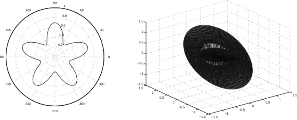
For interface problems, the errors may not decrease monotonically, see [12] for the analysis. Still, we see the average convergence rates for all quantities are quadratic. Usually, the more complex of the interface, the more oscillatory of the errors. In Table 5.4, we show the grid refinement analysis with a simpler interface (5.2). The other parameters are β− = 1, β+ = 10−2, and the exact solution is defined in (5.12) that depends on β. This test case is close to the tougher example in Table 5.3 (b). We see the grid refinement analysis behaviors more like a regular non-interface problem with the order of convergence approaches to number two more uniformly. Again the number of GMRES iterations is small and decreases a little as the size of the mesh increases. 0.2 0.4 0.6 0.8 1 30 210 60 240 90 270 120 300 150 330 180 0 −1.5 −1 −0.5 0 0.5 1 1.5 −1.5 −1 −0.5 0 0.5 1 1.5 −1.5 −1 −0.5 0 0.5 1 1.5
Fig. 5.1. (a) The domain r = 1 and the interface r = 0.5 + 0.2 sin(5θ) used in Table 5.2 and
Table 5.3. (b) The solution used for Table 5.1 and Table 5.2.
Table 5.4
Numerical results and convergence analysis for discontinuous coefficient and singular sources withN = 2M, β−= 1, and β+ = 10−2. The interface is defined in (5.2) which has smaller curvature than that of (5.10). The ratio in β, ρ = β−/β+ = 100 is also smaller
than that used in Table 5.2 and Table 5.3. As a result, the error behaviors more line a non-interface problem with a more uniform convergence rate.
M Eun,g run,Γ Eun,Γ run,Γ Eu ru No. 40 5.952 10−4 1.064 10−3 3.104 10−2 12 80 1.227 10−4 2.28 3.238 10−4 1.72 8.499 10−3 1.87 13 160 2.441 10−5 2.33 9.488 10−5 1.77 2.417 10−3 1.81 11 320 4.746 10−6 2.36 2.434 10−5 1.96 5.882 10−4 2.04 9 640 7.853 10−7 2.60 6.083 10−6 2.00 1.461 10−4 2.01 9 As a final test, we check the effect of the regularity of the level set function ϕ(x) on the accuracy of the computed solution. Theoretically, the second order accuracy is guaranteed if ϕ(x)∈ C3in the neighborhood of the zero level set varphi(x) = 0 which is the interface. In implementation, the level set function needs to be ϕ(x)∈ C2and
|∇ϕ(x)| 6= 0 near the interface. In experiment, we have found out that ϕ(x) ∈ C2is
enough for second order accuracy. If ϕ(x)∈ C1, the algorithm still works and seem to have super-linear convergence, see Table 5.5. Ideally, the level set function should be chosen as the signed distance function which satisfies|∇ϕ(x)| = 1. If a level set function is not the signed distance function, then a re-initialization technique can be applied to get the signed distance function while the interface is unchanged, see [6, 17, 20].
In the test, the level set function is chosen as
ϕ(r, θ) =
(
r− 0.5, if r < 0.5,
r− 0.5 + (r − 0.5)l, if r≥ 0.5 (5.13) where l≥ 1 is an integer. We see that ϕ(x) ∈ Cl−1 but not Cl. The interface is the circle r = 0.5.
The exact solution is given in (5.12). The other parameters are β− = 1, β+ = 10−2. This test case is close to the tougher example in Table 5.3 (b). We see that when l = 3, ϕ(x)∈ C2, we have second order convergence. When l = 2, ϕ(x)∈ C1, the algorithm still works with a super-liner convergence. The accuracy is affected by the computation of second order derivatives in ϕ(x). In all of cases, the number of iterations is small because the interface is simple. Still, the number of iterations is smaller when l = 3 than that when l = 2.
Table 5.5
Effect of the regularity ofϕ(x) on the fast iterative method for the interface problem B. The parameters areN = 2M, β−= 1, andβ+= 10−2. The interface is defined in (5.13). In the first three columns, l = 3 and ϕ(x) ∈ C2, we see clearly second order accuracy. In the last three columns,l = 2 and ϕ(x) ∈ C1 but not inC2, the accuracy is affected.
M Eu, l = 3 ru, l = 3 No. l = 3 Eu, l = 2 ru, l = 2 No. l = 2 40 4.4608 10−3 10 5.4403 10−3 10 80 1.0608 10−3 2.0721 9 1.7050 10−3 1.6739 10 160 2.5915 10−4 2.0333 8 5.5425 10−4 1.6212 9 320 6.4062 10−5 2.0162 6 1.9660 10−4 1.4952 9 640 1.5920 10−5 2.0087 5 7.7421 10−5 1.3445 8
6. Conclusion. In this paper, we have proposed a new formulation that trans-forms the certain interface problems with discontinuous/non-smooth solution to a problem with a smooth solution. A second order scheme for the PDE and an in-terpolation scheme for the normal derivative are developed and tested for interface problems in polar coordinates. The method is easier to implement for both polar and Cartesian coordinates. There is no need to differentiate the jumps along the interface and use the local coordinates as the original IIM does. Coupled with the fast IIM idea, we have also developed a second order fast iterative method for Poisson equa-tions with piecewise constant but discontinuous coefficient. The number of iteraequa-tions is almost independent of the mesh sizes and the jumps in the coefficient.
7. Acknowledgment. The first author would like to thank the National Center for Theoretical Sciences (NCTS) of Taiwan for their support during his visit there (May 8, 2001–June 8, 2001). We would also like to thank Dr. K. Ito of North Carolina State University for beneficial discussions.
REFERENCES
[1] J. Adams, P. Swarztrauber, and R. Sweet. Fishpack. http://www.netlib.org/fishpack/. [2] R. P. Beyer and R. J. LeVeque. Analysis of a one-dimensional model for the immersed boundary
method. SIAM J. Numer. Anal., 29:332–364, 1992.
[3] D. Calhoun. A Cartesian grid method for solving the streamfunction-vorticity equations in
irregular geometries. PhD thesis, University of Washington, 1999.
[4] H. W. Chen and L. Greengard. A method of images for the evaluation of electrostatic fields in systems of closely spaced conducting cylinders. SIAM J. Appl. Math., 58:122–141, 1998. [5] Weinan E. Selected problems in material science. World Mathematics 2000, Springer, in press. [6] T. Hou, Z. Li, S. Osher, and H. Zhao. A hybrid method for moving interface problems with
application to the Hele-Shaw flow. J. Comput. Phys., 134:236–252, 1997.
[7] K. Ito, K. Kunisch, and Z. Li. Level-set function approach to an inverse interface problem.
Inverse Problems, 17:1225–1242, 2001.
[8] M. Lai and W-C Wang. Fast direct solvers for poisson equation on 2d polar and spherical geometries. Numerical Methods for Partial Differential Equations, in press, 2000. [9] R. J. LeVeque and Z. Li. The immersed interface method for elliptic equations with
discontin-uous coefficients and singular sources. SIAM J. Numer. Anal., 31:1019–1044, 1994. [10] R. J. LeVeque and Z. Li. Immersed interface method for Stokes flow with elastic boundaries or
surface tension. SIAM J. Sci. Comput., 18:709–735, 1997.
[11] Z. Li. The Immersed Interface Method — A Numerical Approach for Partial Differential Equations with Interfaces. PhD thesis, University of Washington, 1994.
[12] Z. Li. A fast iterative algorithm for elliptic interface problems. SIAM J. Numer. Anal., 35:230– 254, 1998.
[13] Z. Li and K. Ito. Maximum principle preserving schemes for interface problems with discon-tinuous coefficients. SIAM J. Sci. Comput., 23:1225–1242, 2001.
[14] Z. Li, H. Zhao, and H. Gao. A numerical study of electro-migration voiding by evolving level set functions on a fixed cartesian grid. J. Comput. Phys., 152:281–304, 1999.
[15] X. Liu, R. Fedkiw, and M. Kang. A boundary condition capturing method for Poisson’s equation on irregular domain. J. Comput. Phys., 160:151–178, 2000.
[16] A. Mayo and A. Greenbaum. Fast parallel iterative solution of Poisson’s and the biharmonic equations on irregular regions. SIAM J. Sci. Stat. Comput., 13:101–118, 1992.
[17] S. Osher and R. Fedkiw. Level Set Methods and Dynamic Implicit Surfaces. Springer , New York, 2002.
[18] C. S. Peskin. The immersed boundary method. Acta Numerica, pages 1–39, 2002.
[19] Y. Saad. GMRES: A generalized minimal residual algorithm for solving nonsymmetric linear systems. SIAM J. Sci. Stat. Comput., 7:856–869, 1986.
[20] J. A. Sethian. Level Set Methods and Fast Marching methods. Cambridge University Press, 2nd edition,1999.
[21] A. Wiegmann and K. Bube. The immersed interface method for nonlinear differential equations with discontinuous coefficients and singular sources. SIAM J. Numer. Anal., 35:177–200, 1998.