Evaluation of the temporal effect to the peak tailing in flow injection analysis

www.elsevier.com / locate / chroma

Evaluation of the temporal effect to the peak tailing in flow

injection analysis

*

Su-Cheng Pai

Division of Marine Chemistry, Institute of Oceanography, National Taiwan University, P.O. Box 23-13, Taipei, Taiwan Received 7 September 2001; received in revised form 3 January 2002; accepted 8 January 2002

Abstract

The deformation of a flow injection analysis peak from a Gaussian shape has two components: spatial and temporal. The former is mainly attributed to the Poisseulie effect in the tubular flow, whereas the latter is related to the observing position (of a fixed detector) at which signal is measured. The combination of the two makes a skewed peak track on the recorder chart. Therefore, an observed peak may imply a substantial fraction of a ‘‘false’’ tail due to the effect of non-simultaneous detection. An expanding-Gaussian model is proposed to simulate the purely temporal effect, and the asymmetric factors were compared with that of the experimental peak shapes. In most cases the peak deformation occurring in flow injection analysis should be regarded as ‘‘temporal’’. The contribution of the spatial effects (Poisseulie profile and others) might not be as significant as it was thought previously.  2002 Elsevier Science B.V. All rights reserved.

Keywords: Peak tailing; Flow injection analysis; Temporal effect

1. Introduction tank-in-series model [4], the stochastic statistical

model [5], and the solutions of the partial differential Many chemical instruments give output signals as equations for mass transfer kinetics along a column peaks. In chromatography the peak is generally [6–8]. However, after a numerical comparison Gol-symmetrical or Gaussian-like, but for flow injection shan-Shirazi and Guiochon [9] concluded that all analysis (FIA) it is frequently skewed with a tail. chromatographic models can be approximated by a The tailing phenomenon, important for optimizing Gaussian profile even when the column efficiency is instrumental conditions, has drawn intensive atten- low. Although each model does give an asymmetri-tion since the technique was introduced in 1975 [1]. cal peak shape at the initial stage, the skewness is A question is raised: why is the FIA peak asymmetri- considered ‘‘insignificant’’, far from enough to jus-cal? One may seek assistance from existing chro- tify the observations commonly seen in FIA work. matographic theories as both techniques share very Further explanations become complex. The con-much the same physical principles [2]. Several cept of ‘‘non-linear isotherms’’ have been used in chromatographic models are helpful in this respect adsorption chromatography to derive non-symmetri-including the progressively calculated plate [3] or cal peaks [10], but it surely cannot be valid for FIA due to the lack of a stationary phase. Instead, the physical models derived from Fick’s Law [11–15],

*Tel.: 1886-2-2362-7358; fax: 1886-2-2363-2912.

E-mail address: scpai@ccms.ntu.edu.tw (S.-C. Pai). which is based on the physical dispersion–diffusion

0021-9673 / 02 / $ – see front matter  2002 Elsevier Science B.V. All rights reserved. P I I : S 0 0 2 1 - 9 6 7 3 ( 0 2 ) 0 0 0 4 6 - 8

272 S

behaviors of a tubular flow, have been more favored. Together with the friction effect against the tube wall, the resultant ‘‘Poisseulie’’ or the ‘‘parabolic velocity’’ profile has been generally adopted as the major source for the peak tailing in flow injection analysis, and the ‘‘bow-shape’’ diagram appears frequently in papers and textbooks [1,16].

1.1. The observer’s position

One important factor, the observer’s effect or the temporal effect, might have been overlooked by FIA analysts. When a shape-changing object passes through a fixed narrow-slit scanning camera, the observer will receive a distorted picture. It relates only to the observer’s standing point and the move-ment of that object, and not to the real appearance of

the object at a time. The deformation due to the Fig. 1. Diagrams illustrating the possible relationships between the mass profile (left) and recorded peak shape (right). (a)

non-simultaneous detection is spatially ‘‘false’’. An

Assuming that the mass distribution in the tubular channel is

‘‘observed peak shape’’ implies the ‘‘real peak

asymmetrical due to the Poisseulie effect, and that the pattern is

shape’’ plus ‘‘temporal deformation’’. The concept is _{unchanged during its passage through the detector at position D,} not novel in the chromatographic field. Back in the _{the recorder will give peak shape exactly like the mass distribution} 1950s, a continuous plate theory given by Gluec- peak. The deformation of peak is purely spatial. (b) Assuming the mass distribution is symmetrical throughout but the sample zone is

khauf [17] has already demonstrated that the peak

expanding while moving, the detector will record a steeper peak

shape can be distorted to have a tail even when the

front and a prolonged peak tail. The deformation of peak is purely

mass distribution in a column is Gaussian. A work- _{temporal. (c) In real situation the skewed peak image might} sheet practice of the Glueckauf’s model is included _{attribute to the combination of both.}

in a recent textbook by de Levie [18].

Misinterpretation might start from here: some FIA

analysts tend to use experimentally observed peak ‘‘spatial profile’’ and ‘‘temporal deformation’’. They shape to represent the mass-distribution pattern in the are separated on a hypothetical basis. In the former tubing, as they deemed the difference is negligible. case (Fig. 1a), the injected sample section moves Indeed, the mass distribution curve, based on a faster at the center axis than near the tube wall, length coordinate, can be converted to a time scale. leading to an asymmetric distribution pattern. If the For example, the mean residence time or peak pattern remains unchanged during its passage appearance time tp can be calculated from t 5p through a detector, a skewed shape is recorded. The

2

pr L /F (where r is the tube radius, L the length of image reflects a purely spatial pattern. In the latter the tubing, F the flow-rate) or t 5 L /u (u the flowp case (Fig. 1b), if the injected sample section has speed). This ‘‘converted’’ time coordinate, although already become a Gaussian-like pattern soon after having identical scaling to that on the ‘‘observer’s’’ leaving the injector, and it is still broadening with time coordinate, is still spatial in nature. Without time as it travels, the sensor encounters first a steeper making a distinction between the two may lead to front and then records a prolonged tail when the further confusion when dealing with the peak shape main peak passes over. The deformation of the problems. observed peak is purely temporal.

In a real situation, the skewness of a peak should refer to the combination of the two processes (see

2. Theoretical Fig. 1c). However, since one can always derive the

asymmetrical parabolic laminar flow by equations, A diagram (Fig. 1) is presented to distinguish the only the spatial effect has been emphasized by FIA

1 / 2

modelists. The temporal effect, sounds insignificant that this coefficient, in cm unit, is equivalent to and difficult to verify experimentally, has been the square root of the theoretical plate height H in_]] L

Œ

usually ignored. chromatography. It also equals 2D/u in Fick’s law where D is the diffusion coefficient and u the flow speed [23]. The purpose of using of m or later m inL t

2.1. Mathematical approach

this paper is to emphasize the ‘‘expanding’’ nature of the injected sample zone, just for the convenience of For laboratory applicants, the mathematical

ap-FIA readers.) proaches are of value if they can be simple enough to

be practiced on a computer spreadsheet (e.g., Excel).

2.3. Spatial distribution profile The most successful one would be the exponentially

modified Gaussian function (EMG) [19–22]. It is

Combining Eq. (1) and a standard Gaussian based on the fact that all complicated models

con-equation and letting the total peak area as A , aL

verge to a Gaussian function, and the degree of

symmetric concentration distribution pattern C(L ) at deformation decays exponentially with time. Thus,

a given time is generated and it can be plotted on the through a convolution process, an EMG curve is

L coordinate:

generated (in Gaussian form plus decay function).

2

L 2L

The EMG function can indeed produce significant _A p

L 2

S

D

]]]

C(L ) 5 ]]e m 2L (2)

asymmetric peak shape even at high theoretical plate Lœ p

mL

œ

numbers. Even though the physical meaning has

been questioned by some scientists [9], it has been _{where L is the position of peak summit (usually}

p

widely adopted as a reasonable approach in the _{refers to the position of the detector on the L} chromatography field [23]. _{coordinate). The curve generated by Eq. (2), noted as} the mass distribution curve, cannot be observed temporally by a single fixed detector. It could only 2.2. Conceptual approach

be seen if there were ‘‘many’’ detectors set along the channel to detect simultaneously.

A more simple approach is described in this work

It is very easy for one to think that Eq. (2) can be namely, the expanding-Gaussian function. It follows

converted into time scale, as t is proportional to the posture of the EMG function that the mass profile p

2

L (t 5 L /u), and s ~t ; A and m can be

trans-in a tubular channel is eventually Gaussian. Instead p p p t p L L

formed into temporal terms A and m corresponding-of converging an exponential function, the Gaussian t t

ly. Thus, it can be ‘‘mistakenly’’ expressed as: curve is ‘‘transformed’’ from a spatial axis to a

temporal axis. The skewness of the observed peak is _A t 2t_p 2

t 2

S

D

]]]

generated by the Gaussian curve itself, as it expands C(t) 5 ]]e m_tœ2t_p (3)

mt

œ

while it moves. Therefore, the present model is more

a ‘‘conceptual’’ one than a mathematical fitting. _{This Gaussian-type curve, although on a time} Only two basic equations are involved: a standard _{scale, does not reveal the recorder output, as what} Gaussian equation, and one describing the expanding _{the detector receives should be on a ‘‘sequential’’} of its standard deviation along the x-axis. In FIA, x _{time axis. Therefore the peak generated by Eq. (3)} can be the length L of the tubular channel or time t. _{does not exist and should not be plotted.}

According to previous theories, the

‘‘zone-broaden-ing’’ of a Gaussian profile can be defined as the _{2.4. Temporal convolution} expanding of the standard deviation s of the peak,L

which is proportional to the square root of the travel _{To project the non-existing image of Eq. (3) from}

2

distance L at a constant flow speed (or s ~L ):L _{a ‘‘simultaneous’’ time coordinate to a ‘‘real’’ time} ] _{coordinate is named the ‘‘temporal convolution’’.} Œ

s 5 mL L L (1)

Since the observation is made at a single point, one where m is defined here as an ‘‘expanding coeffi-L should consider the standard deviation of a peak (s )t

] ]

Œ

274 S

means that the observed curve is composed of many t and m , to be significant when t is small or m isp t p t

mass–curve segments at various time t. Thus, by large, and vice versa. replacing t as t in the square root terms, a ‘‘spatial-p

temporal projection-transformation equation’’, or 2.5. Temporal shift of peak summit simply the ‘‘temporally convoluted Gaussian’’

(TCG) is given: It is interesting to find that the position of the

*

temporally convoluted peak (note as t ) appearsp

t 2t_p 2

At 2

S D

p

]]] Œ

C(t) 5 ]e m_t 2t (4)

Œ

mt 2pt height to that of the spatial peak at tp but with a

*

‘‘very’’ slightly higher peak height at t . The smallp

The peak generated by this TCG equation is not _{temporal shift (t 2 t ) is related to m but indepen-*}

p p t

symmetrical, but it reveals the output on a recorder _{dent to A or t . The scale is ca. 0.5 s when m 51.0}

t p t

1 / 2

chart. The temporal deformation fraction of Eq.(4) _{s at a constant flow speed, 0.4 s when m 50.9}

t

1 / 2 1 / 2

from a Gaussian profile can be defined as the _{s , and 0.3 s when m 50.8 s . The expanding}

t

difference between Eqs. (3) and (4): _{coefficient m may vary from system to system. A}

t

quick estimation can be made experimentally by

t 2t_p 2 t 2t_p 2

At 2

S D

S

D

measuring the ‘‘observed’’ peak area A , height h,

]]] Œ ]]] TD(t) 5 _Œ]e mt 2t 2 ]]e mtœ2tp t mt 2pt mt

œ

œ

1 / 2

In most FIA cases m should be around 1 s . has three ‘‘crossing knots’’ on the t axis, one near the t

peak summit, and the rest two at each side of the

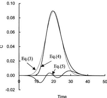
peak (Fig. 2). The skewness of a peak relates to both 2.6. Comparison to previous models

The TCG equation generates promising asymmet-ric peaks but with no surprise. This conceptual approach, without needing the knowledge of the theoretical plate number, physical diffusion–disper-sion or differential equations, leads to a resultant form almost the same as the famous Taylor–Aris series experiment [11,24], also as that derived by Lapidus and Amundson [6] for tubular chromatog-raphy. The skewed pattern generated is comparable to that by other sophisticated models as illustrated in the review paper by Golshan-Shirazi and Guiochon [9]. The TCG function is simpler than the EMG function, yet offers similar and reasonable skewed peak shapes.

The question becomes: is the zone broadening symmetrical at the very beginning and throughout, and the observed tail a ‘‘false’’ one due to the temporal effect? Or, is the zone broadening not

Fig. 2. The temporal deformation function, TD(t) (Eq. (5)) is the _{symmetrical initially, turning to be Gaussian but still} difference between a standard Gaussian curve (Eq. (3)) and the

viewed as having a temporal tail? Or, does the

TCG curve (Eq. (4)). Assuming m 51, A 5 1, and t 520, thet t p

asymmetric zone broadening accompany with the

curve crosses t-axis at t 515.8, 20.0 and 24.7. The temporal peak

temporal effect at all time? If both spatial and

*

(t 519.5, h 50.0898) appears slightly earlier than that expectedp

analysts would like to know: which is dominating in FIA?

3. Experimental

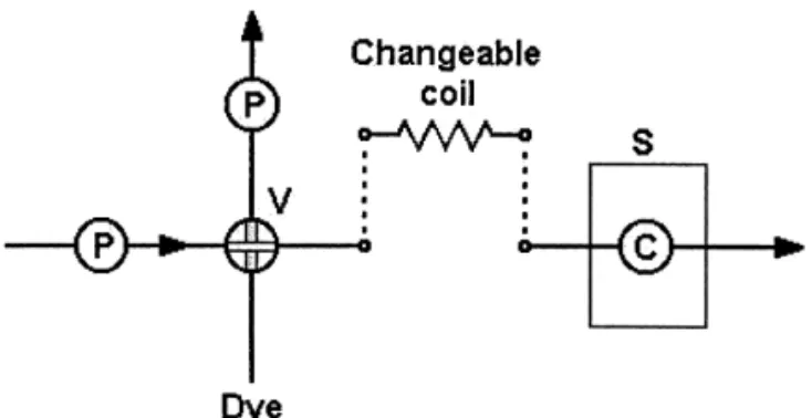
To further verify the temporal effect by experi-ment, a simplified flow injection system was assem-bled as shown in Fig. 3. It comprised a peristaltic pump running a distilled water carrier at a constant

Fig. 3. Layout of the flow injection system used in this study. The

rate of 4.25 ml / min; a Rheodyne four-way injector

delay coil is changeable from 0 to 360 cm long (made of PTFE

having an injection volume of 0.357 ml; a Hitachi

tube 0.8 mm I.D.). P, peristaltic pump; V, injection valve; S,

U-2000 double-beam spectrophotometer installed _{spectrophotometer; C, 1 cm flow cuvette (capacity 31 ml).} with a Hellma narrow-bore flow cuvette (light path

1.0 cm, capacity 31 ml); a delay coil that connected

*

regarded as t , whereas the ‘‘spatial’’ position tp p

between the injector and the detector. A series of

*

were retrieved by adding to tp a temporal shift of 0.5 delay coil of variable lengths (20–360 cm) was made

s. using PTFE tube of 0.8 mm I.D. wound onto a supporting rod. The coiled tubing facilitates mixing

4.2. TCG simulations in the flow channel [1].

A blue dye solution was used as the testing

By taking the experimental A , m , and corre-t t

sample; the undiluted absorbance reading was 0.805

sponding tp values (Table 1), and putting into the (at lmax5629 nm). Upon the injection of the dye

temporally convoluted Gaussian (TCG) equation, a solution (vol.50.357 ml), the recorder was pressed

series of peaks was generated (Fig. 6). The ‘‘on’’ to draw the peak track. Each resultant peak

asymmetry components (a and b) were obtained by was specified by measuring its peak appearance time

*

analyzing the TCG peak at 0.1h level (at t 2 a andp

*

(t ), peak height (h), and all those parameters usefulp

*

t 1 b). All simulated peak data are listed in Table 2.p

to characterize the peak asymmetry [25] (see Fig. 4), i.e., peak widths (W0.1 and W0.5) at 0.1h and 0.5h levels, respectively, components (a, b, c, d ) and their corresponding positions (t , t , t , t ).a b c d

4. Results and discussion

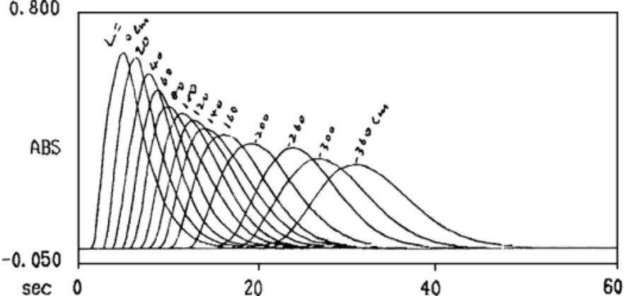
4.1. Experimental peaks

The recorded peak shapes (with delay coil lengths

L 50, 20, 40, 60, 80, 100, 120, 140, 160, 200, 260,

300, 360 cm, respectively) obtained by the proposed flow injection system are shown in Fig. 5. The peak information is listed in Table 1. The peak area was estimated to be 4.06 by taking the multiplied value of the initial bandwidth and absorbance of the injected sample. The expanding coefficient m wast

1 / 2

estimated from Eq. (6), to be 1.0160.037 s for Fig. 4. Parameters of an experimental asymmetrical peak. Asymmetry factor (A ) is defined by A 5 b /a.

276 S

Fig. 5. The peak tracks recorded by a Hitachi U-2000 spectrophotometer for a dye sample injected into the flow injection system with variable delay coil lengths. The injection volume was 0.357 ml. The lengths of delay coils were manually marked on the chart.

Table 1

Parameters taken from experimental peaks shown in Fig. 5

Coil length Peak height Peak position observed (s) Peak width Skewness m estimatedt Spatial

L (cm)c h (Abs) _{t t t t t W W a b A 5 b /a} by Eq. (6) tp a c p* d b 0.5 0.1 f 0 0.667 2.0 3.4 5.7 8.3 11.4 4.9 9.4 3.7 5.7 1.541 1.02 6.2 20 0.646 3.4 4.8 7.1 10.0 13.0 5.2 9.6 3.7 5.9 1.595 0.94 7.6 40 0.593 4.4 5.8 8.4 11.8 15.4 6.0 11.0 4.0 7.0 1.750 0.94 8.9 60 0.524 5.5 7.2 9.7 13.7 17.0 6.5 11.5 4.2 7.3 1.738 0.99 10.2 80 0.475 6.5 8.0 10.8 15.4 18.8 7.4 12.3 4.3 8.0 1.860 1.04 11.3 100 0.459 7.6 9.5 12.2 17.0 20.7 7.5 13.1 4.6 8.5 1.848 1.01 12.7 120 0.434 8.7 10.6 13.5 18.6 22.5 8.0 13.8 4.8 9.0 1.875 1.02 14.0 140 0.404 9.9 11.6 14.9 20.1 24.2 8.5 14.3 5.0 9.3 1.860 1.04 15.4 160 0.382 11.0 13.1 16.5 22.0 26.1 8.9 15.1 5.5 9.6 1.745 1.04 17.0 200 0.353 13.5 15.6 19.5 25.3 29.6 9.7 16.1 6.0 10.1 1.683 1.04 20.0 260 0.341 17.3 20.0 24.4 30.4 35.4 10.4 18.1 7.1 11.0 1.549 0.96 24.9 300 0.301 19.3 22.0 27.2 33.6 39.1 11.6 19.8 7.9 11.9 1.506 1.03 27.7 360 0.281 23.0 26.0 31.5 38.3 43.9 12.3 20.9 8.5 12.4 1.459 1.03 32.0

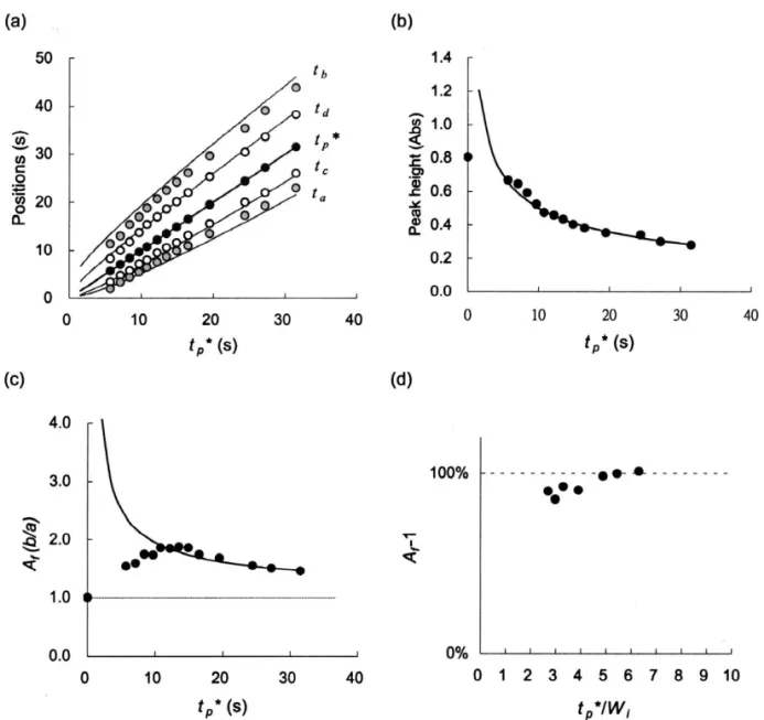
The resemblance of the simulated peak shapes (Fig. 6) to the experimental peaks (Fig. 5) is generally good. They all show characteristics (see Fig. 7) matching the basic FIA rules as stated in

˚ ˇ ˇ

textbook by Ruzicka and Hansen [1]: (1) the shape is

*

skewed when the mean residence time tp is short; and turns gradually to a more symmetrical-look

*

when tp is large; (2) the peak area remains the same at all times; (3) The peak height h decreases with

*

increase of the mean residence time t ; (4) the peakp

widths (W , W0.5 0.1 or a, b) increase with the square

Fig. 6. The observer’s FIA peaks generated by Eq. (4) assuming _{root of t . However, discrepancies are obvious when*}

p

A 54.06, m 51.01, and variable spatial peak positions (t 56.2–t t p _*

tp is very short, say, in the first 10 s in this work,

32 s, respectively, taken from Table 1). All curves were spatially

and they should be regarded as the ‘‘sample size’’

Gaussian before convoluted to the time coordinate. The

Table 2

Simulated peaks generated by Eq. (4) using A 5 4.06, m 5 1.01, and corresponding t values in Table 1 (also see Fig. 6)t t p Spatial Peak height Peak position calculated (s) Peak width Skewness

t (s)p h (Abs) _{t t t t t W W a b A 5 b /a} a c p* d b 0.5 0.1 f 6.2 0.657 2.48 3.58 5.70 9.17 13.38 5.59 10.90 3.22 7.68 2.385 7.6 0.592 3.32 4.64 7.10 10.92 15.38 6.28 12.06 3.78 8.28 2.190 8.9 0.545 4.15 5.67 8.40 12.50 17.18 6.83 13.03 4.25 8.78 2.066 10.2 0.508 5.00 6.71 9.70 14.06 18.95 7.35 13.95 4.70 9.25 1.968 11.3 0.483 5.75 7.60 10.80 15.38 20.42 7.78 14.67 5.05 9.62 1.905 12.7 0.455 6.72 8.76 12.20 17.02 22.25 8.26 15.53 5.48 10.05 1.834 14.0 0.433 7.66 9.85 13.50 18.54 23.94 8.69 16.28 5.84 10.44 1.788 15.4 0.412 8.65 11.02 14.90 20.15 25.75 9.13 17.10 6.25 10.85 1.736 17.0 0.392 9.83 12.38 16.50 22.00 27.78 9.62 17.95 6.67 11.28 1.691 20.0 0.361 12.07 14.96 19.50 25.42 31.53 10.46 19.46 7.43 12.03 1.619 24.9 0.323 15.86 19.24 24.40 30.95 37.56 11.71 21.70 8.54 13.16 1.541 27.7 0.306 18.07 21.71 27.20 34.08 40.95 12.37 22.88 9.13 13.75 1.506 32.0 0.285 21.53 25.54 31.50 38.85 46.10 13.31 24.57 9.97 14.60 1.464 *

Note that the appearance of the peak (t ) is 0.5 s earlier than the spatial t .p p

*

4.3. The sample size effect larger than 10 s (t /w . 2) to skip the sample sizep i

effect. Although the digitizing of the experimental It is common to use larger injection size in FIA peak widths might not be very precise, it does give (compared to chromatography) to avoid losing sen- clear trends as can be seen in Fig. 7. Both a and b sitivity. Therefore the injection volume cannot be components gradually merge with the theoretical

*

treated like a small plug. Instead, the sample section lines when tp is larger than 15 s. Within the range of should be regarded to have a histogram-shape at the 10–20 s the asymmetry factor (A 5 b /a) for thef

beginning; which gradually becomes a plateau, then experiment peak is slight larger than of the TCG

*

a peak shape when tp becomes large. Taking the simulation. Therefore, the temporal effect may not present case for instance, the injection volume was be, although dominant, the only one that controls the 0.357 ml, at a flow-rate of 4.25 ml / min it equals an peak tailing.

initial zone width (W ) of ca. 5 s on the time scale.i The contributions by the temporal effect have been Accordingly, the TCG function is derelict within estimated by taking (A 21) as a parameter (Fig. 7d).f

* *

10 s due to the large sample size. For example, the For peaks with tp between 15 and 20 s (t /W 5 3–p i

initial absorbance of the dye was 0.805; but the TCG 4), the temporal effect conveys a contribution of simulation gives infinite h when t is zero (Fig. 7b).p .90% for the experimental deformation, leaving less

*

Also, experimentally the initial width components a than 10% for other effects. When tp is above 25 s

*

and b were both 2.5 s, leading to an initial A 51,f (t /W . 5), the temporal contribution raises inp i

*

while the TCG gives infinite A at t 50 because thef p proportion to nearly 100%, but reduces in scale. initial band width is assumed zero (Fig. 7c). The

difference on the peak shapes in the first 10s (or

L ,20 cm) is also noticeable. Experimental peaksc 4.5. A general aspect for FIA peaks

are fatter at the middle, whereas simulated peaks

have much slender looks even though the bottom Based on the above verifications, a general aspect (W0.1) is wider. for the FIA peak shape development stands out and it

can be stated in four stages:

*

4.4. Comparison on asymmetry factor Stage1: At the initial stage or when tp is close to

*

the initial zone width W (t /W , 2 in the presenti p i

*

278 S

Fig. 7. Comparison of parameters estimated from the observed peaks (circles) and from that generated by TCG equation (lines). (a) Position

* * *

of t , t , t , t versus t ; (b) peak height versus t ; (c) asymmetric factor, A 5 b /a, versus t ; (d) temporal contribution (A 21) versusa b c d p p f p f

* t /W .p i

which gives a plateau-shape pattern and masks all it is still viewed to have a tail on the recorder chart. other effects. The temporal effect becomes the dominating reason

* *

Stage2: When tp is larger (e.g., t /W . 2 in thisp i for the peak deformation.

* *

work), the initial sample zone becomes a peak, Stage4: When tp is very large (say, t /W . 50),p i

appearing with an asymmetrical tail. Both spatial the asymmetry factor A converges to 1 and the peakf

(e.g., the sample size effect and the Poisseulie effect) appearance becomes a Gaussian curve. Neither the and temporal components may co-exist and co-re- spatial nor temporal effect is significant, the ob-sponsible for the peak skewness. served peak shape reveals almost the same pattern as

* *

Stage3: When t is even larger (t /W . 5 in thisp p i the mass profile.

work), the spatial effects fade gradually leading to a In FIA application, it is quite common to have an Gaussian-like distribution in the tubular channel, but injection size of 0.1–0.5 ml and a residence time of

30 s–2 min for a sample peak. If the manifold is Acknowledgements

*

operated at a flow-rate of 5 ml / min, the t /W ratiosp i

lay in a range between 5 and 50 (i.e., stage 3). With The author would like to thank K.M. Chen, Y.H. this in mind one may consider that most of the peak Li, G.T.F. Wong, K. Ronning, and two anonymous skewness observed for FIA should be regarded as reviewers for their kind and useful criticism of the

*

temporal. For chromatography the t /W is usuallyp i manuscript. very large ( .100), the temporal peak tailing can

only be observed for those leading peaks at near the void position.

References

˚ ˇ ˇ

[1] J. Ruzicka, E.H. Hansen, in: Flow Injection Analysis, 2nd ed, Wiley, New York, Chichester, Brisbane, Toronto, Singapore,

5. Conclusion 1988.

˚ ˇ ˇ

[2] J. Ruzicka, G.D. Christian, Analyst 115 (1990) 475. [3] L.C. Craig, J. Biol. Chem. 155 (1944) 519.

There are no contradictions between the proposed

[4] A.J.P. Martin, R.L.M. Synge, Biochem. J. 35 (1941) 1358.

TCG equation and existing theories for

chromatog-[5] J.C. Giddings, H. Eyring, J. Phys. Chem. 59 (1955) 416.

raphy and for FIA, as all lead to the same conclu- _{[6] L. Lapidus, N.L. Amundson, J. Phys. Chem. 56 (1952) 984.} sion: the peak is skewed when time is short and _{[7] G. Carta, Chem. Eng. Sci. 43 (1988) 2877.}

gradually turns to a Gaussian-like curve when the [8] J.B. Rosen, J. Chem. Phys. 20 (1952) 387.

[9] S. Golshan-Shirazi, G. Guiochon, in: F. Dondi, G. Guiochon

time is prolonged. The difference would be that the

(Eds.), Theoretical Advancement in Chromatography and

present work ‘‘emphasizes’’ the temporal effect,

Related Separation Technqiues, Kluwer, Dordrecht, Boston,

which transforms the mass distribution profile from a _{London, 1991.}

spatial axis to a sequential time axis and gives a _{[10] K. Robards, P.R. Haddad, P.E. Jackson, in: Principles and} twisted peak shape on the recorder. It provides clues Practice of Modern Chromatographic Methods, Academic Press, London, Boston, San Diego, New York, Toronto,

for those who are not familiar enough with physical

Sydney, Tokyo, 1994.

or mathematical skills to understand when and why

[11] G. Taylor, Proc. R. Soc. London, Ser. A 219 (1953) 186.

is the peak not symmetrical. _{[12] R. Tijssen, Anal. Chim. Acta 114 (1980) 71.}

The temporal effect exists universally in either _{[13] J.M. Reijn, W.E. van der Linden, H. Poppe, Anal. Chim.} FIA or chromatography. However, it seems that Acta 114 (1980) 105.

[14] J.T. Vanderslice, K.K. Stewart, A.G. Rosenfeld, D.J. Higgs,

many scientists of both fields have neglected this

Talanta 28 (1981) 11.

effect completely, leading to contradictions when

[15] S.H. Isaac, H. Soeber, L.H. Cristensen, J. Villadsen, Chem.

they need to explain ‘‘unexpected’’ peak tailings:

Eng. Sci. 47 (1992) 1591.

chromatographers tend to explain in a kinetic way, _{[16] D.A. Skoog, F.J. Holler, T.A. Nieman, in: Principles of} whereas FIA users tend to elucidate on the Poisseulie Instrumental Analysis, 5th ed, Saunders College Pub. / Har-court Brace College Publishers, Philadelphia / Orlando, 1998.

effect. This could have been arisen from the

recogni-[17] E. Glueckauf, Trans. Faraday Soc. 51 (1955) 34.

tion of the theoretical plate numbers. For example,

[18] R. de Levie, in: Principles of Quantitative Chemical

Analy-FIA may have apparent smaller plate numbers due to

sis, McGraw-Hill, International Editions, New York, 1997.

the lacking of stationary phase and faster flow-rate. _{[19] J.P. Foley, J.G. Dorsey, J. Chromatogr. Sci. 22 (1984) 40.} However, it should be borne in mind that the scaling [20] D. Hanggi, P. Carr, Anal. Chem. 57 (1985) 2394.

[21] J.P. Foley, J.G. Dorsey, Anal. Chem. 55 (1983) 730.

is artificially defined, therefore direct comparison on

[22] J.P. Foley, Anal. Chem. 59 (1987) 1984.

plate numbers might not be appropriate.

[23] D.C. Harris, in: Quantitative Chemical Analysis, 4th ed, W.H.

The use of ‘‘time’’ as a parameter to evaluate the

Freeman, San Francisco, CA, 1995.

zone broadening is deemed more practical. Any _{[24] R. Aris, Chem. Eng. Sci. 9 (1959) 266.}

disparity from the TCG curve could account for the [25] B.A. Bidingmeyer, F.V. Warren Jr., Anal. Chem. 56 (14)