演化式投資組合風險值評估：極值理論與GARCH模型

行政院國家科學委員會補助專題研究計畫

; 成 果 報 告

□期中進度報告

（計畫名稱）

演化式投資組合風險值評估：極值理論與

GARCH 模型

計畫類別：

;

個別型計畫 □ 整合型計畫

計畫編號：NSC 94-2416-H-151-003

執行期間：

2005 年 8 月 01 日至 2006 年 12 月 20 日

計畫主持人：林萍珍

共同主持人：

計畫參與人員： 江秉修、簡偉倫、李俊逸、游景安

成果報告類型(依經費核定清單規定繳交)：

;

精簡報告 □完整報告

本成果報告包括以下應繳交之附件：

□赴國外出差或研習心得報告一份

□赴大陸地區出差或研習心得報告一份

;

出席國際學術會議心得報告及發表之論文各一份

□國際合作研究計畫國外研究報告書一份

處理方式：除產學合作研究計畫、提升產業技術及人才培育研究計畫、

列管計畫及下列情形者外，得立即公開查詢

□涉及專利或其他智慧財產權，□一年

;

二年後可公開查詢

執行單位：國立高雄應用科技大學 金融系

中 華 民 國 95 年 12 月 20 日

演化式投資組合風險值評估：極值理論與

GARCH 模型

摘 要 在投資組合中，投資報酬率之厚尾現象與波動之特性，對於提升投資組合最佳化及風 險值的估計精確度，如何有效的掌握與控制，以期有更好的投資組合報酬及更低的風險。 本研究將運用遺傳演算法(Genetic Algorithm)來挑選投資組合，同時以極值理論(EVT)評估 挑選投資組合的風險值(VaR)。財務資料通常不是常態分配，大部份具有厚尾現象，極值理 論使用極限分配可有效捕捉財務資料的厚尾現象，較能專注於資料部的變化，精確估算風 險值。本研究探用超越門檻值法(Peak Over Threshold, POT)，避免在估計風險值時因忽略極 端值所表達的訊息而造成偏估的情形。由遺傳演算法的非線性運算特性所得的最適解，作 為取得最佳報酬率與最低風險值的投資組合之依據，再以極值理論所計算的風險值，做回 溯測試，若超過門檻值的次數越少，則代表風險越低，反之，風險愈高。而對於未來的實 驗結果，期望能對於投資組合之報酬率與風險值的波動能有效控管，避免低估風險，造成 重大損失。 關鍵字：遺傳演算法(GA)、一般化自我迴歸異質條件變異數(GARCH)、極端值理論( EVT) Abstract

Value-at-Risk (VaR) has become a popular risk measure since it was adopted by the Bank for International Settlements and US regulatory agencies in 1988. The VaR concept has also been further extended to the portfolio Value-at-Risk (PVaR) measure used for managing risks and returns under a multiple-asset portfolio. Precise prediction of PVaR provides better evaluation criteria in areas such as investment decision-making and risk management. The two issues concerned with portfolio risk are efficient set selection and volatility forecasting. Most of the statistical portfolio selection models are based on linear functions under specific assumptions. Due to the fat-tailed distribution in most real financial time-series data, extreme value theory (EVT) is powerful in determining the VaR of a portfolio by concentrating on estimating the shape of the fat-tailed probability distribution. However, using EVT to evaluate the portfolio’s volatility is very difficult, because each asset within the portfolio has its own distinct peak threshold value. This study introduces an evolutionary portfolio volatility forecasting model to optimize portfolios under their maximum expected returns subject to a risk constraint. We use a genetic algorithm (GA) to extract the best portfolio set and most suitable peak threshold in order to estimate the portfolio’s VaR by means of EVT.

Keywords: Portfolio Value-at-Risk, Genetic Algorithms, Extreme Value Theory, Peak Over

Threshold. Historical Simulation, Exponential Weighted Moving Average.

1.緒論

投資之不確定性(Uncertainty)及預期報酬率(Expected Return)是財務領域研究的主軸。 對於市場價格波動與報酬的不確定，風險的觀念因而形成。風險控管的主要目的便在於研 究這個不確定部份的特性，並加以確認衡量其可能的大小。鑑於「可能之最大損失金額」 資訊對於最佳化投資組合選取之風險控管之研究，「風險值(VaR)」之觀念因此產生。 應用最佳化技術選取股票投資組合，同時配合EVT 方法，估計其最適股票投資組合之 風險值，評估其最佳化股票投資組合的有效性(Availability)。因此，合理之 VaR 值量化模型 應以機率理論中最大順序統計量(Maximum Order Statistic)的觀點出發，並依據極端值理論 （Extreme Value Theory，EVT）建構出 VaR 之可能分配形態。去除不合理之常態分配假設，

並且可以精確地捕捉最佳化投資組合資產報酬之厚尾現象，進一步了解損失與發生機率間 的對應關係，而如何有效捕捉財務資產報酬分配之厚尾現象及波動的特性，掌握最佳化投 資組合資產報酬分配厚尾之現象是為本研究的主要動機。 本研究應用遺傳演算法所選取之最佳化投資組合資產，進行風險值估計之研究，，希 望能增進估計效率及降低估計偏誤，並有效捕捉最佳化投資組合資產之下方風險，來評估 依據遺傳演算法所選取之最佳化投資組合資產的風險特性。

2.文獻探討

本研究應用的主要技術是遺傳演算法與極值理論以最佳化投資組合之風險值最佳化， 以下將針對這兩個主題進行理論說明與文獻探討。

2.1 遺傳演算法

達爾文所提出的進化論是基因演算法的基礎，John Holland提出基因演算法用來解決數 學尋優的方法，其經過這些年來的發展John Holland 14(1975)提出，遺傳演算法其目的是以 嚴密且具體的科學方法來解釋自然界中「物競天擇，適者生存」的演化定理，並且將演化 的過程與機制由資訊軟體模擬出來。 遺傳演算法利用三種基本的運作機制，包括選擇(selection)、交配(crossover)、突變 (mutation)。透過此三個過程的演化，由母代產生新的子代，在每一代中較佳的個體將有較 高的機率，部份或全部保留給下一子代。然而，在染色體實施選擇、交配、突變操作之前， 必須先決定編碼及適應函數。廣為使用的編碼方式是二進位編碼(binary coding)。選擇運算 就是要選擇出交配複製的染色體，根據每個染色體的適應函數值高低，決定該染色體被選 擇的機率。交配運算提供族群中不同染色體，可經由隨機交配過程互換基因，以產生新的 子代。將交配後產生的子代，根據預設的突變機率進行突變，即位元反轉（0 變 1，1 變 0）， 突變的機制可能引進新的基因樣式，避免過早收斂(premature convergence)。 遺傳演算法在風險模型上的應用，陳嘉民 (2004) [4] 使用了傳統風險值模型-蒙地卡羅 模擬法(Monte-Carlo Simulation)及人工智慧方法遺傳演算法(Genetic Algorithm, GA)、倒傳遞 類神經網路(Back Propagation Network, BPN)及模糊理論(Fuzzy Logic Theory)，無論選取何 種人工智慧方式所模擬的風險值，其預測績效均優於傳統蒙地卡羅模擬法，在投資組合績 效分析方面遺傳演化類神經網路模型亦較佳。

2.2 極值理論

統計學上，某些參數只適合描述整個分配的一部分，並不適合對整個分配作估計，而 風險值主要在探討金融資產左尾極端分配的特性，故本研究以極值理論針對資產左尾分配 的特性加以探討；在探討極值理論前，先定義何謂風險值(VaR)。VaR係指在特定的信賴水 準下，衡量某一特定期間，因市場環境變動，使某一投資組合或部位所可能發生的最大損 失期望值Jorion (2000) [15]。VaR在估計波動性的方法中Engle (1982) [20]以考慮條件變異數 的ARCH(Autoregressive Conditional Hetero-Skedastic Model)家族模型來捕捉波動性的變 動，允許預期條件變異數作為過去殘差的函數，使變異數能隨時間而改變，突破過去對波

動性衡量的方法，之後Bollerslev (1987) [ 7] 改良ARCH模型，稱一般化自我迴歸異質條件 變異數模型 (Generalized Autoregressive Conditional Hetero-Skedastic Model, GARCH)，卻必 須負擔參數估計不穩定的潛在風險。

極值理論最早由Gumbel (1958) [11] 提出探討有關極值事件的隨機過程；極值分配的特 性在於尾部的分配函數與分配參數，可以從極端值與超過某一門檻值經過統計的處理過程 而被算出，其專注於處理分配的尾部的優點。雖然Fama (1965) [9] 發現金融商品資料的分

配為非常態分配，但直到1990 年初極值理論應用到財務領域才逐漸變得重要及廣為接受，

極值理論用於估計財務領域中金融商品報酬分配(Profit and Loss Distribution)的尾部部分， 用以計算VaR值；Jorion (2000) [15] 提到極值理論可以應用在時間序列的資料，通常時間序 列資料有自我相關的狀況，提議可以採用McNeil & Frey (2000) [18] 所提出的方法，結合 GARCH模型與極值理論計算VaR值；魏輝娥 (2003) [6] 以Hill (1975) [13] 提出的動差法估 計尾部參數給極值模型獲得較佳的結果，與本研究使用的GPD法估計尾部參數，實際上都 常被使用，但GPD模型在實證上較Hill提出的方法簡單；Hans (2004) [12] 使用傳統的極值 模型與結合GARCH的條件極值模型對股價作VaR值的估計，其結果顯示，加入條件的極值 模型在較高的信賴水準下，估計VaR的確有較佳的結果。根據以上的文獻分析，極值理論 可在財務資料非常態分配假設下，有效計算投資組合報酬分佈之厚尾現象與波動性。

3.研究方法

本研究針對演化式投資組合選擇及求算風險值作探討，以下分成「研究流程」、「遺傳 演算法」、「風險值模型及衡量方法」等三大點作說明。

3.1 研究流程

本研究流程以GA 為基礎架構，提出的六個流程如圖 3-1： (1) 由 GA 的內部運作機制，即：選擇、交配、突變，產生一組新的投資組合。抓取 投資組合中各家特定時段之報酬率。 (2) 將所得之資料以報酬率由小到大排序，再取其前 n%之報酬率，並令此 n%區段中 的最大值為門檻值，以取得觀察樣本X 數列。 (3) 將觀察樣本代入 GDP，再對所得的估計式取對數概似函數。透過最大概似估計法 求取其估計參數β與ξ的估計式，再透過牛頓法(Newton Method)計算參數β與ξ 的最佳近似值。 (4) 將最佳近似值β與ξ代入超越門檻值法之計算式，估計 VaR 值。 (5) 再以所得之 VaR 值，對所選取的投資組合進行加權平均值。之後再對最後計算出 之加權平均值取倒數後，交由遺傳演化法記錄與比較。 (6) 當遺傳演算法結束後，其產生的投資組合即為最佳投資組合。

由資料庫取得資料，以GA 選取 風險最小之最佳化投資組合 將β與ξ之值代入超越門檻值 法之VaR 方程式，求出 VaR 值 利用所得VaR 值，計算投資組 合之加權平均數，並計算其倒 產生最佳投資組合 設定門檻值，取出投資組 合中，超越門檻值的數值 以最大概似法，計算GDP 之 機率密度函數的β與ξ最佳 近似值 計算適應函數值 訓練流程 圖3-1 研究流程

3.2 投資組合理論及遺傳演算法

在自由市場，無論任何類型的價格，均存在一連續性波動，而形成這種波動的主要因 素，可能來自各方面，如政治、環境、市場機能、天災…等等，而如何在這些因素下，有 效的將資金分配在不同的資產上，如股票、期貨…等等的金融商品，建立最佳的投資組合， 進而取得較低的風險及較高的報酬，即為投資組合理論。 遺傳演算法是根據生物界的演化過程－基因染色體複製、交配及突變，藉由電腦模擬 此種演化系統，配合環境適應函數或方程式，來評估那些基因可以遺傳，那些基因須被淘 汰，以尋求最佳解。 在使用遺傳演算法之前，必須先設定其初始值，即染色體編碼與及適應函數的設計， 以下分別於3.2.1 與 3.2.2 說明：

3.2.1 染色體編碼方式

X1 Xn

0 1 0 1 1 0 0 1 … … … 每一個Xi 代表一個基因編號，i=1,2…..n 所組成的染色體，每一條染色體的長度為 n， Xi 是由 0 與 1 所組成的二位元(bit)字串，0 代表不選取該基因，1 代表選取該基因。假設被 欲取出投資組合的樣本有50 項，每一個 bit 代表一項資產的編號，即一個基因，每一個染 色體長度則為50 個 bits。

3.2.2 適應函數

適應函數對於不同的問題，會有不同的設定，每個問題均要設定一個足以衡量該問題 的適應函數，才能取得有意義的績效。而適應函數即為生物界中的生存環境，每一代的演 化會都會為了適應環境，而有不同的演化結果，若演化後世代越能符合適應函數的要求， 表示此新一代的個體越能適應環境，才可演化出更優良的子代。本研究之適應函數係以風 險最小為原則，其定義與計算方式之說明如 (1) 式。 F=1/VaRp (1) 其中F：代表適應函數。VaRp：投資組合風險值，由極值理論所計算之VaR 值，由個別資 產的風險值取算術平值，代表投資組合風險值。

3.3 極值理論(Extreme Value Theory，EVT)

本研究係以極值理論之超越門檻值法計算風險值，以特定的門檻水準，取得超越門檻

值的極端值，並藉由GDP 分配函數及解非線性方程式－牛頓法，求出β與ξ最佳近似值，

並將此二值代入由條件餘額分配函數所衍生之方程式，計算風險值。

3.3.1 超越門檻值法(Peak Over Threshold)

此法重點，在於考慮超過某一門檻值之資料，避免忽視這些資料在估計風險值時，造 成估計偏誤的影響，換句話說，超越門檻值法所重視的，是超越門檻的資料，而非對於整 體的資料進行評估。假設門檻值為u，R_n,_u =

{

r1,_u,r2,_u,...,r_n,_u

}

為超越門檻值的報酬率資料，共 有Nc筆，Fc(x)為其條件餘額分配函數(Conditional Excess Distribution Function, CEDF)。

u r x x u F u F r F u F u F x u F u r x u r P x F_u − = ∞ ≤ ≤ − − = − − + = > ≤ − = , 0 , ) ( 1 ) ( ) ( ) ( 1 ) ( ) ( ) | ( ) ( 其中，F(c)為報酬率小於門檻值的累積機率密度數，其值等於

(

T−N_u

)

/T，T 為全部的樣本 數，N_u為超越門檻值之樣本的數目。

而經由Pickands(1975)與 Balkema and de Haan(1974)定理可知，當門檻值越大， 會越 趨近於柏拉圖分配 (Pareto Distribution, PD)，由此可知： ) (x F_u ) ( , x G_βξ 0 ) ( ) ( sup lim _, 0 = − − ≤ ≤ ↑ _{x r u}Fu x G x u βξ

⎪ ⎪ ⎩ ⎪⎪ ⎨ ⎧ = − ≠ ⎟⎟ ⎠ ⎞ ⎜⎜ ⎝ ⎛ + − = − − 0 , 1 0 , 1 1 ) ( 1 , ξ ξ β ξ β ξ ξ β x e x x G

以β與ξ二參數所表達的方程式，即為一般化柏拉圖分配(Generalized Paredo Distribution, GPD)，β為規模參數，ξ為形狀參數(尾端指數)，ξ是決定尾端消失的速度。 將CEDF 整理如下： ) ( )) ( 1 )( ( ) ( )) ( 1 )( ( ) ( ) ( ) ( 1 ) ( ) ( ) ( u F u F x F r F u F x F u F r F u F u F r F x F u u u + − = − = − − − = 再將F(u)=

(

T −N_u

)

/T 、x=r−u、Fu(x)=Gβ,ξ(x)代入所得式子： ξ ξ ξ β ξ β ξ β ξ 1 1 1 1 1 1 1 1 1 1 ) ( − − − ⎟⎟ ⎠ ⎞ ⎜⎜ ⎝ ⎛ ₊ − − = − + ⎟⎟ ⎠ ⎞ ⎜⎜ ⎝ ⎛ ₊ − − = − + ⎟ ⎠ ⎞ ⎜ ⎝ ⎛ − − ⎥ ⎥ ⎥ ⎦ ⎤ ⎢ ⎢ ⎢ ⎣ ⎡ ⎟⎟ ⎠ ⎞ ⎜⎜ ⎝ ⎛ ₊ − − = u r T N T N u r T N T N T N T T N T u r r F u u u u u u 設定一機率值α，令F(r)=P(r≤u)=α，且r為欲估計之風險值VaRα，可得： ⎪⎭ ⎪ ⎬ ⎫ ⎪⎩ ⎪ ⎨ ⎧ − ⎥ ⎦ ⎤ ⎢ ⎣ ⎡ − + = − + = ⎥ ⎦ ⎤ ⎢ ⎣ ⎡ − ⎟⎟ ⎠ ⎞ ⎜⎜ ⎝ ⎛ − + = − ⎟⎟ ⎠ ⎞ ⎜⎜ ⎝ ⎛ ₊ − = − ⎟⎟ ⎠ ⎞ ⎜⎜ ⎝ ⎛ ₊ − − = ⎟⎟ ⎠ ⎞ ⎜⎜ ⎝ ⎛ − + − = − − − − − − 1 ) 1 ( 1 ) 1 ( 1 ) 1 ( 1 1 1 1 1 1 ) ( 1 1 1 1 ξ ξ ξ ξ ξ ξ ξ β β ξ β ξ β ξ β ξ β ξ a N T u VaR u VaR a N T u VaR a N T u VaR T N a u VaR T N a u r T N r F u u u u u u (2) VaR 即為所求之風險值。而β與ξ未知，因此以下再以最大概似估計法，求取βξ值，過 程將在3.3.2 加以說明。

3.3.2 最大概似估計法(Maximum Likelihood Estimation)

本研究使用最大概似估計法計算GPD分配，用超越門檻值法所選取的樣本，如X={x1,

(1) GPD 函 數 ： ξ ξ β

ξ

_β

1 ,

(

)

1

1

−

⎟⎟

⎠

⎞

⎜⎜

⎝

⎛

+

−

=

i i

x

x

G

_{， 求 其 機 率 密 度 函 數 ， 可 得 ：} 1 1 ,

1

1

)

(

− −

⎟⎟

⎠

⎞

⎜⎜

⎝

⎛

+

=

ξ ξ β i

_β

ξ

_β

i

x

x

g

_，以下令

g

_β,ξ

(

x

_i

)

=

f

(

x

_i

)

(2) 對 f(x_i)取概似函數，即 ⎥ ⎥ ⎥ ⎦ ⎤ ⎢ ⎢ ⎢ ⎣ ⎡ ⎟⎟ ⎠ ⎞ ⎜⎜ ⎝ ⎛ + × × ⎥ ⎥ ⎥ ⎦ ⎤ ⎢ ⎢ ⎢ ⎣ ⎡ ⎟⎟ ⎠ ⎞ ⎜⎜ ⎝ ⎛ + × ⎥ ⎥ ⎥ ⎦ ⎤ ⎢ ⎢ ⎢ ⎣ ⎡ ⎟⎟ ⎠ ⎞ ⎜⎜ ⎝ ⎛ + = … = − − − − − − 1 1 1 1 2 1 1 1 n 2 1 1 1 ... 1 1 1 1 ) f(x . ) )f(x f(x L ξ ξ ξ

β

ξ

β

β

ξ

β

β

ξ

β

n x x x 1 1 2 1

₁

_...

₁

1

1

− −

⎥

⎦

⎤

⎢

⎣

⎡

⎟⎟

⎠

⎞

⎜⎜

⎝

⎛

₊

⎟⎟

⎠

⎞

⎜⎜

⎝

⎛

₊

⎟⎟

⎠

⎞

⎜⎜

⎝

⎛

₊

⎟⎟

⎠

⎞

⎜⎜

⎝

⎛

=

ξ

β

ξ

β

ξ

β

ξ

β

n n

x

x

x

(3) 由第(2)步算得之公式較不易計算，因此對其取對數：

⎥

⎦

⎤

⎢

⎣

⎡

⎟⎟

⎠

⎞

⎜⎜

⎝

⎛

+

+

+

⎟⎟

⎠

⎞

⎜⎜

⎝

⎛

+

+

⎟⎟

⎠

⎞

⎜⎜

⎝

⎛

+

−

−

+

−

=

β

ξ

β

ξ

β

ξ

ξ

β

x

x

x

n

n

ln

(

1

1

)

ln

1

ln

1

...

ln

1

)

ln(

_l

1 2

∑

=

⎟⎟

⎠

⎞

⎜⎜

⎝

⎛

+

−

−

+

−

=

n i i

x

n

1

1

ln

)

1

1

(

ln

β

ξ

ξ

β

(4) 分別以β、ξ對所得的式子作徧微分，並令其等於 0：

0

1

1

)

ln(

)

,

(

1 1

⎟⎟

₊

=

⎠

⎞

⎜⎜

⎝

⎛

+

+

−

=

∂

∂

=

∑

= n i i i

x

x

n

f

ξ

β

β

ξ

ξ

β

β

ξ

β

l

0

1

1

1

ln

1

)

ln(

)

,

(

1 1 2 2

⎟⎟

₊

=

⎠

⎞

⎜⎜

⎝

⎛

−

−

+

⎟⎟

⎠

⎞

⎜⎜

⎝

⎛

+

=

∂

∂

=

∑

∑

= = n i i i n i i

x

x

x

f

ξ

β

ξ

β

ξ

ξ

ξ

ξ

β

l

(5) 由(5)式及(6)式組合，視為一個新的二維函數：

(

)

(

)

_{2 1} 2 1

,

,

×

⎥

⎦

⎤

⎢

⎣

⎡

=

ξ

β

ξ

β

f

f

F

₍₂₎ 為求得β與ξ的最佳近似值，以下將使用牛頓法解此非線性聯立方程式，其演算過程於 3.3.3 說明。

3.3.3 牛頓法(Newton Method)

由3.3.2 所取得概似函數之非線性聯立方程式後，再以牛頓法求其最佳近似值，流程如 下： (1) 對(2)式分別以β及ξ進行徧微分：

2 2 2 2 1 1 ×

⎥

⎥

⎥

⎥

⎦

⎤

⎢

⎢

⎢

⎢

⎣

⎡

∂

∂

∂

∂

∂

∂

∂

∂

=

′

ξ

β

ξ

β

f

f

f

f

F

(3) 其中：

(

)

(

∑

=

+

+

⎟⎟

⎠

⎞

⎜⎜

⎝

⎛

+

−

=

∂

∂

n i i i i

_x

x

x

n

f

1 2 2 2 1

1

₁

₂

β

ξ

βξ

β

ξ

ξ

β

β

)

(

)

∑

∑

= = ⎟⎟⎠ + ⎞ ⎜⎜ ⎝ ⎛ + + + − = ∂ ∂ n i _i i n i i i x x x x f 1 2 1 2 1 1 1 ₁

ξ

β

ξ

ξ

β

β

ξ

ξ

ξ

(

)

∑

∑

= = ⎟⎟⎠ + ⎞ ⎜⎜ ⎝ ⎛ ₊ + + − = ∂ ∂ n i _i i n i i i x x x x f 1 2 1 2 2 1 1 ₁ ξ β ξ ξ β β ξ ξ β

(

)

∑

∑

∑

= = = ⎟⎟⎠ + ⎞ ⎜⎜ ⎝ ⎛ + + + + ⎟⎟ ⎠ ⎞ ⎜⎜ ⎝ ⎛ + − = ∂ ∂ n i i n i i i n i i x x x x x f 1 2 2 1 2 1 3 2 2 _{ln 1} 2 1 ₁ ξ β ξ ξ β ξ β ξ ξ ξ (2) 所得之(3)式，即為牛頓法所用之 Jacobian 矩陣： 2 2 2 2 1 1 ×

⎥

⎥

⎥

⎥

⎦

⎤

⎢

⎢

⎢

⎢

⎣

⎡

∂

∂

∂

∂

∂

∂

∂

∂

=

′

=

ξ

β

ξ

β

f

f

f

f

F

J

(3) 分別給定β與ξ初始值；設定一 N 值，代表運算的最大次數；設定一 k 值，代表目前 為第k 次運算；設定一容許範圍 TOL，代表若超過這個容許值，則停止運算，並輸出最 後β與ξ的結果。演算法如下： (4) 將β與ξ代入(7)式<0>：可得 1 2 2 1 i ,

(x

)

F

×

⎥

⎦

⎤

⎢

⎣

⎡

=

f

f

ξ β (5) 將β與ξ代入 J(x)，其中J(x)=(∂f(x)/∂x)，可得： 2 2 2 2 1 1 ,

(

)

×

⎥

⎥

⎥

⎥

⎦

⎤

⎢

⎢

⎢

⎢

⎣

⎡

∂

∂

∂

∂

∂

∂

∂

∂

=

ξ

β

ξ

β

ξ β

_f

_f

f

f

x

J

_i (6) 第 k+1 次要代入的β與ξ值，等於： ( ) ( )

⎥

⎦

⎤

⎢

⎣

⎡

+

⎥

⎦

⎤

⎢

⎣

⎡

=

⎥

⎦

⎤

⎢

⎣

⎡

+ + k k k k k k

y

y

2 1 1 1

ξ

β

ξ

β

其中y 矩陣為Fβ,ξ(xi)與Jβ,ξ(xi)的反矩陣，相乘後的負數：

( ) ( )

(

)

[

1 1

]

1

(

( )1 ( )1

)

2 1

₌

₋

−

_,

− − −

_,

−

⎥

⎦

⎤

⎢

⎣

⎡

_{k k k k} k k

F

J

y

y

ξ

β

ξ

β

當y 矩陣產生後，即計算第 k+1 次的β與ξ值，也就是 ( ) ( )

⎥

⎦

⎤

⎢

⎣

⎡

+ + 1 1 k k

ξ

β

式。 (7) 計算 y 陣列的歐基里德值，如下：

( ) ( )

2 2 2 1k

y

k

y

y

=

+

，其中 ( ) ( ) ⎩ ⎨ ⎧ − = − = + + k k k k k k y y ξ ξ β β 1 2 1 1 _{，若 y} < _{TOL，則表示已超出容許範} 圍，可結束計算，而此時β及ξ值即為最佳近似值。 (8) k=k+1，代表進入下一次計算，依此重覆(4)~(7)步驟，若 k 值超過 N 值，則結束所有計 算.，此時β及ξ值即為最佳近似值。

4. 實證結果與分析

本研究係使用極值理論，並以超越門檻值法，作為取得極端值之條件，再以取得之極 端值估算最大可能損失，即風險值，並與歷史模擬法與加權移動平均法計算後，所得之風 險值，比較與本研究差異之所在。 本研究之資料來源，是透過時報資訊所提供之股價週報酬率，取其排序後，特定門檻 百分比下的最小數列，此數列即為極端值，再以計算後所得之風險值，與實際的報酬率比 較，觀察成功的機率。

4.1 資料來源說明

本研究的資料來源，採用時報資訊的資料庫，其資料庫提供台灣大盤的各大產業股的 股票週報酬率，由於各類股在上市的時間上有所不同，以及時報資訊資料庫，有部份缺少 資料的情形，因此為方便資料的計算與分析，我們將資料擷取的時間設為一致，擷取的範 圍由1987 年 1 月第 1 周，至 2004 年 12 月最後 1 週，對於資料缺少的部份，則以當週的前 5 週報酬率為範圍，取其平均值，填補缺少的週報酬率。經過處理後，所得公司數為 78 家， 每家的週報酬率共932 筆，共計 72696 筆。 為計算每家公司之風險值，我們以時間由遠至近排序，從中取出一段時間的資料，作 為樣本期間，並利用移動視窗(Moving Windows)的方式計算出此樣本期間的風險值，再與 此段期間後的下一筆報酬率比較，而移動視窗的觀念，在於其移動後，資料會被更新，但 取出的筆數不變，也就樣本期間的筆數是固定不變的，最舊的資料會被剔除，最新的資料 會加入到最後一筆，其目的是為了讓實驗的過程更為客觀，圖4-1 為實驗資料處理說明。

圖4-1 移動視窗

4.2 回溯測試

無論何種產業的企業，都希望能夠永續經營，除了提高知名度，及持續的獲利外，對 於風險的評估也是企業所必須執行的政策，而對於如何評估風險，企業常以風險值(VaR) 作為評估風險的基礎，準確的估算風險值，可以讓企業及早做好準備，以盡可能的避免破 產，但是風險值要如何估算才有其準確性呢？國際清算銀行(Bank of International Settlement, BIS)在 1996 年所頒行的巴塞爾資本協定(Basle Capital Accord, BCA)，其中提出對於風險值 的估算，建議應以回溯測試來驗證其準確性，以判斷風險值是否能有效滿足市場的實際情 況。計算方式是用過去一段時間的市場真實歷史資料，估算其風險值，再觀察實際市場損 失超越風險值的次數，亦即觀察其成功或失敗次數，以及成功率與信賴水準趨近的程度。 以BCA 所提到對於風險值的估計方式為基礎，我們從過去歷史實際市場損益中，取出 一段時間的樣本，其中N 筆為樣本期間，樣本期間總數為 N 筆，固定不變，而 M 筆則為 測試期間，因此樣本總數為N+M 筆，從 N 筆歷史損益計算出 VaR 後，再與第 N + i 筆實際 損益比較，若當日實際損益小於估算出的VaR 值，則表示成功，在所有樣本測試完成後， 將成功次數除以測試次數可得成功率(Ps)，即成功率(Ps) = 成功次數 / 測試期間，若成功 率大於信賴水準，表示估計之風險值有高估的現象，可能產生資金運用效率較低的情況， 反之，若成功率小於信賴水準，則表示估計之風險值有低估的現象，可能會使得企業發生 破產危機，雖然高估風險值會產生浪費資金的情況，但是低估卻會造成企業面臨破產危機。

4.3 實驗設計

本研究係以遺傳演算法之最適理論，與極值理論以極端值計算風險值的做法，估算每

組投資組合之最大可能損失。對於極端值的選取方式，本研究是以超越門檻值法(POT)，來 找出最適合估算的極端值及其個數，以下說明本研究如何取得極端值： 1. 從每支股票以特定期間選取的歷史報酬率樣本中，以時間為序列，選取適當 的數目作為樣本期間，其餘為測試期間，且樣本期間筆數>測試期間筆數。 2. 再將所選取之樣本期間，由小至大排序，以 n%作為取出極端值筆數的門檻 ，即門檻百分比。 3. 在不同的信賴水準下，均各有 1% ~15% 的門檻百分比，因此取出的極端值 數目也不同，由此估算不同的門檻百分比，所得到的風險值。 遺傳演算法是以使用者修改後的Fitness 函數，計算一代中每條染色體的 Fitness 值，做 為判斷是否可以讓染色體遺傳給下一代的依據，因此本研究將每一條染色體，視為一組投 資組合，而每一支股票均佔5 個 bit，第一個 bit 表是否有選取此支股票，其餘四個 bit 是用

以計算門檻百分比，但若門檻百分比為0，則此支股票即不選取，再以門檻百分比與樣本 期間相乘，可得極端值之筆數，而相乘之前即對樣本期間由小至大排序，此因本研究是以 最大可能的損失為目的，計算風險值，而排序後之樣本期間，負數均會集中在最前面，易 於將損失的極端值取出，取出極端值後，再代入牛頓法，計算GPD 函數中的β與ξ，再將 β與ξ，以及門檻百分比指定的門檻值，代入公式估算風險值，其後再將估算出之風險值 與樣本期間的下一筆報酬率，也就是與測試期間的報酬率比較，若風險值小於實際報酬率， 則表示成功，待所有測試完成後，再計算此支股票的平均成功率，在投資組合中選取到的 股票均依此類推，最後估算出來的投資組合平均成功率，即為此投資組合，也就是此條染 色體的Fitness 值，而每代每條染色體都依此 Fitness 值決定是否遺傳至下一代，直至最後一 代即產生最適的染色體，就是最佳投資組合。

4.4 實證結果分析

為與本研究之實證結果比較，本研究採用歷史模擬法與指數加權移動平均法，來作為 本研究的對照比較。 (一) 歷史模擬法 此法假定過去的事件，未來可能會重現，所以利用過去的歷史價格，來模擬未來可能 產生的報酬。本研究的原始資料已為價格間的變動率，即報酬率，因此直接利用此報酬率 估算風險值。本研究同樣利用遺傳演算法來產生最佳投資組合，並分別以95%及 99%的信 賴水準來估算風險值。表4-1、4-2 分別為 95%及 99%的信賴水準所產生的投資組合資訊。 表4-1 歷史模擬法-95% 信賴水準 95.00% 成功率 98.18% 投資家數 15 股票代號 成功次數 成功率 平均VAR 1210 130 98.48% -8.69 1414 129 97.73% -13.76 1419 132 100.00% -11.40 1434 129 97.73% -8.60 1503 130 98.48% -8.78

1506 130 98.48% -12.56 1603 127 96.21% -11.96 1701 129 97.73% -11.96 1707 131 99.24% -10.42 1708 129 97.73% -11.29 1709 130 98.48% -9.07 1718 127 96.21% -12.63 2002 131 99.24% -7.77 2808 128 96.97% -9.87 2915 132 100.00% -9.04 表4-2 歷史模擬法-99% 信賴水準 99.00% 成功率 99.81% 投資家數 20 股票代號 成功次數 成功率 平均VAR 1210 132 100.00% -16.78 1213 132 100.00% -23.13 1229 131 99.24% -18.95 1419 132 100.00% -18.47 1423 132 100.00% -22.26 1432 132 100.00% -17.76 1434 132 100.00% -13.34 1503 132 100.00% -18.62 1506 132 100.00% -24.92 1707 132 100.00% -20.22 1709 132 100.00% -16.76 1905 129 97.73% -16.99 1909 131 99.24% -19.50 2002 132 100.00% -14.07 2101 132 100.00% -27.79 2303 132 100.00% -16.98 2601 132 100.00% -22.62 2801 132 100.00% -16.40 2901 132 100.00% -22.42 2915 132 100.00% -15.62 (二) 指數加權移動平均法 此法假設近期的市場波動對未來的影響會高於早期，並以退化因子λ作為過去歷史報

酬率的權重控制，而本研究採用λ=0.94 來計算風險值，並同樣別分計算 95%與 99%的信 賴水準。表4-3 與 4-4 分別表示 95%及 99%投資組合的結果。 表4-3 指數加權移動平均法-95% 信賴水準 95.00% 平均成功率 94.02% 投資股票數 18 股票代號 成功次數 成功率 平均VAR 1103 123 93.18% -8.11 1201 129 97.73% -11.97 1207 124 93.94% -11.49 1229 122 92.42% -7.23 1408 121 91.67% -12.93 1414 123 93.18% -13.07 1416 127 96.21% -12.34 1423 123 93.18% -7.96 1704 126 95.45% -8.01 1709 121 91.67% -5.29 1802 121 91.67% -4.98 1904 126 95.45% -8.44 2101 122 92.42% -7.22 2103 125 94.70% -10.57 2704 124 93.94% -6.19 2812 130 98.48% -9.71 2903 125 94.70% -9.11 2904 122 92.42% -13.05 表4-4 指數加權移動平均法-99% 信賴水準 99.00% 平均成功率 97.49% 投資股票數 19 股票代號 成功次數 成功率 平均VAR 1201 130 98.48% -17.05 1207 130 98.48% -16.76 1409 130 98.48% -18.97 1416 130 98.48% -17.89 1417 128 96.97% -14.06 1418 127 96.21% -13.58 1601 125 94.70% -15.37 1603 125 94.70% -13.39 1702 126 95.45% -8.68

1704 129 97.73% -11.60 1904 128 96.97% -12.12 1905 127 96.21% -12.62 2103 129 97.73% -15.41 2303 132 100.00% -12.13 2704 130 98.48% -9.12 2808 130 98.48% -9.87 2812 131 99.24% -13.82 2903 129 97.73% -13.18 2904 129 97.73% -19.27

5. 結論

波動度預測是很重要的投資組合決策議題。傳統的投資組合波動度預測大多是以特定 順序的線性方法來預測其風險值，並且同時做選股與風險值預測也是一大挑戰。傳統的風 險管理模型因為厚尾分配而有預測不準確問題。極值理論模型是以著重在報酬率的極值分 配而非整體報酬分配使得其預測效能獲得肯定。但是，單獨使用極值理論在投資組合標的 物選擇與風險值預測的多變量問題仍然存著困難。本研究提出以遺傳演算法為最佳化投資 組合資產的機制同時結合極值理論以估計其投資組合風險值。實驗結果顯示以遺傳演算法 為基底的極值理論風險值準確率不論在99%與 95%信賴水準下均較指數加權平均法以及歷 史模擬法優異，其財務意含是成功率愈高愈能避免低估投資組合的市場風險。此結果對金 融市場的重要性是避免低估投資組合風險以降低發生財務危機或倒閉的發生機會。此外， 本模型可同時最佳化資產組合資產與其門檻值，此為提高準確率的關鍵。

本計劃已發表於到國際與研討中CIEF2005 與投稿到 Information Sciences 國際期刊審稿 中，條列如下：

[1] P. C. Lin, P. C. Ko and P. S. Chiang, “Portfolio Value-at-Risk Forecasting with GA-based Extreme Value Theory,” The 4th International Conference Computational Intelligence in Economics and Finance, July 21 - 26, 2005, pages 1122-1125, Salt Lake City, Utah. (ISIP) (國科會補助, NSC 94-2919-I-004-001-A1.)

[2] P. C. Lin, P.C. Ko and P. S. Chiang, “Portfolio Value-at-Risk Forecasting with GA-based Extreme Value Theory,” Information Sciences (SCI). (revised) ( 國 科 會 補 助 : NSC94-2416-H-151-003).

參考文獻

1. 王君文，「極值理論風險值評估模式之探討」，中正大學財務金融研究所碩士論文，2001 年。 2. 沈峰儀，「演化式計算在不同風險偏好之投資組合最佳化之研究－以台灣摩根指數股投 資組合為例」，私立真理大學管理科學研究所碩士論文，2002 年。 3. 徐義人，工程機率統計學，修訂版，華泰文化事業股份有限公司出版，2001 年， pp.134~147。 4. 陳嘉民，「應用遺傳演化模糊類神經網路於風險管理之研究」，私立東吳大學經濟研究

所碩士論文，2004 年。

5. 劉貴強，「遺傳演算法於組合型基金商品設計之研究」，私立輔仁大學資訊管理研究所 碩士論文，2004 年。

6. 魏輝娥，「最適尾端參數估計之探討：台灣股票報酬風險值之應用」，國立中正大學國 際經濟研究所碩士論文，2003 年。

7. Bollerslev, T., “Generalized Autoregressive Conditional Heteroskedasticity”, Journal of Econometrics 31, 1986, pp.307-327.

8. Christoffersen, P. F., F. X. Diebold and T. Schuermann , “Horizon Problems and Extreme Events in Financial Risk Management”, FRBNY Economic Policy Review, 1998, pp.109-117.

9. Fama, “The behavior of stock market prices, Journal of Business”, vol. 38, 1965, pp.34-105. 10. Gerald R. J., “New Evidence on Optimal Asset Allocation”, The Financial Review 38, 2003,

pp.435-454

11. Gumbel, E., “Statistic of Extremes”, Columbia University Press, New York, 1958.

12. Hans, N. E. Bystrom, “Managin Extreme Risks in Tranquil and Volatile Markets using Conditional Extreme Value Theory”, International Review of Financial Analysis 13, 2004, pp.133-152.

13. Hill, B.M., “A simple general approach to inference about the tail of distribution”, Annals of Statistics, 1975.

14. John Holland, “ Adaption in Natural and Artificial Systems”, University of Michigan Press,Ann Arbor, 1975.

15. Jorion, P., “Value at Risk：The New Benchmark for Controlling Market Risk”, 2st ed, McGraw-Hill, Inc, 2000.

16. Kevin Terhaar, Renato Sraub, “Appropriate policy Allocation for Alternative Investments”, The Journal of Portfolio Management,2003 .

17. Longin, F. M., “The Asymptotic Distribution of Extreme Stock Market Returns”, Journal of Business, Vol. 69, 1996, pp.383-408.

18. McNeil, A. J. and R. Frey, “Estimation of Tail-Related Risk Measure for Heteroscedastic Financial Time Series: An Extreme Value Approach”, Journal of Empirical Finance 7, 2000, 271-300.

19. McNeil, A. J.,“Extreme Value Theory for Risk Managers”, Extremes and Integrated, Risk Books, Chapter1, 2000a, pp.3-18.

20. Robert. F. Engle., “Autoregressive Condition Heteroscedasticity with Estimates of Variance of United Kingdom Inflation”, Econometrica, Vol. 50, 1982, pp.987-1008.

21. Wong, M. C. S., W. Y. Cheng and P. Y. C. Wong,“Market Risk Management of Banks: Implicxtions from the Accuracy of Value-at-Risk Forecasts”, Journal of Forecasting, Vol. 22, No.1, 2003, pp.23~33.

Portfolio Value-at-Risk Forecasting with GA-based Extreme Value Theory

P. C. Lin

Institute of Finance and Information1

P.C. Ko, P. S. Chiang

Department of Information Management2

1,2_{National Kaohsiung University of Applied Sciences}

Abstract

Value-at-Risk (VaR) has become a popular risk measure since it was adopted by the Bank of International Settlements and USA regulatory agencies in 1988. The VaR concept has also been further extended to the portfolio Value-at-Risk (PVaR) measure used for managing risks and returns under a multiple-asset portfolio. Precise prediction of PVaR provides better evaluation criteria in areas such as investment decision and risk management. The two issues of portfolio risk are efficient set selection and volatility forecasting. Most of the statistical portfolio selection models are based on linear function under specific assumptions. Due to the fat-tailed distribution in most real financial time series data, the Extreme Value Theory (EVT) is powerful to determining the VaR of portfolio by concentrating on estimating the shape of fat-tailed probability distribution. But, using EVT to evaluate the portfolio volatility is very difficult, because individual in portfolio has distinct peak threshold value itself. This study introduces an evolutionary portfolio volatility forecasting model to optimize portfolios under maximum expected return subjected to downsize risk constraint. We use Genetic Algorithm (GA) to extract best portfolio set and suitable peak threshold for estimating portfolio’s VaR by EVT.

Keywords: Portfolio Value at Risk (PVaR),

Genetic Algorithms (GA), Extreme Value Theory (EVT), Peak Over Threshold (POT).

1. Introduction

Volatility forecasting has become the important input to many investment, option, and portfolios creations [10]. Portfolio managers and investors have certain levels of risk threshold at which they could bear. Portfolio volatility forecasting has two key issues: Efficient set selection and Value-at-Risk (VaR) measurement. The Efficient set selection aims to allocate assets by maximizing the expected risk premium per unit of risk. The earlier portfolio selection methodologies were mean-variance approach pioneered by Markowitz (1952) [1], Quadratic Programming [11], Goal Programming [6], Dynamic programming [5] et al. However, most of them are based on linear function under specific assumptions. Beside, VaR is a popular risk measure

since it was recommended and adopted by the Bank of International Settlements and USA regulatory agencies in 1988. The VaR concept has been further extended to the portfolio Value-at-Risk (PVaR) measure used to evaluate maximum potential loss of a portfolio with a given probability over a specified period [9]. For risk management, investment, and regulatory purposes, PVaR is also used to predict the probability of an extreme movement in the value of a portfolio [7]. The extreme movements are related to the tails of the distribution, which is especially important because of fat-tailed characteristics in most financial time series data. The Extreme Value Theory (EVT) focuses directly on the tails of distributions and therefore potentially provides better estimates of risk [2].

Genetic Algorithm (GA), introduced by Holland in 1975, is a well-known efficient nonlinear search methodology in large space [3]. The efficient set selections in portfolio have been efficiently solved by using GA [4][12][13]. These GA-based portfolio selection algorithms only focus on standard deviation as the appropriate measure for risk. It indicates that investors weigh the probabilities of negative returns are equally against positive returns [7]. In this paper, the risk evaluations are concentrated on estimating of shape of tail distribution for financial return series.

For optimizing the portfolios under maximum expected return subjected to downsize risk constraint, we introduce a GA-based portfolio volatility forecasting model to extract best portfolio set and dynamically estimate suitable peak threshold for each asset in portfolio, simultaneously. These peak thresholds are used to estimating portfolio’s VaR by EVT. In addition, the Peak-Over-Threshold (POT) method is used to collect returns in the series that exceed a certain high threshold.

2. PVaR with EVT model under GA mechanism

The proposed GA based PVaR forecasting with EVT model shown in Figure 1 applies GA mechanism to learn and obtain the best population. In GA mechanism, the target assets are selected from each chromosome (individuals) to be the candidate for the forecasting portfolio efficient set in current population, whose encoding method is shown in 2.1. Then, this mechanism applies GA operations (e.g. selection, crossover, and mutation) to create

next-generation population according to the fitness of chromosomes. The fitness function concentrates on PVaR evaluation. Each individual will be evaluated by PVaREVT model illustrated in 2.2. In PVaREVT

model, the POT method is used to calculate VaR which built the history returns in series that exceed a

certain high threshold value and model these returns separately from the rest of the distribution. Finally, using “Backtesting” to estimate the success rate of each individual. In addition, the number of portfolio set is also considered for getting a reasonable portfolio if designing fitness function.

Figure 1. PVaR with EVT model under GA Mechanism

2.1 Encoding Method and Fitness Function Design

Figure 2. Encoding a portfolio and threshold into chromosome

To represent a set of selected portfolio, we use a 5Xn bits string as chromosome that each genotype

(Xi) in choromosome is encode into 5 bits shown in

Figure 2. The first bit represents the presence (1) or absence (0) of the corresponding assest in each genotype. The other 4 bits (24_{) represents the}

threshold value of each assests. The search space of the portfolio volatility forecasting for genetic algorithms is thus 25n_.

In this paper, the higher success rate under considering less assests in portfolio are preferred. Thus, both the success rate criterion and the number of assests criterion are considered simultaneously. Let

F(V) denote the fitness function which is defined as

follows, where SRVaR denotes the success rate

calculated by PVaREVT model, and S represents the

number of selected assests.

| | / |) | | (| ) ( N S N SR V F VaR − = (1)

2.2 PVaREVT model

The PVaREVT model estimates the parameters

(βi, ξi) of the asymptotic distribution of selected

minimal returns from Generalized Pareto Distribution (GPD), and the probability (pi) of a minimal return

not exceeding a certain high threshold, ui, in asset Xi.

Assume the collected return in series data { i_u , , …, } above the threshold u

i r_1, i_u i r_{2, Nu}i _u i i r _, i which

follow the excess distrubution shown in Equation (2). ( )x F i u i i i i i i i i i i i i u u r x x u F u F r F u F u F x u F u r x u r P x F_i − = ∞ ≤ ≤ − − = − − + = > ≤ − = , 0 ) ( 1 ) ( ) ( ) ( 1 ) ( ) ( ) | ( ) ( (2) ( )x

Fu_i is approximated to GPD show as Equation (3),

if ui is high enough for a large class of distributions.

0 ) ( ) ( sup lim , 0 = − − ≤ ≤ ↑ Fi x G i i x i i _u u r x u β ξ ⎪ ⎪ ⎩ ⎪ ⎪ ⎨ ⎧ = − ≠ ⎟⎟ ⎠ ⎞ ⎜⎜ ⎝ ⎛ + − = − − 0 , 1 0 , 1 1 ) ( 1 , i x i i i i i i i e x x G ξ ξ β ξ β ξ ξ β (3)

βi is a positive scaling parameter. ξi is the tail

index and for the fat-tailed distributions found in finance. We estimate them by Maximum Likelihood Estimation (MLE) show as below.

1 1 , 1 1 ) ( − − ⎟⎟ ⎠ ⎞ ⎜⎜ ⎝ ⎛ + = i i i i j i i j x x g ξ ξ β _β ξ _β (4)

After estimating the GPD distribution and its parameters, the VaRi of the underlying return

distribution F ( )x i

u is calcalulted as Equation (4) for

asset Xi. ⎪⎭ ⎪ ⎬ ⎫ ⎪⎩ ⎪ ⎨ ⎧ − ⎥ ⎥ ⎦ ⎤ ⎢ ⎢ ⎣ ⎡ − + = − 1 ) 1 ( i i i u i i i i p N T u VaR ξ ξ β (5) 3. Experimental results

The weekly time series data of stock return of 34 companies are arbitrarily selected to be our testing targets. These companies have been listed and traded in the Taiwan Stock Exchange (TSE). Based on the

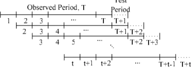
suggestion of Basle Capital Accord (BCA) in 1996, we use the “Backtesting” method to evaluate the reliability of our model. Let T denote the observed period in Figure 3. Each window consists of T observed values and 1 test value in the Sliding Window Methodology. The sliding window shifts one time slot gradually until the end of our experiment. Substituting these T observed values into Equation (3)-(5), the VaRi is calculated. Comparing VaRi and

actual return data in test value, it means success if VaRi is larger, otherwise, it means failure. After

shifting t times of sliding window, the Success Rate is defined as follows. t Success of Number Rate Success = (6)

In our experiment, T contains 764 samples in each window, the sliding window shifts 100 times (t=100) and the overall experiment period is from 1987 to 2004.

Figure 3. Sliding window simulation process

The parameters used in GA are set as follows: the population size is 100, the chromosome length is 170

(5*34), the number of generations is 500, the crossover rate is 0.6 and the mutation rate is 0.001. Besides, the selection method is roulette wheel and the crossover method is one-point crossover.

Three experiments A, B, and C. with 90%, 95%, and 99% significance confidence level, respectively, are listed in Table 1, where higher confidence level select less assets and vice versa. For example: 10, 4 and 2 assets are selected if considering 99%, 95% and 90% confidence level, respectively. PVaR in Table 1 are 6.58, 7.09, and 10.46. It shows that higher confidence level produces larger PVaR. Furthermore, higher confidence level avoids undervaluing risk in whole portfolio, such as experiment B and C, where their success rates are larger than confidence levels.

Table 1. The optimal portfolio’s VaR for empirical distribution

Experiment Num. of stock _{success rate}Portfolio Confidence level _{(1-P) estimation} Risk PVaR

A 10 85.23% 90% Undervalued 6.58 B 4 98.75% 95% Overvalued 7.09 C 2 100.00% 99% Overvalued 10.46 The experiment B is listed in detail in Table 2.

We find the GPD approxiamtion to be preferable, because it can deal with asymmetries in the fat-tailed with ξ>0 and β>0. Table 2. The detail individual VaR in portfolio with 95% confidence level

Selected Assest Success rate Threshold ui VaRi pi βi ξi

X1 98% -6.34 10.04 0.14 0.23 0.010 X2 97% -5.43 4.13 0.15 0.22 0.001 X3 100% -5.22 5.26 0.09 0.29 0.003 X4 100% -6.88 8.92 0.06 0.22 0.025 average 98.75% -5.97 7.09 0.12 0.24 0.010 4. Conclusion

Forecasting volatility of portfolio is important in investment decision. Conventionally, to forecast PVaR and select efficient set of portfolio should be seriously limited if using statistical linear model under specific assumptions. Traditional risk management model might fail to forecast VaR precisely because of estimating tail distribution incorrectly. Most real financial time series data is fat-tailed distribution. EVT model is proven to be a powerful method in risk forecasting by focusing directly on the distribution of extreme returns instead

of whole the distribution of all returns. However, forecasting the PVaR is very difficult because EVT provides less maturity on analyzing multivariate model. In this article, a GA based PVaR forecasting mechanism under EVT model is introduced, where GA mechanism extracts an efficient portfolio set, and estimates more suitable peak threshold values for all assets to forecast more precise PVaR, simultaneously. From 34 companies listed and traded in the TSE, we try to demonstrate the stability and robustness of our mechanism. The preliminary results show that higher confidence level produces larger PVaR. Furthermore,

it also shows that higher confidence level effectively avoids undervaluing risk in whole portfolio, because undervaluing risk will lead to possible financial distress or bankruptcy.

REFERENCES

[1] H. Markowitz, “Portfolio selection”, Journal of Finance, Vol. 7, pp.77-91, 1952.

[2] H. N. E. Bystrom, “Managing extreme risks in tranquil and volatile markets using conditional extreme value theory,” International Review of Financial Analysis, Vol. 13, pp. 133-152, 2004. [3] J. Holland: Adaptation in Natural and Artificial

Systems: An Introductory Analysis with Applications to Biology, Control and Artificial Intelligence. (University of Michigan Press, 1975).

[4] J. Shoaf and J. A. Foster, “The efficient set GA for stock portfolios,” In Proceedings of IEEE International Conference on Computational Intelligence, pp. 354 – 359, 1998.

[5] K. F. C. Yiu, “Optimal portfolios under a value-at-risk constraint,” Journal of Economic Dynamics & Control, Vol. 28, pp. 1317-1334, 2004.

[6] P. M. Arenas, T. A. Bilbao, and U. M. V. Rodríguez, “A fuzzy goal programming approach to portfolio selection,” European Journal of Operational Research Vol. 133, pp. 287-297, 2001.

[7] R. Campbell, R. Huisman and K. Koedijk, “Optimal portfolio selection in a value at risk framework,” Journal of Banking & Finance, Vol. 25, pp. 1789-1804, 2001.

[8] R. Gencay, F. Selcuk and A. Ulugulyagci, “High volatility, thick tails and extreme value theory in value-at-risk estimation,” Insurance: Mathematics and Economics, Vol. 33, pp. 337-356, 2003.

[9] S. Gnaganelli and R. F. Engle, “Value at risk models in finance,” Working paper no. 75, European Central Bank, 2001.

[10] S. H. Poon and C. Granger, “Forecasting volatility in financial markets: a review,” Vol. 41, pp.478-539, 2003.

[11] Y. Crama and M. Schyns, “Simulated annealing for complex portfolio selection problems,” European Journal of Operational Research Vol.150, pp.546-571, 2003.

[12] Y. Xia, B. Liu, S. Wang, and K. K. Lai, “A Model for Portfolio Selection with Order of Expected Returns," Computers & Operations Research, 27, pp.409-422, 2000.

[13] Y. Xia, S. Wang and X. Deng, “A Compromise solution to mutual funds portfolio selection with transaction costs,” European Journal of Operational Research, Vol. 34, pp. 564-581, 2001.