經由混合方法進行管線化快速傅利葉轉換處理器的字元長度最佳化之研究

全文

(1)國立交通大學電機資訊學院電子與光電學程. 碩. 士. 論. 文. 利用混合方法進行管線化快速傅利葉轉換處理器的字元長度最佳化之研究 Hybrid Wordlength Optimization Methods of Pipelined FFT Processors. 研究生 : 指導教授 :. 郭志彬周景揚教授. 中華民國九十三年. 八月.

(2) 利用混合方法進行管線化快速傅利葉轉換處理器的字元長度最佳化之研究 Hybrid Wordlength Optimization Methods of Pipelined FFT Processors 研究生: 郭志彬指導教授: 周景揚. Student : Chih-Bin Kuo Advisor : Jing-Yang Jou. 國立交通大學. 電機資訊學院電子與光電學程碩. 士. 論. 文. A Thesis Submitted to Degree Program of Electrical Engineering Computer Science. College of Electrical Engineering and Computer Science National Chiao Tung University in Partial Fulfillment of the Requirements for the Degree of Master of Science in Electronics and Electro-Optical Engineering August 2004 Hsinchu, Taiwan, Republic of China. 中華民國九十三年. 八月.

(3) 利用混合方法進行快速傅利葉轉換處理器的字元長度最佳化之研究研究生：郭志彬. 電機資訊學院. 指導教授：周景揚教授國立交通大學電子與光電學程 (研究所) 碩士班. 摘要快速傅利葉轉換處理器是許多通訊系統中的關鍵元件，利用快速傅利葉轉換處理器的設計自動化，可減輕系統設計的時程壓力。在設計管線化快速傅利葉轉換處理器時，處理級(Process Element)的字元長度是重要的參數。在本篇論文中，我們提出關於管線化快速傅利葉轉換處理器每一級的字元長度對訊號對量化雜訊比(SQNR)的統計學模型。更進一步地，提出透過混合使用統計與模擬誤差分析的管線化快速傅利葉轉換處理器字元長度的最佳化流程。在系統設計者所提供的快速傅利葉處理器點數、訊號對量化雜訊比和處理器速度限制條件下，本方法可於數秒內自動地產生一組最佳化的字元長度參數。實驗的結果顯示，此快速的最佳化流程可縮小 8192 點管線化快速傅利葉轉換處理器面積達 24%。. i.

(4) Hybrid Wordlength Optimization Methods of Pipelined FFT Processors Student: Chih-Bin Kuo. Advisor: Dr. Jing-Yang Jou. Degree Program of Electrical Engineering Computer Science National Chiao Tung University. Abstract The Fast Fourier Transform (FFT) processor is a key component in many communication systems. To reduce design time of FFT processors through design automation is to reduce the time pressure of system designers. When implementing a pipelined FFT processor the wordlength is of great importance. This thesis describes a statistical error model of pipelined FFT processors that calculates the signal to quantization noise ratio (SQNR) with wordlength of each process element (PE) stage. Furthermore, to speed up the design of specified FFT processor, a hybrid optimization method with statistical and simulation-based error analysis is presented. Under constraints of the number of FFT points, SQNR, and required processors speed, the optimized wordlength set for each PE stage can be generated within several seconds. The experimental results designate that this speedy flow can reduce 24% area of 8192-point pipelined FFT processors.. ii.

(5) Acknowledgement I would like to express my heartfelt gratitude to my advisor, Professor Dr. Jing-Yang Jou, for his guidance and encouragement throughout the three-year graduate course. I also deeply appreciate Assistant Professor Dr. Juinn-Dar Huang for his constructive suggestion on this thesis. Special thanks to all the EDA members for the wonderful time we share together. Finally, I display my warmest appreciation to my parents and my dear Juno and A-Kang for their love and support.. iii.

(6) Contents 摘. 要. i. ABSTRACT. ii. ACKNOWLEDGEMENT. iii. CONTENTS. iv. LIST OF TABLES. vii. LIST OF FIGURES. viii. Chapter 1. Introduction……………………………………………………………….. 1. Chapter 2. Review of FFT…………………………………………………….....…...... 4. FFT Algorithms……...………………………………………………............. 4. 2.1.1. Basic Concepts of FFT Algorithms……………………….......…...... 5. 2.1.2. Fixed-Radix FFT Algorithms……………………………………...... 6. 2.1. 2.1.2.1. Radix-2 Algorithm………………………………………..…. 6. 2.1.2.2. Radix-4 Algorithm………………………………………...…. 7. 2.1.2.3. Radix-22 Algorithm……………………………………….…. 8. Split-Radix FFT Algorithms…………………………………....….... 9. FFT Architectures……………………………………………………............. 9. 2.1.3 2.2 Chapter 3. Error Analysis……….……………………………………………………. 13. 3.1. Error Analysis of Quantization………………………….…………............... 13. 3.2. Statistical Error Models of FFT…..………………...……………………….. 15 3.2.1. Definitions and Constraints………….……………………………... 16. 3.2.2. Expected Noise Sources…….……….……………………………... 17. 3.2.3. Output SQNR……………….……….……………………………... 18. iv.

(7) 3.3. Simulation-Based Error Analysis of FFT....……….…………..……………. 22. 3.4. Verifications……………………….....…………………………………….... 22. Chapter 4. 3.4.1. Random Verification…….………….…………………………..…... 23. 3.4.1. Partial Exhaustive Verification…….…………………………...…... 25. Wordlength Optimization……….……………………………………….. 26. 4.1. FFT Processor Design Flow…………………………………………............ 26. 4.2. Wordlength Generation………………………………………………….….. 28 4.2.1. Library and Table…..…….………….………………………….…... 28. 4.2.2. Upper Bound Wordlength Evaluation.……………………………... 29. 4.2.3. Lower Bound Wordlength Evaluation.……………………………... 30. 4.2.4. Optimized Wordlength Candidate (OWC) Searching…………….... 32. 4.2.5 4.3. Chapter 5. 4.2.4.1. Optimization Format…..………………………………….… 32. 4.2.4.2. OWC Searching Flow….…………………………………… 33. Optimized Wordlength (OW) Selection.………………………….... 34. Examples of Wordlength Optimization……………………….…………….. 36 4.3.1. Hybrid Method.…………………………………………..….……... 36. 4.3.2. Pure Statistical Method.…………………………..…………….…... 37. Experimatal Results…………………………………………………...…. 38. 5.1. Introduction…………………………………..………………………….….. 38. 5.2. Results…………………………………………………………………...….. 38 5.2.1. Optimization of Different Constraint……………………..………... 39 5.2.1.1. FFT Point…..…………………………..………………….… 39. 5.2.1.2. Input Wordlength and Output Wordlength…………..……… 41. 5.2.1.3 SQNR…………………………………………………..…… 43. v.

(8) 5.2.1.4 SQNR Error………………………………………………… 44 5.2.2. 5.2.3. Chapter 6. Special Cases of Optimization ……………………..………….…... 45 5.2.2.1. Absolute Constraint Over …………………...……………… 45. 5.2.2.2. Partial Constraint Over ……………………………...……… 46. Methods Comparison ……………………..…………………...…... 47 5.2.3.1. Previous Work vs. Our Work …………………………..…… 47. 5.2.3.2. Our Hybrid Method vs. Pure Statistical Method…….……… 48. Conclusions and Future Work……………………………………..……. 49. References……….……………………………………………………………………… 50 Vita……..……….…………………..…………………………………………………… 52. vi.

(9) List of Tables Table 2.1. Summary of N Point Pipelined FFT Architecture……………………. 11. Table 3.1. Examples of Random Verification (N=1024)……….……………….. 22. Table 5.1. Specification of Common FFT for OFDM…………………………... 39. Table 5.2. Area Optimization of Different FFT Point (IO Wordlength =18)……. 40. Table 5.3. Area Optimization of Different FFT Point (IO Wordlength =14)……. 42. Table 5.4. Area Optimization of Different FFT Point (SQNR Error = 1.1dB)….. 45. vii.

(10) List of Figures Figure 1.1. Architecture View of OFDM................................................................ 1. Figure 2.1. Symmetric Property of Twiddle Factor................................................. 5. Figure 2.2. Butterfly Graph of Radix-2 DIF FFT.................................................... 6. Figure 2.3. Signal Flow Graph of 16 Point Radix-2 DIF FFT................................ 7. Figure 2.4. Butterfly Graph of Radix-4 DIF FFT.................................................... 8. Figure 2.5. Butterfly Graph of Radix- 2 2 DIF FFT.................................................. 8. Figure 2.6. R2MDC Architecture (N=16)............................................................... 10. Figure 2.7. R2SDF Architecture (N=64)................................................................. 10. Figure 2.8. R4MDC Architecture (N=256)............................................................. 10. Figure 2.9. R4SDF Architecture (N=64)................................................................. 11. Figure 2.10. R2 2 SDF Architecture (N=64).............................................................. 11. Figure 2.11. Units of R2SDF and R22SDF........………………................................ 12. Figure 3.1. Information of 2+1 Bits Quantizer…………........................................ 15. Figure 3.2. Error Model of PE Stage……………………...................................... 17. Figure 3.3. Propagating Flow of Quantization and Scaling Errors......................... 19. Figure 3.4. Propagating Flow of Multiplication Errors……………....................... 19. Figure 3.5. Propagating Flow of Noiseless Multiplication..................................... 21. Figure 3.6. Simulation Environment of SQNR……………................................... 22. Figure 3.7. Results of Random Verification of Radix-2 and Radix-22................... 24. Figure 3.8. Results of Partial Exhaustive Verification of Radix-2 and Radix-22.... 25. Figure 3.9. Two Examples of Wordlength Optimization......................................... 37. Figure 4.1. Design Flow of FFT Processors .........…………….............................. 27. Figure 4.2. Over All Flow of Wordlength Optimization......................................... 28. viii.

(11) Figure 4.3. Flow of Upper Bound Wordlength Evaluation..................................... 30. Figure 4.4. Flow of Lower Bound Wordlength Evaluation..................................... 31. Figure 4.5. Example of Lower Bound Wordlength Evaluation............................... 32. Figure 4.6. Area Increment of Add Wordlength 1 Bit of Each Stage...................... 33. Figure 4.7. Flow of Optimized Wordlength Candidate Searching.......................... 34. Figure 4.8. Flow of Optimized Wordlength Selection............................................ 35. Figure 4.9. Example of Hybrid Wordlength Optimization Method........................ 36. Figure 4.10. Example of Pure Statistical Wordlength Optimization Method............ 37. Figure 5.1. Area Reduction Rate of IO Wordlength 18 and 14 Bits....................... 43. Figure 5.2. Area Reduction Rate vs. SQNR Constraint.......................................... 44. Figure 5.3. Output Message of Generator when There is No Solution................... 46. Figure 5.4. Output Message of Generator when There is No Solution................... 46. Figure 5.5. Comparison Result between Simulation-Based and Hybrid Method... 47. Figure 5.6. Comparison Result between Hybrid and Pure Statistical Method........ 48. ix.

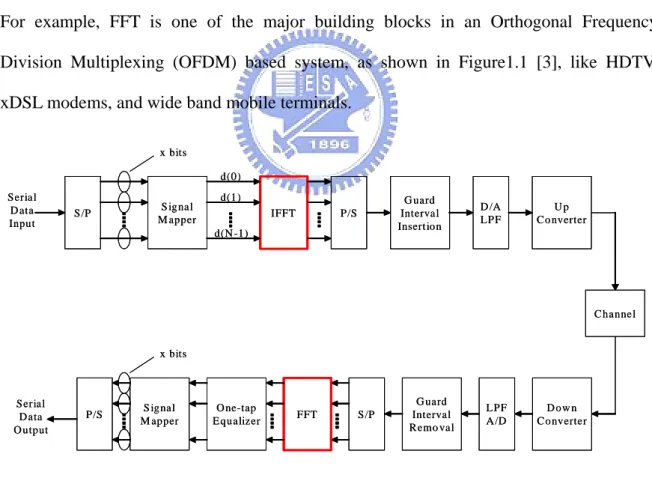
(12) Chapter 1 Introduction The FFT is one of the most widely used digital signal processing algorithms. Recently, attention has been returned to real-time FFT processors in many communication systems. For example, FFT is one of the major building blocks in an Orthogonal Frequency Division Multiplexing (OFDM) based system, as shown in Figure1.1 [3], like HDTV, xDSL modems, and wide band mobile terminals. x bits d(0). Serial D ata Input. S/P. S ignal M apper. d(1). IFFT. G uard Interval Insertion. P/S. d(N -1). D /A LPF. Up Co nverter. Channel. x bits. Serial D ata O utput. P/S. S ignal M apper. O ne-tap Equalizer. S/P. FFT. G uard Interval Remo val. LPF A/D. D ow n Converter. Figure 1.1 Architecture View of OFDM. There are many possible architecture choices for FFT processors. Among them, the pipelined FFT architectures that are particularly suitable for real-time applications since it. 1.

(13) can easily be merged with the sequential nature of sampling. It is suitable for VLSI technology progresses because it is regular and its control circuit is easy to implement. In the pipelined FFT architectures, the most research effort has been relative to the regular module implementations, which uses fixed wordlength for both data and coefficients for each stage. The possibility to use different wordlength is often ignored to achieve modulized solutions. However the fast growing use of Intellectual Property (IP) makes the non-module implementation viable, which allows us to exploit the pipeline architectures further. The wordlength may affect the precision, quantization error, and complexity of hardware. The increased wordlength will increase the precision and decrease the quantization error at the cost of area and power. On the other hand, to maintain a lower hardware cost, a shorter wordlength may be chosen at the sacrifice of the precision. In general, a FFT can’t be implemented exactly. Each multiplier and adder in pipelined FFT architectures may introduce an error caused by the rounding or truncation of the arithmetic results. Errors will accumulate successively over the FFT stages. The error introduced at the early stages may influence the performance in the later stages. Therefore, it is required to find an optimized solution of wordlength in pipelined FFT processors. The statistical method and simulation-based method are popular for FFT error analysis between signal-to-quantization-noise ratio (SQNR) and wordlength. The SQNR can be calculated quickly by statistical model. With the advent of more powerful computers recently, SQNR of different algorithms and different architectures can be accurately simulated. Stage level statistical error analysis method of pipelined FFT processor will be presented in this thesis. Furthermore, a hybrid wordlength optimization method of pipelined FFT processor will be introduced. The wordlength parameters of each stage are. 2.

(14) generated automatically by using the constraints of point of FFT, SQNR, and throughput of processors. The rest of this thesis is organized as follows. In Chapter 2, a brief review of FFT algorithms and architectures is given. Error analysis methods are introduced in Chapter 3. In Chapter 4, the wordlength optimization of our approach is presented step-by-step. The experimental results are then presented in Chapter 5. Finally, the conclusions and the future works are given in Chapter 5.. 3.

(15) Chapter 2 Review of FFT Substantial literatures are available on algorithm and architecture of FFT. In this chapter, we will briefly review some popular types of algorithms of FFT. And we will introduce architectures of FFT.. 2.1. FFT Algorithms The Discrete Fourier Transform (DFT) plays a significant role in the region of digital. signal processing (DSP) and communications. However, the computational complexity of direct evaluation of an N-point DFT is O( N 2 ) , which costs a long computation time and large power. Thus, there is a great requirement to develop a fast DFT algorithm. Many FFT algorithms have been derived to reduce computation complexity, such as Cooley-Turkey algorithm [1] [2], Rader algorithm [2], and Winograd algorithm [2]. Among them, the Cooley-Turkey algorithm is very popular because it can reduce the computational complexity from O( N 2 ) to O( N log 2 N ) , and the regularity of the algorithm makes it suitable for VLSI implementation. It will be discussed in this section.. 4.

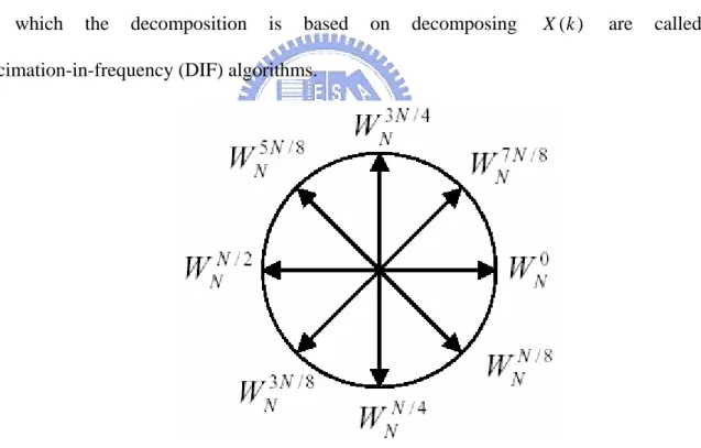
(16) 2.1.1 Basic Concepts of FFT Algorithms FFT algorithms are approaches to compute DFT. The formulation of N length DFT is define as equation (2.1). N −1. X ( k ) = ∑ x ( n )WNnk , k = 0,1,......., N − 1. (2.1). n =0. where the coefficient WNnk is defined as equation (2.2) and is called twiddle factor, and the W. nk N. =e. − j 2πnk N. = cos(. 2πnk 2πnk ) − j sin( ) N N. (2.2). symmetric property is showed in Figure 2.1. The X (k ) is in frequency domain, and x(n) is in time domain. Algorithms in which the decomposition is based on decomposing x (n ) term are called decimation-in-time (DIT) algorithms. On the other hand, algorithms. in. which. the. decomposition. is. based. on. decomposing. X (k ). decimation-in-frequency (DIF) algorithms.. Figure 2.1 Symmetric Property of Twiddle Factor. 5. are. called.

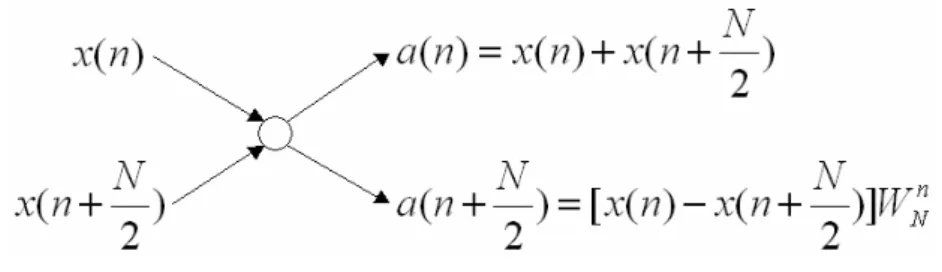
(17) 2.1.2. Fixed-Radix FFT Algorithms. Fixed-Radix algorithms include the radix-2, radix-4/radix-22, radix-8/radix-23, etc. Among them, the radix-2 algorithm is the simplest one. The radix-4 algorithm has the smallest multiplicative complexity. And the radix-22 has benefits of radix-2 and radix-4. They will be reviewed in this section.. 2.1.2.1 Radix-2 Algorithm The radix-2 algorithm is using the divide-and-conquer approach with which algorithm is dividing the problem of N point FFT, where N is power-of-2, by factor of 2. With the symmetric property of equation (2.2), WNnk = −WNnk + N / 2 , the equation (2.3) will be founded. A × W Nnk + B × W Nnk + N / 2 = ( A + B × W NN / 2 ) × W Nnk = ( A − B ) × W Nnk. (2.3). By using the property of equation (2.3), the summation of equation (2.1) can be divided into two summations in equation (2.4), and it is the equation of radix-2 DIF. X (2r ) =. N / 2 −1. ∑ [ x(n) + x(n + N / 2)]W. nr N /2. n =0. X (2r + 1) =. N / 2 −1. ∑ [ x(n) − x(n + N / 2)]W n=0. n N. W Nnr/ 2 ,. r = 0,1,..., ( N / 2) − 1. (2.4). The addition and the subtraction operation of x(n) and x ( n + N / 2) in equation (2.4) are called the butterfly (BF) operation as shown in Figure 2.2. After log2N - times recursive decomposing, the complete radix-2 DIF algorithm can be obtained. Figure 2.3 shows the Signal Flow Graph (SFG) of N=16 radix-2 DIF algorithm FFT.. Figure 2.2 Butterfly Graph of the Radix-2 DIF FFT 6.

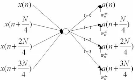
(18) Figure 2.3 SFG of 16 Point Radix-2 DIF FFT. 2.1.2.2 Radix-4 Algorithm There is another symmetry property of equation (2.2) shown in equation (2.5). W Nnk + N / 4 = −W Nnk +3 N / 4 = − jW Nnk. (2.5). Because of the –j term, we only need to exchange 2’s complement of real part data and image part data instead of applying multiplication operation. The arithmetic cost can be reduced. The equation of radix-4 DIF [4] is shown in equation (2.6). X (4r + l ) =. N / 4 −1. ∑ [ x(n) + x(n + n =0. 3N N N ) × W4l + x ( n + )W42 l + x ( n + ) × W43l ]WNnlWNnr/ 4 , 4 2 4 r = 0,...,. N − 1 , l = 0,1,2,3 4. The mapping butterfly graph of equation (2.6) is shown in Figure 2.4.. 7. (2.6).

(19) Figure 2.4 Butterfly Graph of Radix-4 DIF FFT. 2.1.2.3 Radix-22 Algorithm If we further divide the equation (2.6), we can get the equation (2.7) of radix-22 [4]. It implements the radix-4 BF by two radix-2 BFs. The mapping butterfly graph of equation (2.7) is shown in Figure 2.5. X (4r + 2l 2 + l1 ) = X (4r + 2l2 + l1 ) =. N / 4 −1. ∑ [ x ( n) + x ( n + n =0. N / 4 −1. ∑ n =0. [ x ( n) + x ( n +. N N 3N ) × W42l2 +l1 + x(n + )W44l2 + 2l1 + x(n + ) × W46l2 +3l1 ]W Nn ( 2l2 +l1 )W Nnr/ 4 , 4 2 4 3N N N ) × W42l2 + l1 + x(n + )W44l 2 + 2l1 + x(n + ) × W46l2 + 3l1 ]WNn ( 2l 2 + l1 )WNnr/ 4 4 2 4. r = 0,...,. N − 1 , l1 = 0,1 4. l2 = 0,1. 2. Figure 2.5 Butterfly Graph of Radix- 2 DIF FFT. 8. (2.7).

(20) 2.1.3 Split-Radix FFT Algorithms The computation cost of the Fixed-Radix algorithm FFT can be further reduced by combining radix-2 and radix-4 or radix-2 and radix-8, called Split-Radix algorithm. It has fewer multiplications and additions. So, they have advantage on computational complexity. But, they are not regular as radix-2r algorithms and seldom used in ASIC design. The most popular split-radix algorithms are proposed by Duhamel et al. [5].. 2.2. FFT Architectures The FFT is one of the most widely used digital signal processing algorithms. Recently,. attention has been returned to real-time processors in many communication systems. There are many architecture choices for these processors. Among them, the pipelined architectures are particularly suitable for real-time applications since they are easily merged with the sequential nature of sampling. And they are popular for large FFT VLSI realization too, due to their high regularity. In this section, we will introduce the pipeline-based architecture. The architecture that we want to discuss is used to implement DIF FFT algorithms. Similar structures can be designed for DIT FFT algorithms, too. Several architectures for pipelined FFT processors have bean proposed. There are Radix-2 Multi-path Delay Commutator (R2MDC) [6], Radix-2 Single-path Delay Feedback (R2SDF) [7], Radix-22 Single-path Delay Feedback (R22SDF) [8][9], Radix-4 Single-path Delay Feedback (R4SDF) [6], Radix-4 Multi-path Delay Commutator (R4MDC) [6], etc. They will be introduced in this section.. 9.

(21) z R2MDC It is the most straightforward way to reorganize the data for FFT algorithms. At each stage half the data stream is delayed via the memory and processed with the second half data stream. An 16-point R2MDC is shown in Figure 2.6. 4. 8. C2. C2. PE. x. 2 PE. PE. C2. x. 4. 1. 2. PE. C2. 1. -j. Figure 2.6 R2MDC Architecture (N=16). z R2SDF Since memory in R2MDC is idle at 50% of time, it can be reused as shown in Figure 2.7 This scheme utilizes the different arrival time of input data and processed data. The utilization of the memory is 100%. 32 PE. PE. x. x. 2. 4. 8. 16. PE. x. PE. 1. PE. x. PE. -j. Figure 2.7 R2SDF Architecture (N=64). z R4MDC It is similar with R2MDC, but it utilizes only 25% of time for memory. A 256-point R4MDC is shown in Figure 2.8. 192 128 C4 64. PE. x x x. 16 32 48. C4. 48 32 16. PE. x x x. 4 8 12. C4. 12 8 4. PE. Figure 2.8 R4MDC Architecture (N=256). 10. x x x. 1 2 3. C4. 3 2 1. PE.

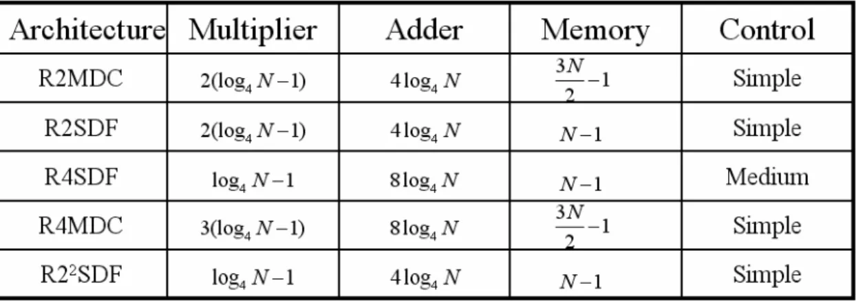
(22) z R4SDF It is a radix-4 version of R2SDF. It is as efficient as R2SDF in terms of memory utilization and the utilization of multipliers increases from 50% to 75% at a cost of only 25% utilization of the BF element. A 64-point R4SDF is shown in Figure 2.9. 16 16 16. 4 4 4. 1 1 1. PE. PE. PE. x. x. Figure 2.9 R4SDF Architecture (N=64). z R22SDF It breaks one radix-4 BF operation into two radix-2 BF operation with trivial multiplications of ± 1 and ± j . With a feedback mechanism, the memory is fully utilized as R2SDF and R4SDF. A 64-point R22SDF is shown in Figure 2.10. 16. 32 PE. -j. PE. 8. x. 4. PE. -j. PE. 2. x. PE. 1. -j. 2. Figure 2.10 R2 SDF Architecture (N=64). Table 2.1 Summary of N Point Pipelined FFT Architectures. 11. PE.

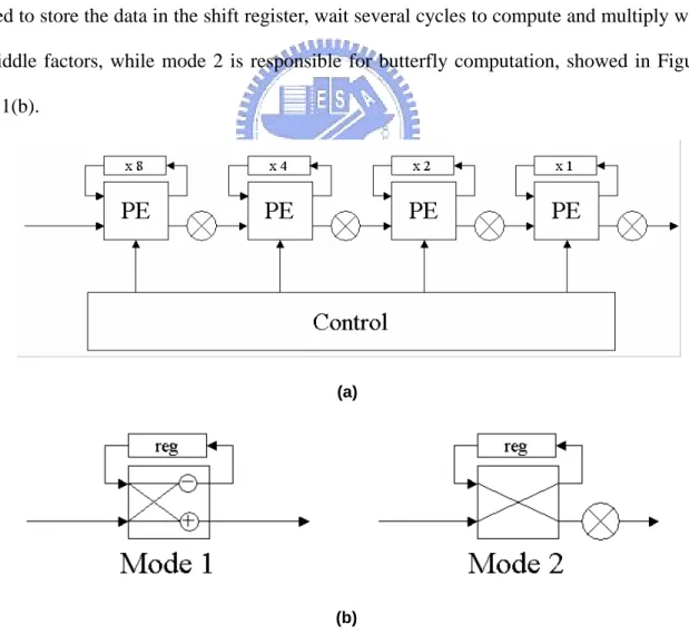
(23) Summary of these architectures are shown in Table 2.1 [5]. The delay feedback approached are always more efficient than corresponding delay commutator approaches in terms of memory requirements. The Radix-4 algorithm based single-path architectures have fewer multipliers than those of radix-2 algorithm. However, radix-2 algorithm based architectures have properties of simple and regular. And radix-22 algorithm is characterized with the trait that it has same multiplicative complexity as radix-4 algorithms but still retains the radix-2 butterfly structure. In this thesis we will focus on R2SDF and R22SDF architectures. The detail architecture with control unit of R2SDF and R22SDF is shown in Figure 2.11(a). The butterfly process element (PE) has two kinds of operation modes. Mode 1 is used to store the data in the shift register, wait several cycles to compute and multiply with twiddle factors, while mode 2 is responsible for butterfly computation, showed in Figure 2.11(b).. (a). (b) Figure 2.11 Units of R2SDF and R22SDF (N=16). 12.

(24) Chapter 3 Error Analysis Fixed-point arithmetic is popular for FFT hardware implementation for its simplicity. Because of the finite wordlength in the computation, we have to truncate or round the answers when overflow occurs after addition or multiplication; thus, errors are produced. The statistical error analysis and simulation-based error analysis are the two most popular methods for FFT error analysis. Many papers about statistical and simulation-based error analysis of fixed-point FFT have been published [10-14]. The previous statistical error analysis is not sufficient for our purpose of choosing the required wordlength stage by stage. We derive a simplified statistical error model to meet the requirement. In this chapter, we will briefly review the quantization error analysis first. Second, we will introduce the statistical error models in which wordlength can be freely chosen stage by stage. Third, the simulation environment will be briefly reviewed. Then accuracy of our error models will be evaluated by comparing it with that of the simulation-based error analysis.. 3.1 Error Analysis of Quantization The basic formula for the quantization error analysis is shown below. Let X be a 13.

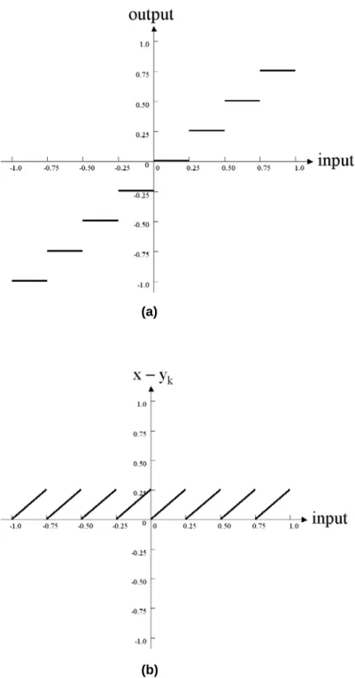
(25) finite-length sequence {x(n)} ; n = 0,1,2,..., N − 1 . The expected value of X is shown in equation (3.1). It is zero-mean random sequence at the quantizer input. The variance of X is denoted by σ x2 and is shown in equation (3.2).. µ x = E[ X ] =. 1 N. σ x2 = E[ X 2 ] =. N −1. ∑ x(n) =0. (3.1). n=0. N −1. 1 N. ∑ [ x(n) − µ n=0. x. ]2. (3.2). where the E[⋅] in equation (3.1) and (3.2) is the expected value operator. A quantizer Q (⋅) maps X into the discrete-valued Y. Thus, the quantization error Q = X − Y . Denote the boundaries by {bk }kM=0 and the reconstruction levels by { y k }kM=1 ,. then the output of this quantizer is shown in equation (3.3) and the quantization error variance, denoted by σ q2 , is then given by equation (3.4). Y = Q( x) = yk. σ q2 = E[Q 2 ] =. bk −1 < x ≤ bk. iff 1 N. M. (3.3). bk. ∑ ∫[x − y k =1 bk −1. k. ] 2 dx. (3.4). Finally, the equation of SQNR is shown in equation (3.5). SQNR =. σ x2 σ q2. (3.5). For example, if the input is uniformly distributed in the interval (-1, 1) and the output is 2 + 1 bits sign-fractional discrete-valued data. The input-output mapping is shown in Figure 3.1(a). It is shown that, if the input data are in the interval [0,0.25) then the output data of them are all have the same value as 0. If the input data are in the interval [0.25,0.5) then the output data of them are 0.25, and so on. The related quantization error mapping is shown in Figure 3.1(b).. 14.

(26) (a). (b) Figure 3.1 Information of 2+1 Bits Quantizer. 3.2 Statistical Error Models of FFT The previous FFT error analysis and model of DIF radix-2 algorithm have been presented by Sundaramurthy et al. [12] . They assume that all the wordlength of all PE stages is the same. This is insufficient for applications that allow the different wordlength. 15.

(27) between PE stages. Due to the finite wordlength in the computation, we have to truncate or round the answers after calculation. And the FFT computation is an iterative process and the value increases in magnitude. The problem of overflowing should be concerned. In order to prevent overflow and to ensure output accuracy, data need to be scaled. There are two scaling methods to prevent FFT from overflow. One is overall scaling and the other is stage-by-stage scaling [2]. The input constraint of FFT with overall scaling is x(n) <. 1 , and there is no need to divide the input of each butterfly by two. The input N. constraint of FFT with stage-by-stage scaling is x(n ) < 1 , and the input data should be divided by 2 for each butterfly. Due to the noise consideration [14] the stage-by-stage scaling will be used in this thesis. In this section we aim on delivering statistical FFT error models for DIF radix-2 and radix-4 algorithms with stage-by-stage scaling scheme. These models are useable for case having the different wordlength stage by stage.. 3.2.1 Definitions and Constraints In these analyses, we assume fixed-point arithmetic with (bk + 1) bit wordlength and signed fraction, where k is the stage number of PE stage. The input of N-point FFT, denoted by x(m) where m = 0,1,2,..., N − 1 , is a sequence of finite valued complex numbers. Numbers are consisted by 2N real random variable and they are uncorrelated. And they are distributed uniformly in (. −1 2. ,. 1 2. ) . Note the range of (. −1 2. ,. 1 2. ) is. consistent with the condition that x(m) < 1 for all m. The effect of the inaccuracy in the twiddle factor, W p , is not treated here. The truncation operations are all modeled as mutually uncorrelated.. 16.

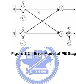
(28) 3.2.2 Expected Noise Sources Figure 3.2 shows the error model of PE stage with stage-by-stage scaling by 2. There are several noise sources having been considered. They are the quantization error of wordlength difference between PE stages, denote by σ q2k , the quantization error of scaling, denoted by σ s2k , the quantization error of complex multiplication of twiddle factor, denoted by σ m2 k , and the insufficient output wordlength error, denoted by σ Q2o .. Figure 3.2 Error Model of PE Stage. z. σ q2 and σ s2 k. k. The σ q2k is produced when the wordlength of stage k-1, denoted by bk -1 , is greater then that of stage k, denoted by bk . σ q2k is the variance of truncated bits from bk -1 to bk . The scaling error is produced when bk < bk -1 + 1 . A complex scaling consists of two real scaling, i.e., the real and imaginary parts of the number are scaled separately. Scaling by a factor. 1 involves a 1-bit right shift and truncation of the last bit. σ s2k is the variance of 2. this bit. The sum of errors σ q2k and σ s2k can be replaced as the error of directly scaling the data of stage k-1 then truncate to bk . This new error is denoted by σ s2k to replace the combination error of old σ s2k and σ q2k . It is shown in equation (3.6). 17.

(29) σ. z. 0 ⎧ ⎪ = ⎨ 1 -2(b +1) M-1 2 k -1 ⋅ ∑v ) ⎪⎩2( M ⋅ 2 v =0. 2 sk. ; b k -1 + 1 ≤ b k , M = 2 (bk -1 +1)-b k. ; b k -1 + 1 > b k. (3.6). σ m2. k. It is assumed that a complex multiplication is implemented by four real multiplications and each real multiplication is truncated separately. The complex multiplication error variance, denoted by σ m2 k , is equal to the variance of truncated bits of the result of multiplication. It is shown in equation (3.7).. σ. z. 2 mk. ⎧ 1 -2⋅(bk -1 +1+ bk ) M-1 2 ⋅ ∑v ) ⎪⎪ 4( M ⋅ 2 v =0 =⎨ M -1 1 ⎪ 4( ⋅ 2 -2⋅2b k ⋅ ∑ v 2 ) ⎪⎩ M v =0. , M = 2 (bk -1 +1+ bk )-b k. ; b k -1 + 1 ≤ b k. (3.7) ,M =2. 2b k -b k. ; b k -1 + 1 > b k. σ q2. o. If the output wordlength is small then the output wordlength of the last PE stage the quantization error will be produced. The variance σ Q2o is shown in equation (3.8), where the bL is the wordlength of the last PE stage and the bo is the FFT output wordlength.. σ. 2 qo. 0 ⎧ ⎪ = ⎨ 1 -2b M-1 2 L v ) ⎪⎩2( M ⋅ 2 ⋅ v∑ =0. ; bL ≤ bo , M = 2 b L -bo. ; bL > bo. (3.8). 3.2.3 Output Signal to Quantization Noise Ratio (SQNR) Since all the noise sources are assumed to be uncorrelated, the variance of the noise at output node of the SFG of Figure 2.5 is the sum of contributions from all the individual noise sources that propagate to that output node. Some of noise variance of output nodes 18.

(30) that is contributed by σ s2k is denoted by σ S2 , and the contribution of σ m2 k is denoted by. σ M2 . From Figure 3.3, the propagation of σ s2k in 8-point DIF Radix-2 it can be found. The number of error source σ s2k propagating to any output node from the first, second, and third stage are 8, 4, and 2, respectively. And the equation of σ S2 is shown below, equation 1 (3.9), where the total stage number n is equal to log2N, and the factor of ( ) n− k is the 4. effect of scaling on the error propagating at stage k. The σ S2 of DIF Radix-22 algorithm is the same as DIF Radix-2.. Figure 3.3 Propagating Flow of Quantization and Scaling Errors. 1 4. σ S2 ≈ N ( ) n −1 ⋅ σ s2 + 1. N 1 n−2 2 N 1 ( ) ⋅ σ s2 + L + n −1 ( ) n − n ⋅ σ s2n 2 4 2 4. (3.9). It can be assumed that all the complex multiplications are noisy for convenience of derivation. Figure 3.4 show that the propagation of σ m2 k in 8-point DIF Radix-2 algorithm 19.

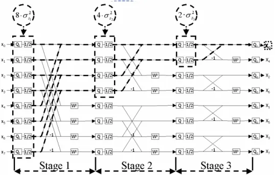
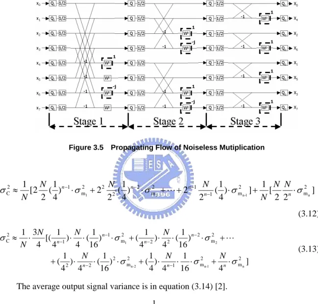
(31) SFG. In general, there are four, half of 8, σ m2 k in each stage, and each σ m2 k from the first (k=1), second (k=2), and third (k=3) stage propagates to 4, 2, and 1 output nodes. Hence it is easy to show σ M2 in equation (3.10).. Figure 3.4 Propagating Flow of Mutiplication Errors. σ M2 ≈. N 1 N 1 1 N N 1 n −1 2 [ ( ) ⋅ σ m1 + 2 ( ) n − 2 ⋅ σ m2 2 + L + n ( ) n − n ⋅ σ m2 n ] N 2 2 4 2 4 2 4 (3.10). The corresponding expression of σ M2 of Radix-22 algorithm is shown in equation (3.11). σ M2 ≈. 1 3N N 1 n −1 2 N 1 n − 2 2 N 1 [ ( ) ⋅ σ m1 + 2 ( ) ⋅ σ m 2 + L + n ( ) n − n ⋅ σ m2 n ] 4 16 4 16 N 4 4 16 (3.11). In obtaining equation (3.10) and (3.11), it is assumed that all complex multiplications are noisy. But multiplications associated with twiddle factor W p = ±1 or W p = ± j introduce no errors. Figure 3.5 shows the position of noiseless twiddle factors of 8-point Radix-2 algorithm. The propagation of these noise sources is identical to that in the σ M2 .. 20.

(32) Thus, denoting the noise variance contribution of these multiplications by σ C2 , and the expression of σ C2 is shown in equation (3.12). The corresponding expression of Radix-22 algorithm is shown in equation (3.13).. Figure 3.5 Propagating Flow of Noiseless Mutiplication. σ C2 ≈. N 1 N 1 1 N 1 n −1 2 1 N N 2 [2 ( ) ⋅ σ m1 + 2 2 2 ( ) n − 2 ⋅ σ m2 2 + L + 2 n −1 n −1 ( ) ⋅ σ m2 n-1 ] + [ ⋅σ mn ] N 2 4 N 2 2n 2 4 2 4 (3.12). σ C2 ≈. 1 3N 1 1 N 1 N 1 ⋅ [( n −1 ) ⋅ ⋅ ( ) n −1 ⋅ σ m2 1 + ( n − 2 ) ⋅ 2 ⋅ ( ) n − 2 ⋅ σ m2 2 + L 4 16 4 4 16 N 4 4 1 1 1 N 1 N N + ( 2 ) ⋅ n − 2 ⋅ ( ) 2 ⋅ σ m2 n-2 + ( ) ⋅ n −1 ⋅ ⋅ σ m2 n-1 + n ⋅ σ m2 n ] 4 4 16 4 4 16 4. (3.13). The average output signal variance is in equation (3.14) [2].. σ x2 =. 1 3N. (3.14). Finally, the SQNR expression is shown in equation (3.15).. σ x2 SQNR = 10 log10 2 2 [σ S + (σ M2 − σ C2 ) + σ Qo ]. 21. (3.15).

(33) 3.3. Simulation-Based Error Analysis of FFT There are many papers about simulation-based error analysis being published.. Johansson et al. published a paper on simulation-based error analysis [17] in 1999. The C model is used to perform the simulation. User can get the proper result under their constraints. The wordlength of each stage, rounding or truncation for each stage, number of stages to do scaling, and the number of bits are parameters which can be chosen by users. Figure 3.6 shows the simulation environment of SQNR. It compares the outputs of fixed-point FFT and floating-point FFT to calculate the SQNR. The SQNR calculation expression is shown in equation (3.16).. Figure 3.6 Simulation Environment of SQNR. N −1. SQNR = 10 log10. ∑X N −1. n =0. ∑(X n =0. 3.4. q. ( n) 2 ′. q. (n) − X q (n)). (3.16) 2. Verifications Since the SQNR can be calculated by simulation-based error analysis the simulation. setup can be used to verify our new error models too. The wordlength 8 to 32 bits is the popular selection to implement fixed-point FFT architectures. In this section, we will calculate the SQNR by statistical and simulation-based methods for 8, 16, …, 8192 points DIF Radix-2 FFT and 16, 64,…, 4096 points DIF Radix-22 FFT with the freely chosen wordlength from 8 to 32 bits for each PE 22.

(34) stage. Then, we will compare the results to verify statistical error models. First, we choose wordlength, 8 to 32 bits, for each PE stage randomly. Second, we will compare all wordlength set in a special range.. 3.4.1. Random Verification. For example, we randomly generate 20 wordlength sets of 1024 points DIF Radix-2 FFT. The input worldlength is equal to that of the first PE stage, and the output wordlength is equal to that of the last PE stage. Then, calculate the SQNR by statistical and simulation-based methods, respectively. Then, the SQNR difference between them can be calculated. Table 3.1 shows the results. The first column shows the number of wordlength sets, next column shows the wordlength of each PE stage, column 3 shows the result SQNR of simulation-based error analysis, column 4 shows the SQNR result of statistical error analysis, and the last column is the difference of SQNR.. Table 3.1 Examples of Random Verification (N=1024). 23.

(35) We had compared 10000 wordlength sets for 1024-point FFT of Radix-2 and Radix-22 algorithm. The maximum difference of Radix-2 is almost within ± 1 dB. The maximum difference of Radix-22 for each FFT is almost within ± 1.1 dB. Fig. 3.7(a) shows the distribution of difference of 1024-point Radix-2 FFT, Fig. 3.7(b) shows the 1024-point Radix-22 FFT.. (a). (b) Figure 3.7 Results of Random Verification of Radix-2 and Radix22. 24.

(36) 3.4,2. Partial Exhaustive Verification. To exhaustively compare all wordlength sets of 8 to 32 bits is not practical because the simulation time is not endurable. However we can do exhaustive comparison in some special range, maybe some of the solution space, to verify. We had chosen the wordlength 11 to 18 bits to do partially exhaustive comparison of 64 points DIF Radix-2 and Radix-22 FFT. They spent about 130 hours comparison time, and the results are shown in Figure 3.8. The difference is within ± 1.1 dB.. (a). (b) Figure 3.8 Results of Partial Exhaustive Verification of Radix-2 and Radix22. Section 3.4.1 and 3.4.2 clearly show that the result obtained from the statistical error model can be very close to that obtained from the simulation-based approach. 25.

(37) Chapter 4 Wordlength Optimization The wordlength is an important design parameter. It will affect both the performance and complexity. Longer wordlength is preferred for good precision. But, increase wordlength will increase the complexity. It will increase the size of memory and computational units and thereby increase power consumption and decrease performance. Hence, the wordlength requires careful optimization. In this chapter, we will briefly review the design flow of FFT processor first. Then, we will describe our approach, hybrid wordlength optimization method. Finally, two examples are shown.. 4.1 FFT Processor Design Flow There are many factors have to be considered o design the FFT processor. Figure 4.1 shows the over all design flow of FFT processor. First, system requirements need to be specified. They are points of FFT, SQNR, throughput, area, power, …, etc. Then, the proper FFT algorithm and FFT architecture need to be chosen. Finally, the wordlength of architecture need to be analyzed.. 26.

(38) Figure 4.1 Design Flow of FFT Processors. When the FFT is implemented as a fully custom ASIC, the wordlength of each stage can be freely chosen except input and output wordlengths of FFT processor, which are system specified. Internal wordlengths of FFT processor can be chosen to decide the precision and complexity. In general, longer wordlength is preferred for better precision of numbers. On the other hand, increase the wordlength will increase the complexity, it will increase the hardware cost, power consumption, and decrease the speed. Thereby, the optimization is a trade-off between precision and complexity. To reduce the time of over all system design, the automatic wordlength optimization solution is preferred. A simulation-based method on pipelined FFT had presented by Lin [3]. We will present a faster hybrid method in this thesis. Figure 4.2 outlines the automation flow. There are four steps in sequence, i.e., upper bound wordlength evaluation, lower bound wordlength evaluation, optimized wordlength candidate searching, and optimized wordlength selection. Additionally, there are some tables and libraries built offline to speed up this flow.. 27.

(39) Figure 4.2 Over All Flow of Wordlength Optimization. 4.2 Wordlength Generation Items in Fig. 4.2 will be introduced in this section. This flow is to optimize the area under input constraints. Input constraints include points of FFT, SQNR, throughput, FFT input and output wordlength, SQNR simulation confidence interval, and SQNR simulation error. The output data are wordlengths of each PE stage.. 4.2.1 Library and Table Since we optimize hardware cost, the relative hardware library needs to be chosen. Adder, multiplier, multiplexer, read only memory (ROM), and shift register are five basic elements of FFT. Hardware library decides the area and critical path to wordlength table for these components [3]. PE stages are hardware blocks in the wordlength generation flow, which is built by. 28.

(40) the basic components. We need a table that stores the information of area and critical path for each PE stage to speed up the automation flow, PE stage table [3]. In Figure 4.2, the mean of SQNR variance table is used to calculate the simulation times of different confidents of simulation [3].. 4.2.2 Upper Bound Wordlength Evaluation Throughput is one of the input constraints. Satisfy the throughput constraint implies that the critical path must be short enough to meet equation (4.1). In other words, it means that some stages violate the timing of pipeline if there are critical paths greater then 1 . throughput critical path <. 1 throughput. (4.1). The upper bound wordlength(UBW) is defined as the largest possible wordlength such that the critical path of the corresponding PE stage satisfies equation (4.1). And, the upper bound wordlength set (UBW) is defined as a set which includes all wordlength of PE stages and each wordlength is UBW. Note that we use bold print to denote a set and light print to denote the element in a set. For example, if the UBW of 1024-point FFT (10 PE stages) is {14 15 15 16 17 18 18 18 19 20} then the UBW of stage 1 (UBW1) is 14, UBW2 is 15, UBW3 is 15, and so on.. 29.

(41) Figure 4.3 Flow of Upper Bound Wordlength Evaluation. Fig. 4.3 shows the flow of UBW evaluation. There are three conditions to stop the evaluation. Condition 1, the UBW is founded if SQNR and throughput constraints are both met. Condition 2, the optimization is failed if the SQNR constraint can’t be met. The maximum possible SQNR will be reported before stop. Condition 3, the optimization is failed if throughput constraint can’t be met. The maximum possible throughput will be proposed before stop.. 4.2.3 Lower Bound Wordlength Evaluation The lower bound wordlength (LBW) is defined such that if any wordlength of PE stage is equal to LBW, the SQNR of new set is just small than the SQNR of input constraint. The lower bound wordlength set (LBW) is defined as {LBW x | x ∈ N ,1 ≤ x ≤ n} ,. 30.

(42) x means the xth PE stage. Based on the definition of LBW, it is easy to see that SQNR of LBW is small then the SQNR of input constraint. Fig. 4.4 shows the flow of LBW evaluation. The input are N (point of FFT), SQNR, input and output wordlength, and UBW. Then, the output is LBW. Figure 4.4 Flow of Lower Bound Wordlength Evaluation. Fig. 4.5 shows an example of LBW evaluation. Where the iSQNR is the input SQNR constraint. The step of Fig. 4.5 is top to bottom and left to right. The arrow shows the detail steps. And the more than,“>”, and small than, “<”, mean the comparison results between SQNR of statistical error analysis and SQNR of input constraint.. 31.

(43) Figure 4.5 Example of Lower Bound Wordlength Evaluation (N=64). 4.2.4 Optimized Wordlength Candidate (OWC) Searching. 4.2.4.1 Optimization Format Since the FFT processor uses large memories especially in the early stages. Figure 4.6 shows the area increment of each PE stage when the wordlength of each stage was added by 1 bit. Therefore, to keep the wordlength short in the early stages is a good choice for area optimization. The property of output SQNR of pipeline FFT processor is shown in equation (4.2).. SQNR ≈ 10 log10. a. (a 1 2. − 2 b1 +1. + a2 2. k − 2 b2 + 2. 32. + L + a n 2 − 2bn + n ). (4.2).

(44) where a n is constant of PE stage n, bn are wordlength of PE stage n. It is easy to see that. if. there. exists. one. x, x ∈ N , 1 ≤ x ≤ n. such. that. a x 2bx + x >> am 2bm + m m ∈ N ,1 ≤ m ≤ n, m ≠ x , then, the PE stage x will be the bottleneck of. output SQNR. In the other word, the value of (a 1 2 −2b1 +1 + a 2 2 −2b2 + 2 + L + a n 2 −2bn + n ) will be dominated by a x 2 bx + x . So, the wordlength of each stage is efficient when they are close.. Figure 4.6 Area Increment of Add Wordlength 1 Bit of Each Stage (N=8192). Due to upon properties the expected optimization wordlength set will be sorted in ascending order from stage 1 to stage n, and the wordlength is closed stage by stage. {11 11 12 13 13 14} and {14 14 14 14 15 16} for examples. We refer these schemes of wordlegth set as optimization format for simplicity in the remaining section.. 4.2.4.2 OWC Searching Flow The optimized wordlength set candidates (OWC) have three properties. (1) It is between LPW and UBW. (2) It is in optimization format. (3) The SQNR of FFT processor meets the input SQNR constraint when the wordlength scheme is the same as that of any 33.

(45) OWC. To search the OWC, we scan the wordlength set from LBW to UBW and compare SQNR of each set with the input SQNR constraint. Figure 4.7 shows the flow of OWC searching. The output of this flow is the OWC Array. It contains all the information of OWC and is sorted by area size.. Figure 4.7 Flow of Optimized Wordlength Candidate Searching. 4.2.5 Optimized Wordlength (OW) Selection The OW is an OWC which has the smallest area size and good SQNR. There are two methods to get the optimized wordlength in OWC Array. Method 1, the optimized wordlength set will be found by simulation-based method if user’s SQNR error constraint is under ± 1 dB. Method 2, the optimized wordlength set will be found by statistical method if users SQNR error constraint is more than ± 1 dB. 34.

(46) Figure 4.8 shows the flow of OW selection. In Method 1, we simulate all OWC of OWC Array one by one from the one with the smallest area size until the SQNR of simulation meets the SQNR of the input constraint. In Method 2, we judge all the OWC in OWC Array by a benefit function to get the OWC with the best benefit. The benefit function is shown in equation (4.3). Benefit =. SQNR increament area size increament. (4.3). where the increment is the difference between the SQNR or area size of LBW and those of OWC.. Figure 4.8 Flow of Optimized Wordlength Selection. 35.

(47) 4.3 Examples of Wordlength Optimization. 4.3.1 Hybrid Method Input. constraints. of. this. example. are. {N=1024(n=10),. SQNR=45. dB,. input_wordlength=output_wordlength=18, throughput=50MHz, and SQNR_error=0.1 dB}. Since the SQNR_error constraint is smaller than ± 1 dB, the hybrid method will be used. Figure 4.9 shows the steps of this example. The “sim_SQNR” means the result of simulation and the “iSQNR” means the SQNR of input constraint.. Figure 4.9 Example of Hybrid Wordlength Optimization Method. 36.

(48) 4.3.2 Pure Statistical Method Input constraints of this example are {N=1024 (n=10), SQNR=45 dB, input_wordlength=output_wordlength=18, throughput=50MHz , and SQNR_error=1.1 dB}. Since the SQNR_error constraint is more than ± 1 dB the pure statistical method will be used. Figure 4.10 shows the steps of this example.. Figure 4.10 Example of Pure Statistical Method. 37.

(49) Chapter 5 Experimental Results 5.1 Introduction We implement two FFT architectures, including DIF R2SDF and DIF R2 2 SDF. The range of N can be adjusted from 8 to 8192 points, and wordlength from 8 to 32 bits in each stage. We pipe each PE stage of FFT architectures and apply stage-by-stage scaling. In order to compare the performance with previous work [3], the same hardware libraries are used here. Logic gate model includes adder, multiplier, and multiplexer. We conduct synthesis without any constraints by Synopsys Design Analyzer [19] and the TSMC 0.25um cell library and Synopsys DesignWare [18] are used. The fast carry look-ahead synthesis model for adder, Booth-encoded Wallace tree synthesis model for multiplier, and universal multiplexer synthesis model for multiplexer are adopted and area and timing reports of Synopsys Design Analyzer are used for these models. Memory model includes shift register and ROM also use TSMC 0.25um cell library. The SQNR range between 40 to 60 dB had been used in most system. It is for our experimentations too. Two common FFT design specifications that are typically used in OFDM systems [22] had been summarized in Table 5.1. 38.

(50) Size. Operating freq.. I/O. Short Length. 16-256. 50MHz. Complex, word-sequential. Long Length. 256-8192. 20MHz. Complex, word-sequential. Table 5.1 Specification of Common FFT for OFDM. To implement the proposed flow, the C++ language with SystemC library is used. The SystemC library is used for fixed-point type to model the behavior of fixed-point hardware. The quantization mode is always truncation (SC_TRN) and the overflow mode is saturation (SC_SAT) in our experimentations. Finally, the platform is built in a PC with Intel 2.4GHz CPU and 768M Memory. The operation system is Microsoft Windows 2000. The Visual C++ 6.0 is used for compiler.. 5.2 Results The experimental results of R2SDF and R22SDF wordlength optimization will be showed in this section.. 5.2.1 Optimization of Different Constraint Results of experiments with different constraints will be introduced in this sub-section.. 5.2.1.1 FFT Point Constraint Experimental result of area optimization for point from 8 points to 8192 points is presented in Table 5.2. Table 5.2(a) is for DIF R2SDF and Table 5.2(b) is for DIF R22SDF. Constraints include: SQNR is 45(dB), SQNR error is 0.1(dB), SQNR simulation confidence interval is at the level of 95%, the throughput is 50MHz, and the input and output wordlengths are 18 (bits). Since the constraint of maximum allowable SQNR error is small then 1 dB, the hybrid method will be used. In these tables, the first column “Point” 39.

(51) presents the point of FFT processor. The column of “Pre-Post” represents that parameters in the row with “Pre” belong to traditional design, without optimization, or parameters in the row with “Post” are optimized.. (a). (b) Table 5.2 Area Optimization of Different FFT Point (IO Wordlength=18). 40.

(52) The column of “Area Reduction” presents the reduction rate of area, calculated by pre _ area − post _ area × 100% . The last column “Time” shows the computer time of pre _ area. optimization. It can be see that the greater N with the greater area reduction rate, generally. The maximum and minimum area reduction rates for DIF R2SDF are 24% and 9% and those are 23% and 6% for DIF R22SDF.. 5.2.1.2 Input Wordlength and Output Wordlength Table 5.3 introduces the experimental results with different input and output wordlength constraints to those of Table 5.2. The input wordlength is 14 bits and the output wordlength is 14 bits. The area reduction rate is still the same when point range in 8 to 1024. There is no solution when the point number is greater than 1024.. (a). 41.

(53) (b) Table 5.3 Area Optimization of Different FFT Point (IO Wordlength=14). Figure 5.1 shows the difference of area reduction rate between these two input and output wordlengths.. (a). 42.

(54) (b) Figure 5.1 Area Reduction Rate of IO Wordlength=18 and 14 Bits. 5.2.1.3 SQNR Figure 5.3 presents the area reduction rate for different SQNR constraint of DIF R2SDF and DIF R22SDF. Constraint of SQNR error is 0.1(dB), SQNR simulation confidence interval is at the level of 95%, the throughput is 50MHz, and the input and output wordlengths are 18.The SQNR of traditional design increases 6 dB if all wordlength increases 1 bit. It can be found that 6 dB is a cycle of area reduction rate for different SQNR constraint, too. The range of area reduction rate is from 12% to 20%.. 43.

(55) Figure 5.2 Area Reduction Rate vs. SQNR Constraint. 5.2.1.4 SQNR Error Table 5.4 shows the experimental results with the same constraints except SQNR error is 1.1 dB as that in Table 5.2(a). Since the allowable SQNR error is great than 1 dB, the pure statistical error analysis method will be used. The SQNR of these optimized wordlength sets had been verified by simulation based-method for accuracy, introduced in column “Post-SQNR”. The maximum insufficient error of SQNR is 0.18 dB. In other words, it is -0.4% of SQNR constraint.. 44.

(56) Table 5.4 Area Optimization of Different FFT Point (SQNR Error = 1.1dB). 5.2.2 Special Cases of Optimization. 5.2.2.1 Absolute Constraint Over There is only one advice for conditions that are scaling down to meet the constraint of hardware library. There are two conditions about these cases. First, the throughput constraint is great then the maximum throughput of hardware library. The maximum throughput of hardware library is the throughput for the wordlength set with the minimum wordlength of hardware library for all stages. If 2 is the minimum wordlength of hardware library, then the {2 2 2 2 2 2 …} is the wordlength set of maximum throughout. Second, the SQNR constraint is great than the maximum SQNR of hardware library. The maximum SQNR of hardware library is the SQNR for the wordlength set with maximum wordlength of hardware library for all stages. If 32 is the maximum wordlength of hardware library then the {32 32 32 32 32 32 …} is the wordlength set of maximum SQNR.. 45.

(57) Figure 5.3 shows the output messages. Figure 5.3 (a) is the output message when the related user constraints are N=1024, SQNR=45dB, the input wordlength and output wordlength are 18, and the throughput constraint is 200MHz. The throughput constraint, 200MHz, is over the maximum throughput, 171MHz, of hardware library. Figure 5.3(b) is the output message when the related user constraints are N=1024, SQNR=80dB, the input wordlength and output wordlength are 18, and the throughput constraint is 50MHz. The SQNR constraint, 80dB, is over the maximum SQNR, 69dB, of hardware library.. (a). (b) Figure 5.3 Output Message of Generator when There is No Solution. 5.2.2.2 Partial Constraint Over This case happens when some constraints are over and all constraints are within hardware library constraints. The proper ranges will be presented for tread-off. Figure 5.4 is the output message when the related user constraints are N=1024, SQNR=68dB, the input wordlength and output wordlength=18, and the throughput constraint is 77MHz. The SQNR constraint, 68dB, with the throughput constraint, 77MHz, can’t be met. The output message is to advise user how to trade off.. Figure 5.4 Output Message of Generator when There is No Solution. 46.

(58) 5.2.3 Methods Comparison The area reduction and the computation time of optimization will be compared in this sub-section. First, the comparison between previous work [3] and our hybrid method will be shown. Then, the comparison between our hybrid method and the pure statistical method will be introduced.. 5.2.3.1 Previous Work vs. Our Work The previous work [3] is to optimize wordlength by the pure simulation-based method. And our hybrid method is combined with simulation-based and statistical method. Figure 5.5 presents the post area and computing time of these methods. It shows that results of optimized area of these methods are equally. But the computing time of our method is much faster especially when the FFT length is longer.. Figure 5.5 Comparison Result between Pure Simulation-Based and Hybrid Method. 47.

(59) 5.2.3.2 Our Hybrid Method vs. Our Pure Statistical Method There are two kinds of optimization methods in our work. The hybrid method is the first one, used whenever the allowable maximum SQNR error constraint is less than 1 dB. Second, the pure statistical method is used whenever the allowable maximum SQNR error constraint is greater than 1 dB. The comparison result of these methods is presented in Figure 5.6. It is the figure of the area reduction rate and computing time. It can be found that the area reduction rates of these two method are equally but the computing time of pure statistical method is much faster. It is interesting to note that the area reduction rate is better when there are insufficient SQNR error occurred in optimizations of 128, 512 and 2048 point FFT, in Table 5.4, of pure statistical method.. Figure 5.6 Comparison Result between Hybrid and Pure Statistical Method. 48.

(60) Chapter 6 Conclusions and Future Works In this thesis, a statistical error analysis method between SQNR and wordlength of each PE stage of pipelined FFT processors is presented. New hybrid wordlength optimization method on area reduction for pipelined FFT processors based on statistical and simulation-based error analysis is introduced, which is fast then the pure simulation-based method. We also presented a pure statistical wordlength optimization method. It generates the optimized wordlength of FFT processors just in several seconds even the point number of FFT is 8192. With our generator, the advice will still be given even there are no solution under user constraints. Increase wordlength of FFT processors will increase the power consumption. Therefore, wordlength optimization for power consumption is another attractive topic. Actually, the accuracy of our optimization method depends on the accuracy of the given hardware library. And to build a precise hardware library for area or power is a difficult challenge.. 49.

(61) Reference [1] J. W. Cooley and J. W. Turkey, “An Algorithm for Machine Computation of Complex Fourier Series,” Math. Computation, Vol. 19, pp. 297-301, April 1965. [2] Oppenheim, Alan V., and Schafer, Ronald W, Discrete Time Signal Processing, Second Edition, Prentice Hall, 1999. [3] Tson-Yee Lin, On Wordlength Optimization of Pipelined FFT Processors, NCTU, Master Thesis, 2003. [4] Chao-Kai Chang, Investigation and Design of FFT Core for OFDM Communication Systems, NCTU, Master Thesis, 2002. [5] P. Duhamel, H. Hollmann, “Split Radix FFT Algorithm,” Electronics Letters, vol. 20, pp. 14-16, January 1984. [6] L.R. Rabiner and B.Gold, Theory and Application of Digital Signal Processing, Prentice-Hall, Inc., 1975. [7] E.H. Wold and A.M. Despain, “Pipelined and Parallel-Pipeline FFT Processors for VLSI Implementation,” IEEE Transactions on Computers, C-33(5):414-426, May 1984. [8] Shousheng He and Mats Torkelson, “A New Approach to Pipeline FFT Processor,” Proceeding of International Parallel and Distributed Processing Symposium(IPDPS), The 10th International, pp. 766-770, 1996. [9] Shousheng He and Mats Torkelson, “Designing Pipeline FFT Processors for OFDM (de)Modulation,” Proceeding of 1998 URSI International Symposium on Signals, Systems, and Electronics, pp. 256-262, 1998. [10] P. D .Welch, “A Fixed-Point Fast Fourier Transform Error Analysis,” IEEE Transaction on Audio and Electro Acoustics, vol. AU-17, pp. 151-157, June 1969. [11] A.V. Oppenheim and C. W. Weinstein, “Effects of Finite Register Length in Digital Filters and the Fast Fourier Transform,” Proceeding IEEE, vol. 60, pp. 957-976, Aug. 1972. 50.

(62) [12] M. Sundaramurthy and V. Umapathi Reddy, “Some Results in Fixed-Point Fast Fourier Transform Error Analysis,” IEEE Transactions on Computers, pp. 305-307, March 1977. [13] Nuthalapati Chowdary and Willem Steenaart, “Accumulation of Product Roundoff Errors in Modified FFT’s,” IEEE Transactions on Circuits and Systems, vol. CAS-33, No.1, pp. 103-107, January 1986. [14] R. Meyer, “Error Analysis and Comparison of FFT Implementation Structures,” IEEE Proceeding of 1989 ICASSP, vol. 2, pp. 888-891, 1989. [15] N. S. Jayant and P. Noll, Digital Coding of Waveforms Principles and Applications to Speech and Vidio, Prentice Hall, 1984. [16] K. Sayood, Introduction to Data Compression, Second Edition, Morgan Kaufmann, 2000. [17] Stefan Johansson, Shousheng He, and Peter Nilsson, “Wordlength Optimization of a Pipelined FFT Processor,” Proceeding of Midwest Symposium on Circuits and Systems (MWSCAS), pp. 501-5.3, 1999. [18] Synopsys DesignWare, http://www.synopsys.com. [19] Synopsys Design Analyzer, http://www.synopsys.com. [20] Artisan TSMC 0.25um Process High-Density Dual-Port SRAM (HD-SRAM-DP) Generator User Manual, Release 1.0, June 2000, http://www.artisan.com. [21] Artisan TSMC 0.25um Process High-Speed Single-Port SRAM (HD-SRAM-SP) Generator User Manual, Release 3.0, June 2000, http://www.artisan.com. [22] W. C. Yeh, “Arithmetic Module Design and Its Application to FFT”, PhD. Dissertation, National Chiao Tung University, Taiwan, Jul. 1, 2001.. 51.

(63) Vita Chih-Bin Kuo was born in Miaoli, Taiwan, in 1974. He graduate from National Yunlin Industrial Junior College, Yunlin, Taiwan, in June 1994 and entered the Institute of Electronics, NCTU in September 2001. His major studies were computer aided design (CAD) and electronic design automation (EDA). He received the M.S. degree from NCTU in August 2004.. 52.

(64) 93 碩士論文利用混合方法進行管線化快速傅利葉轉換處理器的字元長度最佳化之研究. 電子與光電學程. 電機資訊學院. 郭志彬.

(65)