有GPS資訊提供下之公車旅行時間之研究

國

立

交

通

大

學

運 輸 科 技 與 管 理 學 系

碩 士 論 文

有GPS資訊提供下之公車旅行時間之研究

The Study of Buses Travel Time Estimation

with GPS Information Provided

研 究 生：陳建名

指導教授：王晉元

有 GPS 資訊提供下之公車旅行時間之研究

學生：陳建名 指導教授：王晉元

國立交通大學運輸科技與管理學系碩士班

摘 要

由於智慧型運輸系統(Intelligent Transportation Systems, ITS)中的先進大眾運 輸系統(Advanced Public Transportation System, APTS)之電子技術能有效改善大 眾運輸系統，進而吸引更多人搭乘大眾運輸系統，使得交通壅塞得以有效減輕。 又先進大眾運輸系統中的即時車輛到站資訊可以改善大眾運輸系統中的派遣任 務，並且提高乘客搭乘大眾運輸運具意願。因此旅行時間的預估就變的非常重要。

由於過去研究對於國道旅行時間預估多以佈設大量偵測器收集所需相關資 料，然而要在市區佈設大量偵測器需耗費較大成本，加上近年來車輛運用全球定 位系統(Global Positioning System, GPS)以達車輛自動定位漸漸普及，因此本研究 將以市區公車裝配之 GPS 回傳的即時資料為本研究主要資料來源。 本研究將公車旅行時間切割為公車運行時間和公車停等時間。其停等時間又 分為兩部分，第一部份為公車於交叉路口停等號誌之停等時間，第二部份為公車 在停靠站牌載客上下車所發生之停等時間，本研究在停等時間僅針對第一部份停 等時間預估。 本研究主要透過車輛歷史車速資料預估車輛運行時間，並自行發展預估模式 來預估停等時間。其中在停等時間之預估，將以改變點分析將歷史資料庫依車速 高低之不同型態切割成數個不同時段，而在不同車速之時段，本研究將以不同預 估模式來預估公車於交叉路口停等號誌之停等時間。 最後本研究將以實際營運之公車業者為測試對象，並針對各站之預估到站時 間、旅行時間和預估停等時間分析其準確度。 關鍵字：智慧型運輸系統，先進大眾運輸系統，全球定位系統，公車專用道

The Study of Buses Travel Time Estimation

With GPS Information Provided

Student

:

Chein-Ming

Chen

Advisor

:

Jin-Yuan

Wang

Department of Transportation Technology and Management National

Chiao Tung University

Abstract

Attracting more people to take advantage of public mass transit systems, the electronic technologies in Advanced Public Transportation Systems (APTS) of ITS can gradually ease traffic jams. Among all these, the real-time vehicle arriving information helps most on dispatching jobs, thus improves the will that people take public mass transit. Therefore, the importance of travel time estimateion cannot be over-emphasized.

In the past, most of the relative researches all gather their data through a lot of detectors which are needed to be installed, and that costs a big deal whether in time or money. But nowadays, as GPS (Global Position Systems) is generally popular in positioning vehicles, in this study we choose the real-time data by buses equipped with GPS to be our major data source.

We divide bus travel time into “bus running time” and “bus waiting time”. The latter is composed of two parts: the first part is the waiting time that buses wait for signal change in intersections; the second part is the waiting time that passengers board on the buses at bus stops. In this study, we concern only the first part.

The methodology to estimate travel/waiting time in this study is through historical vehicle speed data and the estimateion model we construct. In the estimateion of waiting time, we classified the database by vehicle speed types into several periods; in each period, different estimateion models are used for estimateing the waiting time that buses wait for signal changes in intersections.

Also, we take real data as samples. In every bus stop, different estimateion time (arrival time, travel time and the waiting time) are respectively analyzed to test the accuracy of the model

Keywords: ITS (Intelligent Transportation Systems), APTS (Advanced Public Transportation System), GPS (Global Positioning System), Bus Lane.

Contents

Chapter 2 Literature Review...4

2.1 Review of the Literatures relating to estimateion travel time on highway ...4

2.2 Review of the Literatures relating to estimateion travel time on urban area ...6

2.3 Summary ...8

Chapter 3 Model Building ...9

3.1 Concept of Bus Travel Time Estimation...9

3.2 Processing of bus speed data...13

3.2.1 Data filter model of historical bus average running speed data...14

3.2.2 Front platoon bus running speed data ...16

3.3 Concept of Bus running time Estimation...17

3.4 Concept of Bus Waiting time Estimation...20

Chapter 4 Model Testing ...27

4.1 Initial process of Model testing...27

4.1.1 Explanation of testing target ...27

4.1.2 Processing of historical speed data ...28

4.1.3 Parameter setting...32

4.1.4 Procedure of estimation model ...35

4.2 Result of model testing ...38

4.2.1 Analysis method...38

4.2.2 Result analyzing...41

4.3 Summary ...49

Chapter 5 Conclusions and Suggestions...50

5.1 Conclusions...50

Figure List

Figure 1.1 Study Flowchart...3

Figure 3.1 Stop Node ...10

Figure 3.2 Intersection Node...10

Figure 3.3 Link... 11

Figure 3.4 Sub-Link ... 11

Figure 3.5 The Theory of Bus Travel Time Estimateion ...13

Figure 3.6 Data filter model Flowchart (cited from [9])...15

Figure 3.7 Data-cutting model flowchart(cited from [9]) ...16

Figure 3.8 Running time estimation flowchart ...19

Figure 3.9 Estimation waiting time flowcharts...21

Figure 3.10 Estimation waiting time flowcharts（I） ...23

Figure 3.11 Estimation waiting time flowchart (I) ...25

Figure 3.12 Estimation waiting time flowchart (II) ...26

Figure 4.1 The Route 22 of Taichung City Passenger Transport ...28

Figure 4.2 Traveling time estimation flowcharts ...36

Figure 4.3 Error of arrival time (bus 1)...42

Figure 4.4 Error of arrival time (bus 2)...43

Figure 4.5 Error of arrival time (bus 3)...45

Table List

Table 4.1 Result of using the change point analysis (I) ...29

Table 4.2 Result of using the change point analysis (II)...30

Table 4.3 Result of using the change point analysis (III) ...31

Table 4.4 Period of different average speed type...31

Table 4.5 Stop range (Bus1)...32

Table 4.6 Stop range (Bus2)...33

Table 4.7 Stop range (Bus3)...33

Table 4.8 Stop range (Bus4)...34

Table 4-9 Error of arrival time (bus 1)...42

Table 4-10 Error of arrival time (bus 2)...43

Table 4-11 Error of arrival time (bus 3) ...44

Table 4-12 Error of arrival time (bus 4)...45

Table 4-13 Average error of the estimation waiting time...47

Table 4-14 Average absolute error of estimation travel time ...48

Chapter 1 Introduction

1.1 Motivation

As the economics develops fast, the number of motor vehicles also increases rapidly, and that makes traffic worse and worse. So, the traditional way of

transportation engineering for solving this issue today has already not been good enough. And thus, more and more transportation agents adopt the Intelligent Transportation Systems (ITS) as a new way to solve this problem.

The three main goals of ITS are to relieve congestion, improve safety and save energy. Of ITS promises, one is to improve public transportation systems by applying advanced electronic technologies called Advanced Public Transportation System (APTS). If it attracts more people to use these systems, the traffic congestions can be generally reduced, for the traffic flow is down to a reasonable level.

In APTS systems, real time traffic information is a very important component, especially the estimateed vehicle arrival time. With it, we can greatly improve the efficiency of dispatching jobs in APTS, and the passengers can also get more information about the accurate vehicle arrival time. In this way, passengers will be willing to take advantage of public transit, and that is considered as a suitable way for easing traffic jams.

Many different techniques for obtaining real time traffic information have been developed. Among all these, we use detector technologies most frequently, and the choices of detectors are also the widest for example: microwave radar, passive and active infrared, ultrasound, acoustic, video image processing, inductive loop, and

probe vehicles that equipped global position system (GPS).

1.2 Scope

This study focus mainly on the real time traffic information of urban roads (except bus lanes), and we use GPS equipped bus for collecting these data.

1.3 Objective

The objective of this study is to construct a real-time arrive time estimateion model, by using the real-time GPS data. In the following chapters, real data will also be used to test the accuracy of this model.

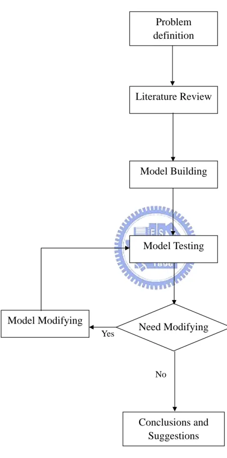
1.4 Study flowchart

There are five steps in the flowchart: 1.problem definition, 2.literature review, 3.model building, 4.model testing and modifying, 5.conclusion and suggestion. Here we represent it diagrammatically as Figure 1.1.

To begin with, we define the problem and review relative research works. Then we propose our real-time estimateion model. Finally, through analyzing the testing results, we keep modifying our model and testing the accuracy of this model.

The outline of the paper is follows. In chapter 1, the objective of this study is described. In chapter 2, reviews of papers related to this study are presented. In chapter 3, we construct and describe a real-time arrival time estimateion model. Chapter 4 describes how we test this model and shows testing results. In chapter 5, the findings of this study and suggests are summarized, including several future possible research topics.

Figure 1.1 Study Flowchart

Problem

definition

Literature Review

Model Building

Model Testing

Conclusions and

Suggestions

Model Modifying

Need Modifying

Chapter 2 Literature Review

In this chapter, we review papers related to travel time estimateion methods. Section 2.1 includes papers in corresponding with estimateion travel time on highway, while Section 2.2 is about that in urban area. Section 2.3 summarizes these reviews and makes a conclusion.

2.1 Review of the Literatures relating to estimateion travel

time on highway

Most of the papers about travel time estimateion on highway are based on traffic flow theory and artificial neural network to estimate travel time.

Jasperse, Peterson, and Yamance use flow theory to estimate vehicle travel time, while Lee and Rong use artificial neural network. Concepts of these estimateion methods are explained as follows.

In order to provide drivers with useful and correct information, Jasperse [2] develop algorithms to calculate travel time and queue-length. Main source of the input data is from loop detector (vehicle speed and traffic flow). The algorithms are proved useful by comparing the outcome of the algorithms with real data recorded by another system. Also the algorithms will be briefly outlined. The findings are that in the common cases (short and long-closed road-segments ) the estimation of travel time is satisfactory. The queue-length estimator for long closed road-segments seems also adequate. The algorithms doesn’t function for open-long segments and with large absences of the input data.

travel time. The proposed algorithms has the ability to be used in any traffic situation between two points. It also has the ability account for relative speeds and densities of vehicles within the traffic stream. Calibration and field testing of the new algorithm of has indicated that substantial improvements in travel time estimateion can be achieved when compare to existing system currently operational in Melbourne, Australia.

Yamance [4] develop the Travel Time Estimation System to estimate the travel tome using the data of Automatic Vehicle Identification (AVI) and ultrasonic vehicle detectors (UVDs). This system collects technique and estimates travel time for 106 major sections, taking account of data from UVDs. The key technology of the system is being able to estimate travel time accurately in various traffic situations. They develop a new algorithm for travel time estimation. In the algorithm, if the estimated travel time is considerably long, drivers may experience delays in receiving travel time information that may lead to incongruities with actual travel time. Therefore, they develop two more methods to overcome this problem.

Lee [7] uses artificial neural networks to build a travel time forecasting model. The input data is the real time traffic information. The traffic information involves the GPS data of bus, the data of vehicle detector and the data of incident. The section of highway in this research is from Xi-luo to Yong-kang interchange. It was divided into several segments for model building. The effects of four separating ways to the travel time forecasting are discussed fewer data sources. This study showed very promising practical applicability of the proposed models in the Intelligent Transportation System ( ITS) context.

traffic information in first phase. Second, he uses artificial neural network with three layers, fully connected and feed-forward, and backpropagation algorithm to build forecasting highway travel time models. Using simulation to produce the relative data of traffic character detected by vehicle detector sequentially for the base of artificial neural network training and testing. The result of this research can be provided to forecast travel time in real time highway travel time estimation.

2.2 Review of the Literatures relating to estimateion travel

time on urban area

Most of the papers about travel time estimateion in urban area are based on traffic flow theory and mathematics models to estimate travel time.

Sanghoon uses flow theory to estimate vehicle travel time, while Chang and Wu used mathematics algorithm. Concepts of these estimateion methods are as follows.

Sanghoon Bae [10] uses Automatic Vehicle Location (AVL) system equipped buses as probe vehicles to estimate bus travel time. Since many transit organizations throughout the North America are currently operating these AVL buses on their bus routes, in a sense, existing AVL bus would be the most cost-effective probe vehicle that can be utilized for data collection in the proactive mode. The initial objective for the first goal was to model and simulate the dynamic bus behaviors at a single and multiple buses using time varying passenger arrival rate and passenger boarding rate. Then, a prototype arrival time estimation model is simulated by adopting the

Parameter Adaptation Algorithm (real-time identification). Later in the research, a dynamic link travel time function was developed by dividing the conventional arterial

link into two regions.

Kuo [15] divided the estimateion model for bus arrival time into the long-term and short-term models by time lag to fulfill the different demand of passengers. In the building of long-term model, this paper applies dynamic and stochastic travel time to calculate the expectation and variance of link travel time and uses Fast Fourier Transform (FFT) to obtain the function types. In the other hand, this study proposes three short-term estimateion models and evaluates them by precision, robustness and stability After model building, this study finds that the point of demarcation of long term and short-term estimateion models is 35 minute. In validation, it discusses the estimateion error with respect to route distance, time lag and intersections. At last, this study also validates the model precision on the multi-route through reality investigation.

Wu [8] used GPS positioning information to estimate vehicle travel time. In this research mainly using vehicle historical travel information to estimate vehicle travel time. In order to make the estimation module to fit both the interurban and urban trips, he divided the vehicle travel time into vehicle running time and vehicle delay time. At the same time, in order to amend the shortcoming that it could not response the sudden change of vehicle running pattern of using historical travel information to estimate vehicle travel time. He use the GPS positioning information, includes vehicle average running speed and former vehicle travel time information to adjust the vehicle running time estimation. And he used the vehicle real stopping behavior to adjust the vehicle delay time estimation.

link. However the buses have their main missions to do, such as carrying passengers, we must filter out the unneeded data to provide accurate travel information. The data processing model includes two parts. One is the data filtering model to filter out the un-normal low speeds resulted from stops for collecting passengers or red light. The other is the data-cutting model. This model using the change point analysis of statistic theory to find a cutting point where the data has significant difference. The result showed that the data filtering model and the data-cutting model could work well.

2.3 Summary

1. I this study, we choose to focus our research on travel time estimation in urban area. The reason is that, although we found that most papers are mainly written for that on highway but rarely for urban area, the

importance of urban area travel time estimation in APTS, however, is still none the less.

2. This study takes GPS as its main data source for the sake of cost and labor. A majority of papers are based on traffic flow theory and artificial neural network. But through those methods, we have to install a lot of detectors in urban area, and that costs much.

3. Former researches have done well in processing travel time and historical vehicle speed data. So, by using those reviewed results, this paper is intended as a further research in waiting time estimateion, hoping for estimateing bus traveling time more accurately.

Chapter 3 Model Building

This section explains principles of the estimation model. We divide the bus travel time into two categories: “bus running time” and “bus delay time”. The former refers to the total sum of running time in each sub-section, and the latter means the total sum of the waiting time at each intersection. Concepts of the estimation model are

explained in section 3.1.

In this study, we take GPS as the major data source. Thus, before we start to construct our model, we should preprocess these data, build databases for historical average speed and predecessor bus speed to meet the needs of this model. The processing of bus speed data is explained in section 3.2.

By using average speed, we are able to estimate the running time. When the traffic status is normal, we use the historical bus average running speed to estimate running time. And when the traffic status is abnormal, we switch to front platoon’s speed data to estimate running time. The concept of running time estimation is explained in section 3.3.

The bus delay time is divided into two parts: the first part is the time for vehicles waiting for traffic signals; the second part is the time for passengers boarding on buses. In this study, we even divide the first part into “the time waiting for red light” and “the time waiting for the front platoon dismissing”. The details will be explained in section 3.4.

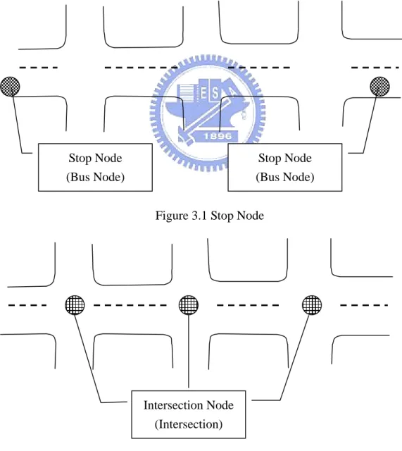
First, we have to define the most elementary concepts here: links and nodes. Both of them have two kinds individually: link and sub-link, stop node and intersection node, and each of them is described as follows:

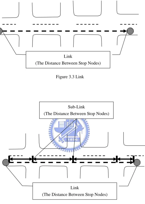
A stop node refers to the point where the bus stop is placed (Figure 3.1), and a intersection node refers to where the intersection is. (Figure 3.2) A link means the segment between two stop nodes (Figure 3.3), while the sub-link means the distance between an intersection node or a bus node and another intersection node (Figure 3.4).

Figure 3.1 Stop Node

Figure 3.2 Intersection Node Stop Node (Bus Node) Stop Node (Bus Node) Intersection Node (Intersection)

Figure 3.3 Link

Figure 3.4 Sub-Link

In this study, bus travel time is divided into bus running time and bus waiting time. The former means the total sum of the running time in each sub-link; the latter is the sum of the waiting time at each intersection.

Link

(The Distance Between Stop Nodes)

Link

(The Distance Between Stop Nodes) Sub-Link

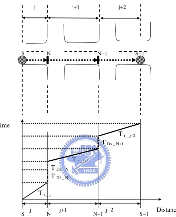
Take figure 3.5 for example, node S and node S+1 refers to bus stop nodes, and node N and node N+1 are intersection nodes. In Figure 3.5, we illustrate the bus travel time between the stop node S and the stop node S+1: the running time is the sum of the running time of sub-link j, j+1 and j+2, and the waiting time is the sum of the waiting time on intersection node N and N+1.

When the bus travels from the stop node S to the intersection node N, its travel time in the sub-link j equals to

T

intersection with red light and fleet ahead. Thus we divide the bus waiting time into two parts. The first part (the time for the bus to wait for traffic signal change) equals to

T

to

T

When the bus travels from the intersection node N to the intersection node N+1, its travel time in link j+1 equals to

T

intersection with red light but without fleet ahead, the bus waiting time is only

Figure 3.5 The Theory of Bus Travel Time Estimateion

3.2 Processing of bus speed data

Before the estimation, we must process the bus speed data in advance, in order to compute the average speed in each sub-link more precisely. For some abnormal bus speed data may affect the accuracy of the average bus running speed. There are some reasons for the occurrence of abnormal bus speed data: 1. buses have to wait for

S+1 N+1 S N N N+1 S S+1 j j+1 j+2

T

T

T

T

T

Time

Distance

T

passengers boarding at bus stops 2.wait for the red light at intersections 3.encounter congested or abnormal traffic situations ,such as accidents or rush hours.

3.2.1 Data filter model of historical bus average running speed data

We use a data filter model to filter out those abnormal data that we don’t need, to provide more accurate historical bus average running speed. Concepts of the filter model are explained as a flowchart in Figure 3.6. [9].

First, the model filters out some bus speed data whose speed value equals zero and deletes it. Also, it deletes the bus speed data by ten seconds before and after the time when the bus speed equals zero. The stop range is within a certain distance from bus stop or intersection.

Figure 3.6 Data filter model Flowchart (cited from [9])

The average bus speed in different links may vary much in one day, moreover, due to the constant changes of the average speed in different links, buses may may have higher or lower average speed in a single day. So in this study we apply

"Point-Changing Analysis" to cut the historical average speed database into different speed type time periods, preparing for estimation of waiting time or for previous bus speed database. "Point-Changing Analysis" should be constructed on the basis of the hypothesis that there is not changing point. If this hypothesis is rejected, then it means that there are changing points existing in that bus speed data. Therefore, we start to estimate to position of these points. After these positions are all found, periods with different speed data are just what we need, for example, Figure 3.7.

Figure 3.7 Data-cutting model flowchart(cited from [9])

3.2.2 Front platoon bus running speed data

When the traffic is in an abnormal situation, such as accident or congestion, the previous bus running speed data is used to compute the average speed to estimate the bus running time.

Every bus speed data closest to present time in every link is saved as the

Hypotheses testing H₀: no cutting point.

Estimate the cutting point (M aximum Likelihood Estimator)

previous bus running speed data in a database, and real-time GPS data is received to update it.

Owing that bus speed in every link changes differently with time, if the database is not updated with new data after a certain period of time, data in the database may not be able to represent present traffic situations. So, we set a restriction of time in the validity of data.

The restriction of time means whether current time passes through a different speed type time period. If it does, then the previous bus running speed database will be refreshed by latest data.

3.3 Concept of Bus running time Estimation

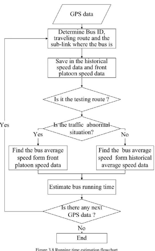
The flowcharts of bus running time estimation are explained as follows. (Figure 3.8)

Step 1: When receiving GPS data, we check the vehicle number of the data and which link it is in.

Step 2:Store the bus speed data in historical bus speed database and the previous bus speed database.

Step 3: determine whether the GPS data is from our testing traveling route or not. If yes, go to next step; else, continue to receive the coming data.

is whether the difference of vehicle speed of GPS data and historical average speed over-weights the critical value. If yes, then it is regarded as an abnormal situation.

Step 5: If it is abnormal, we obtain the bus average speed from the previous bus running speed data. Otherwise, we compute the bus average speed from the history bus average running speed data.

Step 6: This estimation model uses the bus average speed to compute the bus running time in each sub-link as equation 3.3.1.

T i _R_j = Lj / AveSpeed (j) 3.3.1

Where, T i _R_j = running time of bus i in the sub- link j i = bus number

Lj = distance of the sub- link j

3.4 Concept of Bus Waiting time Estimation

The bus delay time is divided into two parts. the first part is the time for vehicles waiting for traffic signals; the second part is the time for passengers boarding on buses. In this study, we additionally divide the first part into “the time waiting for red light” and “the time waiting for the front platoon dismissing”

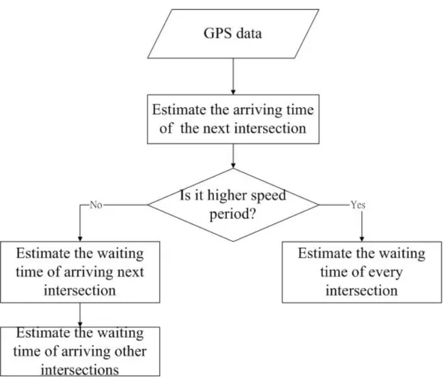
We set two situations in estimation of waiting time. The first is that, when the current time is in a higher vehicle speed time period, we determine whether the buses need to stop at every individual intersection or not, and then we estimate the waiting time. The second is that, when the current time is in a lower vehicle speed time period, we determine whether the bus has to wait at the next intersection, and waiting time is estimateed in that intersection. As for other intersections, we set an expected waiting time. Above concepts are explained in Figure 3.9.

Step 1: Receiving GPS data, the model estimates the arriving time at the next intersection. If the bus is in a sub-link, the model estimates the running time for those coming roads it hasn’t take. With the bus in the range of stop node and zero bus speed, the model sets waiting time as zero, and estimates the running time at next sub-link, to get the arriving time at the next intersection. But if the bus is in the range of intersection node and is at zero speed, the model estimates waiting time by current time; if the speed is not zero, then it estimates the running time in the next sub-link, to get the arriving time at next intersection.

Step 2: The model has to check whether it is now at a higher speed vehicle speed time period.

Step 3. The model set two situations in the estimation of waiting time: (1)if it is now at a higher speed time period, the model decides whether the buses will meet the red light or not, according to the time arriving at each intersection and phase planning table. If needed, then it estimates the waiting time.(2) if it is now at a lower speed time period, the model decides whether the buses has to wait at the next intersection or not. If needed, then it estimates the waiting time. For other intersections, expected waiting time is applied.

Figure 3.9 Estimation waiting time flowcharts

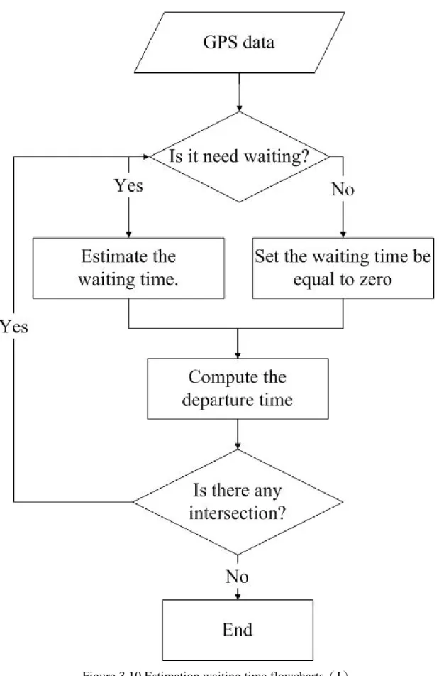
time for every intersection. The concepts will be shown illustrated as Figure 3.10.

Step 1:The model decides whether the buses encounter a red light or not, according to the arriving time at the next intersection and the phase planning table of that intersection.

Step 2:if waiting for a red light is needed, the model calculates the seconds left of the red phase. Being not needed, then the waiting time is set to be zero.

Step 3: Based on the waiting time estimated in above stops, we obtain the starting time of the bus from that intersection.

Step 4:Then the model determines if there are any intersections needing the estimation of waiting time. If yes, then we continue the estimation; else, we bring it to an end.

Figure 3.10 Estimation waiting time flowcharts（I）

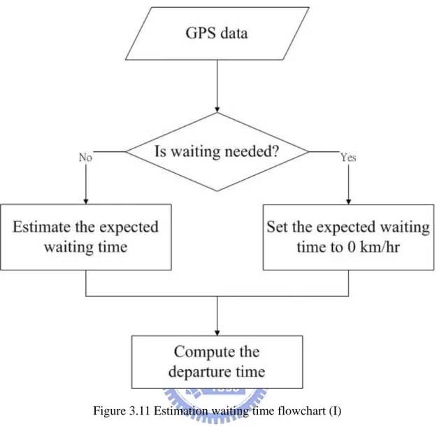
the estimation of waiting time. The first step is to estimate the waiting time at the next intersection, as the flowchart in Figure 3.11.

Step 1:The model decides whether the buses encounter a red light or not, according to the estimated arriving time at the next intersection and the phase planning table.

Step 2:if waiting for a red light is needed, the waiting time of that intersection equals to the seconds left of the red phase. Otherwise the waiting time is set to be zero.

Step 3: Based on the waiting time estimated in above stops, we obtain the starting time of the bus from that intersection.

Figure 3.11 Estimation waiting time flowchart (I)

In the second step, the model estimates the waiting time of other intersections, as Figure 3.12

Step 1: The model calculates the expected waiting probability of each

intersection. The probability equals to red phase split, the ratio that red phase over total cycle length.

Step 2: Expected waiting time is taken as the estimated waiting time of each intersection. This time is obtained by expected waiting probability multiplies

Step 3: Then the model determines if there are any intersections that need the estimation of waiting time. If yes, then we continue the estimation; else, we bring it to an end.

Chapter 4 Model Testing

This section explains the framework and result of model testing. The initial process of the model testing is explained in section 4.1. The result of the model testing is presented in section 4.2.

4.1 Initial process of Model testing

This section explains how we perform the model testing. In section 4.1.1, we define the testing targets and the reason why they are chosen. In section 4.1.2, we explain how historical data is collected and how we process it. Section 4.1.3 explains the parameter setting of this estimation model. And in section 4.1.4, the procedure of this estimation model is described.

4.1.1 Explanation of testing target

We choose the route number 106 of TaiChung City Bus as the testing target. In this route, eight bus stops are chosen as shown in Figure 4.1, and the real travel time from first stop to the eighth stop is about ten minutes.

In order to test the estimation model in different traffic flow situations, we perform our test on Wednesday evening and Saturday noon. We estimate the arrival time and travel time of buses, and then analyze the difference in the arrival time between the actual and the estimation value.

Figure 4.1 The Route 22 of Taichung City Passenger Transport

4.1.2 Processing of historical speed data

In order to compute the historical bus average speed, we have to collect enough speed data. Thus, GPS data of the testing target as long as forty-eight days has been collected for this purpose, and each data is received every twenty seconds.

Then, we filter out the unneeded data before using these GPS data to compute the historical bus average running speed, for abnormal bus speed data will greatly affect the accuracy of average running speed. Generally, abnormal bus speed data is resulted from passengers boarding, accidents, or congested traffic.

And then we compute the historical average speed of each sub-link. In order to reflect the real situation correctly, we have to choose a historical average speed that is most like the current situation. For example, if current testing time is 10:30, then

S4 S3 S2 S1 S5 S6 S7 S8 : Road : Bus Stop : Traveling Direction

we’ll choose the average speed in the period from 10:00 to 11:00 in historical speed database.

Moreover, we apply “Point-Changing Analysis” to split historical average speed data into several sections as follows: 06:00 to 12:00, Table 4.1; 12:00 to 18:00, Table 4.2; 18:00 to 24:00, Table 4.3. Since we have no GPS data from 00:00 to 06:00, we do nothing in this section.

After the analysis, we have four periods in which the bus speed is higher: 06:00 to 07:45; 09:45 to 11:30; 14:00 to 18:15, and 20:00 to 23:29. Also, three periods in which the bus speed is lower: 07:45 to 09:45; 11:30 to 14:00, and 18:15 to 20:00, as listed in Table 4.4.

Table 4.1 Result of using the change point analysis (I)

Time AvgSpeed Operation 1 Operation 2 Operation 3

06_00~06_15 32.00 Delete 06_15~06_30 28.55 Delete 06_30~06_45 23.06 Delete 06_45~07_00 25.10 Delete 07_00~07_15 22.26 Delete 07_15~07_30 21.31 Delete 07_30~07_45 22.58 Delete 07_45~08_00 23.86 Cutting-point Delete 08_00~08_15 15.01 Delete 08_15~08_30 18.57 Delete 08_30~08_45 23.64 Delete 08_45~09_00 23.01 Cutting-point Delete 09_00~09_15 19.88 Delete 09_15~09_30 26.62 Delete 09_30~09_45 23.32 Delete 09_45~10_00 22.50 Delete Cutting-point 10_00~10_15 22.66 Delete

10_15~10_30 23.09 Delete 10_30~10_45 23.12 Delete 10_45~11_00 23.83 Delete 11_00~11_15 24.32 Delete 11_15~11_30 24.58 Delete 11_30~11_45 21.66 Delete 11_45~12_00 18.91 Delete

Table 4.2 Result of using the change point analysis (II)

Time AvgSpeed Operation 1 Operation 2 Operation 3 12_00~12_15 22.07 Delete 12_15~12_30 22.24 Delete 12_30~12_45 21.47 Delete 12_45~13_00 18.91 Delete 13_00~13_15 20.96 Delete 13_15~13_30 18.20 Delete 13_30~13_45 16.81 Delete 13_45~14_00 19.26 Delete 14_00~14_15 24.93 Cutting-point 14_15~14_30 24.72 14_30~14_45 23.43 14_45/~15_00 24.31 Cutting-point Delete 15_00~15_15 24.78 Delete 15_15~15_30 24.05 Delete 15_30~15_45 24.60 Delete 15_45~16_00 23.59 Delete 16_00~16_15 23.89 Delete 16_15~16_30 22.61 Delete 16_30~16_45 23.47 Delete 16_45~17_00 21.86 Delete 17_00~17_15 22.25 Delete 17_15~17_30 22.00 Cutting-point Delete 17_30~17_45 20.91 Delete 17_45~18_00 20.50 Delete

Table 4.3 Result of using the change point analysis (III)

Time AvgSpeed Operation 1 Operation 2

18_00~18_15 20.39 Delete 18_15~18_30 20.16 Cutting-point 18_30~18_45 19.68 18_45~19_00 19.96 19_00~19_15 22.74 19_15~19_30 21.21 19_30~19_45 25.75 19_45~20_00 24.31 20_00~20_15 23.10 Cutting-point 20_15~20_30 21.91 20_30~20_45 21.41 20_45~21_00 22.23 21_00~21_15 23.21 21_15~21_30 21.08 21_30~21_45 22.60 21_45~22_00 20.20 22_00~22_15 19.67 22_15~22_30 24.19 22_30~22_45 24.54 22_45~23_00 26.31 23_00~23_15 37.75 23_15~23_30 37.33

Table 4.4 Period of different average speed type

Period Average speed Type of average speed 00_00_00~00_06_00 Null Null 00_06_00~07_45_00 24.98 Higher average speed 07_45_00~09_45_00 21.74 Lower average speed 09_45_00~11_30_00 23.44 Higher average speed 11_30_00~14_00_00 20.05 Lower average speed 14_00_00~18_15_00 23.08 Higher average speed 18_15_00~20_00_00 21.97 Lower average speed 20_00_00~23_59_59 24.68 Higher average speed

4.1.3 Parameter setting

Three parameters need be set before using this estimation model to estimate the bus travel time: the threshed speed, the stop range of filter model, and the critical value of speed error.

In setting the threshed speed, because our data is received every 20 seconds, we will have problem judging the real critical value of speed. Therefore we follow the value 15 km/hr mentioned in the previous paper.[9]

The word “stop range” refers to a certain distance from bus stop or intersection, and the criteria to set it is “the distance that covers 90% of the low speed data”. According to those collected GPS data, we re-calculate the speed of the four buses and their distance from the stop node, as listed in Table 4.5, 4.6, 4.7 and 4.8. After calculating, we found that there are 95.24% of the speed data occurred in less than 50 meters. So, we set the value to 50 meters.

Table 4.5 Stop range (Bus1)

Time Length speed

195037 15 40 195057 15 40 195117 20 0 195137 34 44 195157 34 44 195217 50 29 195237 34 31 195257 34 31 195317 15 0 195337 13 0 195357 13 0 195417 8 22

Table 4.6 Stop range (Bus2)

Time Length speed

185915 0 20 185935 0 38 185955 0 37 190015 68 18 190036 53 12 190055 34 0 190115 34 0 190135 35 0 190156 26 12 190216 20 25 190235 44 24 190256 48 40 190316 33 0 190336 33 0 190356 53 0 190416 50 9

Table 4.7 Stop range (Bus3)

Time Length speed

155932 14 14 155952 14 14 160012 14 14 160032 0 38 160052 0 0 160112 0 0 160132 0 0 160152 0 0 160212 0 25 160232 29 33 160452 12 0 160512 15 0 160532 15 0 160552 21 0 160612 17 0

Table 4.8 Stop range (Bus4)

Time Length speed

142032 19 35 142052 35 7 142112 35 7 142132 11 38 142152 5 9 142212 5 9 142232 17 35 142252 10 0 142212 10 0 142231 10 0 142252 30 0 142312 30 0 142332 33 35 142352 31 40 142412 31 40 142432 33 5 142452 30 0 142512 30 0 142532 28 0 142552 25 40 142612 0 22 142632 46 1 142652 38 38 142712 38 38 142732 46 0 142752 48 0 142812 48 0 142832 48 0

By threshed speed, we can judge whether we should use the previous bus speed or historical speed data as the current bus speed. If the differential of vehicle speed is larger than threshed speed, then it is regarded as abnormal situation, and we’ll take the

previous bus speed as the average speed of the link.

The restriction of time in the validity of data is decided by point-changing analysis, and from that, we may divide the database into different periods of speed type, as listed in Table 4.4. Therefore, when current time cover the next period, the previous bus running speed database will be refreshed.

4.1.4 Procedure of estimation model

This section explains the procedure how we estimate the bus travel time. Figure 4.2 is the flowchart that explains all these steps.

Step 1:

When receiving GPS data, we determine the vehicle number of the data and which route or sub-link the bus is in.

Step 2:

Store the speed data into historical speed database and previous car speed database.

Step 3:

Check if the bus traveling route is the testing route or not. If yes, go to next step; otherwise we continue to receive the next GPS data.

Step 4:

Apply the estimation model to estimate traveling time. At first, we check whether the differential of current speed and historical speed is in the range of threshed speed (5 km/hr). If yes, then we take historical speed data as the average speed at the link. Otherwise, we take the previous speed data. In this way, running time can be derived from the distance of sub-links divided by average speed.

Step 5:

The model determines which period in the historical database the current time is in. If it is in the period of higher speed, .our model will judge whether the bus has to wait for a red light or not, according to the arrival time and the phase planning table. Also, we will computer the needed waiting time.

If it is in the period of lower speed, the model will merely judge if the bus has to wait at the next intersection. If the signal turns red, then we calculate the waiting time and set expected waiting time to other intersections.

Step 6:

The travel time is set as the total sum of the running time and the waiting time..

Step 7:

By adding the next travel time to current time, we get the time when the buses reach the next stop. Thus the time buses reach every bus stops is obtained.

4.2 Result of model testing

We choose the route 106 of TaiChung City Bus as the testing target. The testing time was on May 28, 2003 and May 31, 2003. We performed these tests on four different buses.

4.2.1 Analysis method

The accuracy of this estimation result is analyzed in this section. Several parameters are also computed out: the average error of the estimation waiting time, the error and the maximum error at each stop, the average absolute error and the percentage of average absolute error of estimation travel time. Finally, we perform a goodness-of –fit test of the estimation travel time at each link.

The error of estimated arrival time at every stop node is equal to the value that the actual arrival time subtracts the estimation arrival time, as shown in equation 4.2.

The maximum error of arrival time at every stop is equal to the maximum value of estimated arrival time errors, as shown in equation 4.3.

Es = Ps - As 4.2

Max (Es) =Max (︱ Ps – As︱ ) 4.3

Where, Es = the error of this estimation arrival time at sth stop.

Max(Es) = the maximum error of this estimation arrival time at sth stop. As = the actual arrival time at sth stop.

Ps = the estimation arrival time at sth stop. s = stop number

The average error of the estimated waiting time equals to the total sum of the value that the actual waiting time subtract the estimation waiting time and divided by the number of data, as equation 4.3

Where, E w = the average error of the estimation waiting time..

Ni = the number of data.

A w = the actual waiting time.

P w = the estimation waiting time.

The average absolute error is constructed to understand the difference between the estimated travel time and the real travel time, as shown in the equation 4.4.

ΣP w – A w

E w= 4.1

Where, E mean = the average modulus error.

Ni = the number of data.

A t = the actual travel time.

P t = the estimation travel time.

We compute the percentage of average absolute error of estimation travel time as another estimation index, because the value involved in absolute error could not give out the comprehensive evaluation of our test.

Where, E percentage = the percentage of average modulus error of estimation travel

time

A t = the actual travel time.

P t = the estimation travel time.

Ni = the number of data

We perform the goodness-of -fit-test that could determine whether the error is in acceptable range or not as shown in the equation 4.5.

Σ︱P t – A t︱ E mean= 4.4 Ni ︱P t –A t︱ A t E percentage= 4.5 Ni Σ

The degree of freedom (v) is equal to (k-1).

Where, Oi = the observation value, the estimation travel time.

е

4.2.2 Result analyzing

1. Error of arrival time

We performed these tests on two different buses and in the period of lower speed when the traffic is congested. If the error value is positive, then it means that we over-estimate the arrival time. Otherwise, it means that we under-estimate. The results of the errors computed are as illustrated in Table 4-9 and Table 4-10(Figure 4.3 and Figure 4.4).

From these results, we can find that the errors of the estimated arrival time are roughly about 30 seconds, and the maximum one is 33 seconds. We may say that in this case, it performs well in arrival time estimation.

χ2 =

Σ

е

е

Table 4-9 Error of arrival time (bus 1) Bus stop From 19:48:50 To 19:57:43; Wednesday

(Error of this estimation arrival time: second)

stop1 70 70 86 0 0 0 0 0 0 0 stop2 46 46 49 -24 0 0 0 0 0 0 stop3 -6 -6 28 -76 -53 -53 0 0 0 0 stop4 24 24 36 -46 -23 -23 0 0 0 0 stop5 32 32 77 -38 -15 -15 -4 -4 0 0 stop6 30 30 53 -40 -17 -17 -6 -6 -2 0 stop7 -4 0 50 -62 -47 -51 -36 -36 -24 0 stop8 -67 -63 -13 -65 -50 -54 -39 -39 -27 -33 -100 -80 -60 -40 -20 0 20 40 60 80 100

stop1 stop2 stop3 stop4 stop5 stop6 stop7 stop8

Table 4-10 Error of arrival time (bus 2) Bus

stop

From 18:59:25 To 19:11:20

(Error of this estimation arrival time: second)

Stop1 _{-1 -3} Stop2 _{-7 -9 1 -13} Stop3 _{-44 -46 -33 -47 -42 -17 -17 -17 -17} Stop4 _{-50 -75 -76 -90 -105 -60 -60 -60 -60} Stop5 _{-111 -113 -94 -108 -123 -78 -78 -78 -78 -18} Stop6 _{-124 -126 -107 -121 -136 -91 -91 -91 -91 -31 -13 -13 -13 -13 -13} Stop7 _{-151 -156 -136 -150 -165 -120 -120 -120 -120 -60 -42 -42 -42 -42 -42} Stop8 _{-60 -80 -56 -70 -85 -40 -40 -40 -40 -40 -22 -22 -22 -22 -22 -22 -19 -19} -180 -160 -140 -120 -100 -80 -60 -40 -20 0 20

stop1 stop2 stop3 stop4 stop5 stop6 stop7 stop8

Figure 4.4 Error of arrival time (bus 2)

speed when the traffic is not congested. If the error value is positive, then it means that we over-estimate the arrival time. Otherwise, it means that we under-estimate. The results of the errors computed are as illustrated in Table 4-11 and Table

4-12(Figure 4.5 and Figure 4.5).

From these results, we can find that the errors of the estimated arrival time are roughly about 30 seconds, and the maximum one is 34 seconds. We may say that in this case, it performs well in arrival time estimation.

Table 4-11 Error of arrival time (bus 3)

Bus stop

From 14:20:15 To 14:29:41

(Error of this estimation arrival time: second) Stop1 -34 11 11 1 1 Stop2 -78 -13 -13 -27 -27 -28 -4 Stop3 -61 43 43 28 28 27 51 30 Stop4 -107 15 15 -3 -3 -4 20 -1 -31 -31 Stop5 -134 25 25 5 5 4 8 7 -23 -23 Stop6 -93 80 80 60 60 59 63 66 32 32 25 25 Stop7 -107 96 96 69 69 64 68 67 33 33 26 26 Stop8 -106 99 99 70 70 65 69 68 64 64 57 57 31 31

-150 -100 -50 0 50 100 150

stop1 stop2 stop3 stop4 stop5 stop6 stop7 stop8

Figure 4.5 Error of arrival time (bus 3)

Table 4-12 Error of arrival time (bus 4) Bus stop From 15:59:01 To 16:06:05

(error of this estimation arrival time: second) Stop1 -56 Stop2 -37 19 18 18 12 Stop3 -44 12 9 9 1 12 12 Stop4 -4 52 45 45 38 25 25 Stop5 -3 53 45 45 36 23 23 2 Stop6 16 72 64 64 55 42 42 17 Stop7 18 77 64 64 51 38 38 13 4 4 Stop8 9 68 55 55 42 29 29 4 5 5 9 9 5

-80 -60 -40 -20 0 20 40 60 80 100

stop1 stop2 stop3 stop4 stop5 stop6 stop7 stop8

Figure 4.6 Error of arrival time (bus 4)

2. Average error of the estimation waiting time

In order to analyze the error of the estimated waiting time, we perform the test on four different buses to compute the average error of the estimation waiting time. If the error value is positive, then it means that we over-estimate the arrival time. Otherwise, it means that we under-estimate. The results of the errors computed are as illustrated in Table 4-13.

From these results, we can find that the errors of the estimated arrival time are roughly about 20 seconds, and the maximum one is 36 seconds. We may say that in this case, it performs well in arrival time estimation.

We analyze the results and find that, the error under lower speed situation is greater, and can even be as large as 36 seconds. There are two reasons to be so. First, the estimation model is constructed in higher speed situation, therefore if the police

manually adjust the phase planning table, a larger error will therewith occur. Moreover, since the error enlarges as the previous error, intersections in the end of the route will be affected more.

Table 4-13 Average error of the estimation waiting time

Bus stop Bus 1 (second) Bus 2 (second) Bus 3 (second) Bus 4 (second) stop1 51.000 36.000 43.000 98.000 stop2 29.000 35.250 28.000 25.000 stop3 3.800 11.800 6.000 6.000 stop4 -8.333 -5.000 14.667 14.778 stop5 -16.00 -14.000 13.000 11.200 stop6 -0.545 13.636 24.545 22.364 stop7 -11.000 -13.000 10.000 10.400 stop8 -11.389 -7.277 11.556 3.500

3. Percentage of average absolute error of estimation travel time

In order to analyze the error of the estimated travel time, we perform the test on four different buses to compute the average absolute error of estimated travel time and average absolute error percentage. The results of the errors computed are as illustrated in Table 4-14.

From these results, we can find that the average absolute errors of the estimated travel time are all within 15 seconds, and the maximum one is 14 seconds. The average absolute error percentage is roughly less than 30%, and the maximum one is 93% We may say that in this case, it performs well in travel time estimation.

According to the results, we analyze and find that although we have only 12 seconds in average absolute error, but the average error percentage is as high as 93%.

This is mainly because that the travel time in that route is as short as 15 seconds, so that the percentage is also higher.

Table 4-14 Average absolute error of estimation travel time Number of Sub-link Average modulus error Percentage of average

modulus error (%) Link 1 _{38.22222 16.74738} Link 2 40.1 75.23565 Link 3 98.1 181.5063 Link 4 91.33333 172.7671 Link 5 24.94444 77.98737 Link 6 45 101.0223 Link 7 33.1 117.2838 Link 8 64.05 46.57097

4. Goodness-of –fit test

We perform the goodness-of -fit-test to test if the error of estimated travel time and actual travel time falls in acceptable range or not. We take four buses to take to test, and the results are shown in table 4-15.

According to the results, after the test, all the estimated travel time in eight routes all fall in an acceptable range.

Table 4-15 Goodness-of -fit-test

Number of Sub-link χ2 χ2 (0.95, 7) Link 1 _{3.609 14.07} Link 2 5.003 14.07 Link 3 12.410 14.07 Link 4 8.877 14.07 Link 5 2.315 14.07 Link 6 14.05 14.07 Link 7 9.218 14.07 Link 8 1.629 14.07

4.3 Summary

According to the results of the model testing in section 4.2, we draw some conclusions as follows:

1. Whether in periods of higher speed or lower speed, the error of estimation travel time is about 30 seconds, and that falls in an acceptable range.

2. Whether in periods of higher speed or lower speed, the error of estimation waiting time is about 15 seconds, and that falls in an acceptable range.

3. The model may over-estimate or under-estimate the waiting time and sometimes a large error may occur. The reason is that the police manually adjusts the phase planning table, thus makes the error occur.

4. When the travel time in the route is shorter, we may obtain higher error percentage in estimation of travel time in that route.

Chapter 5 Conclusions and Suggestions

In this section, we make conclusions and suggestions about this research. Section 5.1 and 5.2 discuss on conclusions and suggestions, respectively.

5.1 Conclusions

1. Whether in high or low speed period, the errors of travel time estimation and waiting time estimation usually fall in an acceptable range. Therefore, we may say that we have a good estimation result.

2. We may overestimate or underestimate the waiting time of the next intersection, mainly because of the traffic control performed there by the police during peak hours or estimation errors in the present intersection. In this way, owing to the errors, we may have a bigger error in the following intersections.

3. In some intersections where travel time is shorter, the average absolute error percentage will be higher, but the average error value is still in an acceptable range.

4. Through the analysis method of changing points, we divide the historical average speed database into some different categories by its vehicle speed. Then we found that it matches the real situations, and can surely improve the model’s domination on them.

5.2 Suggestions

In this section, we make some suggestions for future researches as follows: 1. This study didn’t leave a mark on boarding time, but due to its importance,

2. Not encountering abnormal situations, so that we didn’t have a chance to test the model in estimateing the travel time in that situation. And we also suggest future researches do some further research on it.

3. Random adjusting of signal timings in intersections makes the errors worse. Thus, it is recommended to have a further research on it in the future.

4. The transmitting frequency of GPS data effects greatly in estimateing travel time: the errors varies worse as the frequency becomes lower. So, we suggest that future researches think more on it.

Reference

[1] Sen, A., Thakuriah, P.V., Zhu X. Q., and Karr A.. (1997). “Frequency of Probe Reports and Variance of Travel Time Estimates.”, Journal of Transportation

Engineering, 123 (4), 290-297.

[2] Jasperse, Diana, van Toorenburg, Jaap, “Real-Time Estimation of Travel- Time and Queue-Lengths – A Practice Study”, Presented at 6th World Congress on Intelligent Transport Systems 1999. Toronto, Canada.

[3] Rosc, Geoff, Paterson, Darryn, “Dynamic Travel Time Estimation on Instrumented Freeways”, Presented at 6th World Congress on Intelligent Transport Systems 1999. Toronto, Canada.

[4] Yamane, Ken’ichiro, Sano, Yutaka, Furuta, Masataka, Fushiki, Takumi, “Development of Travel Time Estimation System Combining License Plat Recognition AVI and Ultrasonic Vehicle Detectors”, Presented at 6th World Congress on Intelligent Transport Systems 1999. Toronto, Canada.

[5] Bruce R. Hellinga, Liping Fu, “Reducing bias in probe-based arterial link travel time estimates”, Transportation Research-C, No.10, pp 257-273, 2002.

[6] Ashish Sen, Piyushimita (Vonu) Thakuriah, Xia-Quon Zhu, Alan Karr, “Variances of link travel time estimates: implications for optimal routes”,

International Transportations in Operational Research, No.6, pp 75-87,1999.

[7] Ying Lee, “Development of freeway bus travel time forecasting model using artificial neural networks”, master thesis, Department of Transportation and Communication Management Science of National Cheng Kung University, 2001. [8] Chia-Feng Wu, “The study of Vehicle Travel Time Estimation with GPS

Information provided”, master thesis, Department of Engineering in Traffic and Transportation of National Chiao Tung University, June 2001.

[9] Hui-Wen Chang, “The study of Usung GPS data of Buses to Estimate the Average Speed in a Link”, master thesis, Department of Engineering in Traffic and Transportation of National Chiao Tung University, June 2002.

[10] Sanghoon Bae, “Dynamic Estimation of Travel Time on Arterial Roads Using Automatic Vehicle Location (AVL) Bus as a Vehicle Probe”, Philosophy in Civil

Engineering, May 1995.

[11] Chi-Bang Chen, “Dynamic Estimation of Travel Time and Origin-Destination Demand on Freeway Corridor”, master thesis, Department of Transportation Management of Tamkang University, June 2002.

[12] Shih-Chieh Lin, ”The study of freeway bus travel time forecasting model using artificial neural networks”, master thesis, Department of Transportation and

Communication Management Science of National Cheng Kung University, 2001. [13] Chang Shiou Rong, “The study of freeway bus travel time”, master thesis, Department of Civil Engineering of National Central University, June 2000. [15] Chung-Tien Kuo, “A Estimateion Model for Bus Arrival Time and Multi-Route”,

master thesis, Department of Civil Engineering of National Taiwan University, June 2003.

[16] Matthew P.D’Angelo, Haitham M.Al-Deek , Morgan C.Wang, ”Travel Time Estimateion for Freeway Corridors”, Transportation Research Record 1676, pp 99-1073.

[17] Scot.t Swashburn, Nancy L.Nihan, ”Estimating Link Travel Time with the Mobilizer Video Image Tracking System”, Journal of Transportation Engineering. 1999.Jan.Feb. [18] Benjamin Coifman, ”Vehicle Re-Identification (VRI) and Travel Time Measurement (TTM) in Real-Time on Freeways Using Existing Loop Detector Infrastructure”, TRR1643, pp.181-191.

[19] Messer C.J. Dudek C.L and Friebele J.D, ”Method For Estimateing Travel Time and other Operational Measures in Real Time During Freeway Incident Conditions ”, HRR461, pp.1-16, 1973.

[20] Carlos. Daganzo, “Properties Of Link Travel Time Functions Under Dynamic Loads ”,

Transportation Research-B, Vol. 29 B, No. 2, pp.95-98, 1995.

[21] Benjamin Coifman, Michael Cassidy, “Vehicle reidentification and travel time measurement on congested freeways”, Transportation Research-A, Vol.36 A, No 36, pp

899-917, 2002.

[22] Benjamin Coifman, “Estimating Travel Times and Vehicle Trajectories on Freeways Using Dual Loop Detectors”, Transportation Research-A, Vol.36 A, No 36, pp. 351-364, 2002.

[23] Bruce R. Hellinga, Liping Fu,”Reducing Bias in Probe-Based Arterial Link Travel Time Estimates”, Transportation Research-C, Vol.10 A, No 10, pp. 257-273, 2002.

[24] Karlf. Petty, “Accurate Estimation of Travel Times From Single-Loop Detectors”,