國 立 交 通 大 學
交通運輸研究所
博士論文
No.063
以先進細胞自動機模式探索高速公路
時空交通特性
Exploration of Freeway Spatiotemporal
Traffic Features with Advanced Cellular
Automaton Modeling
指導教授: 藍武王博士
邱裕鈞博士
研
究 生:
許志誠
以先進細胞自動機模式探索高速公路時空交通特性
Exploration of Freeway Spatiotemporal Traffic Features with
Advanced Cellular Automaton Modeling
研 究 生: 許志誠 Student: Chih-Cheng Hsu
指導教授: 藍武王 博士 Advisors: Dr. Lawrence W. Lan
邱裕鈞 博士 Dr. Yu-Chiun Chiou
國 立 交 通 大 學
交 通 運 輸 研 究 所
博 士 論 文
A Dissertation
Submitted to Institute of Traffic and Transportation
College of Management National Chiao Tung University in Partial Fulfillment of the Requirements
for the Degree of Doctor of Philosophy in
以先進細胞自動機模式探索高速公路時空交通特性
學 生:許志誠 指導教授: 藍武王 博士
邱裕鈞 博士
國立交通大學交通運輸研究所
摘要
1992 年 物 理 學 家 Nagel 及 Schreckenberg 兩 人 首 度 將 細 胞 自 動 機 (Cellular Automaton,CA)應用於公路車流行為研究,透過幾個簡單的加減速規則,利用電腦快 速運算,讓車輛進行彼此交互作用與規則疊代,呈現出與實測相當之巨觀車流特性, 又能描述微觀車流特性。迄今已有相當數量之改良CA 模式,惟多針對小客車為研究 對象,且對細胞單元之定義均相當粗糙,亦未探討異質(指同類型車種可具不同之速 率、加減速、變換車道行為)混合(指同一道路空間可同時運行不同類型車種,如機車、 小型車、大型車)車流課題。為更符合實際車流現象,本研究發展精緻型 CA 模式,並 改良傳統CA 模式加減速過大之不合理現象,用以探索異質混合車流之時空交通特性。 本研究首先提出一個基礎的異質混合車流細胞自動機模式,該模式比以往細胞自 動機模式研究更為精細的「細胞」及「網格」概念,定義「基本單元」(CU)作為衡量 車輛及道路空間之共通單位。並進一步以時空網格被車輛細胞移動軌跡所佔用之比例 代表佔有率,以車輛細胞每個時階移動的格位數代表速率,每個時階通過的細胞數代 表流量,定義一般化佔有率、速率與流量,以精確描述異質混合車流車輛的總體行為。 經發展CA 基本模式,模擬不同車流密度情況下純車流之時空交通特性,再構建總體 交通流量、速率與佔有率的基本關係。惟模擬結果顯示車輛運行過程車速會驟降停止 之情形,模式規則待改進。 接著本研究針對前述規則之缺點提出一個修正CA 模式,該模式進一步整合駕駛 跟車空間預期效應、採取速度相依之隨機項、啟動延遲規則、變換車道與大小車互動 規則等。模擬環境設定在二車道的高速公路中進行,模擬情境為在車流中加入慢速車 (如同慢速移動瓶頸)與停止車(如同固定地點瓶頸),探討混合車流之時空交通特性,並 進一步探討車流軌跡、流量密度關係與時空車流型態。模擬結果顯示修正CA 模式能 夠呈現出真實交通環境重要的車流特性與型態。
研究最後針對模擬過程中以往CA 模式均未處理之缺點,即車輛在接近前方為停 止車輛或固定物時所出現不合理急煞車之情形,提出一個更精緻的CA 模式來改善。 模式在規則中引入Forbes 的跟車概念,利用多段線性速率修正傳統 CA 模式加減速過 大之不合理現象。經高速公路之驗證與測試發現,確能改正車輛速率驟降之缺失,並 能顯示Kerner 所提出的三相交通現象及其相變。本研究進一步利用此修正 CA 模式應 用在施工區,探討不同速率控制策略對行車效率及安全之影響。 關鍵字:異質車流、混合車流、細胞自動機、時空交通特性、高速公路
Exploration of Freeway Spatiotemporal Traffic Features
with Advanced Cellular Automaton Modeling
Student: Chih-Cheng Hsu Advisors: Dr. Lawrence W. Lan
Dr. Yu-Chiun Chiou
Institute of Traffic and Transportation
National Chiao Tung University
Abstract
Cellular automata (CA) model was first proposed by Nagel and Schreckenberg in 1992 to simulate the highway traffic. The core logic was to introduce several simple update rules for vehicle movement in computer programs to efficiently simulate the complicated interactive traffic behaviors. A considerable number of revised or extended CA models have been developed to date, most of which only focused on pure traffic with coarse cell units in the simulations. Very little has devoted to the heterogeneous traffic situations and/or mixed traffic contexts, which comprise different types of vehicle. This research aims to develop advanced CA models to simulate the spatiotemporal behaviors under heterogeneous mixed traffic contexts on freeway.
Firstly, a basic CA model is developed to explore the fundamental traffic features. Generalized definitions of traffic variables, in spatiotemporal sense, and a new concept of common unit (CU) for gauging non-identical vehicle sizes and various lane widths are presented. Pure light vehicle and pure heavy vehicle experiments are tested on a two-lane freeway context. Vehicular trajectories, flow-occupancy diagrams, and spatiotemporal traffic patterns under deterministic and stochastic conditions are displayed. The results show that abrupt speed drops occasionally emerge during the simulations.
To resolve this shortcoming, this study continues to propose a revised CA model, which considers the anticipation effect, velocity-dependent randomization, slow-to-start, lane change, and interaction among vehicles. The effects of both stationary and slow-moving bottlenecks on global traffic are examined using this revised CA model. Vehicular trajectories, flow-occupancy, and spatiotemporal traffic patterns are displayed. The results reveal noticeable traffic patterns with free flow, wide moving jam and synchronized flow phases, suggesting that the revised CA model is capable of capturing the essential features of traffic flows.
Finally, this study further proposes a refined CA model using the rationale of Forbes’ car-following concept with a piecewise-linear movement mechanism, which aims to rectify the common defect of abrupt deceleration existent in most conventional CA models. The proposed CA model is validated in a two-lane freeway mainline context. It shows that this refined CA model can fix the unrealistic deceleration behaviors, thus can reflect the genuine driver behaviors in real world. The model is also capable of revealing Kerner’s three-phase traffic patterns and phase transitions among them. Furthermore, the refined CA model is applied to simulate a highway work zone wherein traffic efficiency (maximum flow rates) and safety (speed deviations) impacted by various control schemes are investigated.
Keywords: Heterogeneous Traffic, Mixed Traffic, Cellular Automata, Spatiotemporal
誌謝
回顧這段帶職攻讀博士的歷程,真的就像一場長跑!鳴槍起跑充滿動力的衝出 去,很快的完成修課、通過資格考,並同時進行著研究,原以為順利然而事實上挑戰 才開始。研究過程不斷發現問題與找尋解決方法,加上繁重的工作負荷,經常在5 天 忙碌的工作後,週六日接著到學校研究室做研究,那就像是跑步停下來還沒喘完,又 要接著再跑的感覺。終於堅持跑完全程得以畢業,接受太多的幫助,要感謝的人實在 太多。 首先感謝我的指導教授 藍武王老師及邱裕鈞老師。感謝您們悉心、耐心的指導, 師恩浩瀚,無盡感恩。跟隨老師研究的過程,老師追求卓越的研究精神,以及嚴謹務 實的態度,是我需要持續提升與學習的地方。藍老師總是用最清楚的觀念傳授知識, 用以身作則嚴以律己的態度教育治學,得以投入師門學習我受益甚深。邱老師在研究 過程不斷在知識、課題、方法、資料與遭遇問題等給予細心的指導與幫助,使論文得 以順利完成,敬表由衷謝忱。感謝藍老師及邱老師的包容與體諒,容忍我緩慢的研究 與期刊投稿進度,並帶領我走過這一段歷程。感謝口試委員陳惠國教授、胡大瀛教授、 曾平毅教授、汪進財教授與許鉅秉教授,因為您們的指導與斧正,讓我的論文更臻嚴 謹完善。感謝所上的各位師長許鉅秉所長、汪進財教授、黃台生教授、黃承傳教授、 徐淵靜教授、馮正民教授與陳穆臻教授,求學過程渥蒙您們的諄諄教誨與指導,讓我 在學習與研究的過程,擁有更多專業知識與啟發。 感謝林局長重昌的提攜,並且讓我在最後關頭得以全心投入完成學業。感謝好友、 學長姐與學弟妹許多協助。感謝滈善(Gary)全力投入協助開發模擬程式,沒有您的幫 忙論文無法完成。感謝戰友日新學長,研究成果得以被國際期刊快速接受,歸功於您, 研究室共同奮鬥的日子,將是我難忘的回憶。感謝瓊文師母的指導讓我很快能進入CA 的研究領域,感謝仁傑學弟的加入,發展出新的研究方向與成果。感謝杰炤、益三、 豐裕學長修業期間的照顧,特別感謝易詩總是給我最及時的幫助。感謝孟佑、世昌、 彥蘅、承憲、沛儒、國洲、昭弘、永祥、群明、文斌、魏瑜、士軒、姿慧與彥斐等修 業期間的研討與協助。 感謝摯愛的家人,他們是背後支持我完成學業最大的力量。最要感謝是愛妻嘉瑜, 公務之餘還承擔所有家務及女兒的教養工作,看著女兒平安快樂成長,我滿心感激, 也讓我在修業期間得以無後顧之憂的完成學業。感謝女兒馨云總在我感覺壓力繁重之 際,給我貼心的擁抱,心裡總會湧起一股暖流。感謝爸媽養我育我,還有岳父母、大 哥、大嫂、二哥一直以來對我的支持與鼓勵,我要將這篇論文獻給摯愛的您。 志誠 謹誌 2010.8TABLE OF CONTENTS
中文摘要 ... III ABSTRACT ... V CHAPTER 1 INTRODUCTION ... 1 1.1BACKGROUND ... 1 1.2MOTIVATION ... 3 1.3RESEARCH OBJECTIVES ... 4 1.4CHAPTERS ORGANIZATION ... 5CHAPTER 2 LITERATURE REVIEW ... 7
2.1MACROSCOPIC APPROACHES ... 7
2.2MICROSCOPIC APPROACHES ... 11
2.3RELATED CA APPROACHES ... 16
2.4SUMMARY ... 22
CHAPTER 3 DEFINITIONS... 23
3.1COMMON UNIT FOR CELLS AND SITES ... 23
3.2GLOBAL TRAFFIC VARIABLES ... 24
3.3LOCAL TRAFFIC VARIABLES ... 29
3.4SIMULATION SETTING ... 30
3.5SUMMARY ... 31
CHAPTER 4 BASIC CELLULAR AUTOMATON MODEL ... 32
4.1FORWARD RULES ... 33
4.2LANE-CHANGING RULES ... 34
4.3FRAMEWORK ... 37
4.4PURE TRAFFIC SIMULATION RESULTS ... 37
4.5SUMMARY ... 46
CHAPTER 5 REVISED CELLULAR AUTOMATON MODEL ... 47
5.1MODIFICATION ... 47
5.2VALIDATION ... 50
6.3APPLICATION ... 73
6.4TRAFFIC FEATURE EXPLORATIONS ... 79
6.5SUMMARY ... 85
CHAPTER 7 CONCLUSIONS AND RECOMMENDATIONS ... 86
7.1CONCLUSIONS ... 86
7.2RECOMMENDATIONS ... 87
REFERENCES ... 88
APPENDIX ... 94
LIST OF FIGURES
FIGURE1-1RESEARCH FRAMEWORK. ... 6 FIGURE2-1AN ILLUSTRATION FOR THE ROAD SECTION WITH TWO OBSERVING STATIONS. 8 FIGURE2-2THE THEORETICAL FUNDAMENTAL DIAGRAM. ... 10 FIGURE2-3REPRESENTATION OF A SHOCK WAVE IN SPACE AND IN THE FUNDAMENTAL
DIAGRAM. ... 10 FIGURE2-4COMPARISON THE HOMOGENEOUS AND INHOMOGENEOUS CAR-FOLLOWING
MODELS WITH FUNDAMENTAL DIAGRAMS. ... 14 FIGURE2-5THE RELATIONSHIP OF DRIVERS REACT TO A STIMULUS. ... 16 FIGURE2-6THE ACTION OF A SINGLE-LANE NASCH CELLULAR AUTOMATON MODEL. ... 18 FIGURE2-7SPACE-TIME DIAGRAM AND FUNDAMENTAL DIAGRAM OF A SPONTANEOUSLY
EMERGING JAM. ... 19 FIGURE2-8COMPARISON THE CD MODEL SIMULATION RESULT (LEFT) WITH EMPIRICAL
DATA (RIGHT). ... 20 FIGURE2-9COMPARISON THE FUNDAMENTAL DIAGRAMS OF THREE-PHASES
INTERPRETATION AND REAL TRAFFIC. ... 21 FIGURE3-1HETEROGENEOUS VEHICLE SIZES AND ROADWAY SPACES DEFINED BY A
COMMON UNIT (CU) OF GRID-CELL AND GRID-SITE. ... 24 FIGURE3-2AN ILLUSTRATION OF GENERALIZED DEFINITION OF DENSITY OVER A
SPACE-TIME RECTANGULAR REGION. ... 25 FIGURE3-3AN ILLUSTRATION OF GENERALIZED DEFINITION OF FLOW OVER A
SPACE-TIME RECTANGULAR REGION. ... 26 FIGURE3-4VEHICULAR TRAJECTORIES OVER A SPECIFIC TRANSVERSE SLICE IN A
SPATIOTEMPORAL DOMAIN ENCLOSED BY L×∆Y×∆T. ... 27
FIGURE3-5VEHICULAR TRAJECTORIES OVER A SPECIFIC TRANSVERSE SLICE IN A
SPATIOTEMPORAL DOMAIN ENCLOSED BY L×W×∆T. ... 28
FIGURE3-6VEHICULAR TRAJECTORIES OVER A SPECIFIC TRANSVERSE SLICE IN A
SPATIOTEMPORAL DOMAIN S ENCLOSED BY L×W×T. ... 29 FIGURE3-7AN ILLUSTRATION OF SETTING THE SIMULATION PARAMETERS. ... 30 FIGURE4-1THE RELATIVE DISTANCES OF ANY SPECIFIC VEHICLE TO ITS NEARBY
VEHICLES. ... 32 FIGURE4-2LANE CHANGES FOR A LIGHT VEHICLE ON A TWO-LANE 7.5-METER WIDTH
FIGURE4-5THE SIMULATION RESULTS FOR LIGHT VEHICLES WITHOUT TRAFFIC
PERTURBATION. ... 38 FIGURE4-6COMPARISON OF SIMULATION RESULTS FOR LIGHT VEHICLES WITH AND
WITHOUT TRAFFIC PERTURBATION (SAFE GAP FIXED AT 8). ... 38 FIGURE4-7VEHICULAR TRAJECTORIES AND TRAFFIC PATTERNS FOR LIGHT VEHICLES
WITH AND WITHOUT TRAFFIC PERTURBATION. ... 40 FIGURE4-8SPEED DISTRIBUTIONS FOR LIGHT VEHICLES AT TWO INSTANTANEOUS
TIME-STEPS. ... 41 FIGURE4-9SPEED DISTRIBUTIONS FOR LIGHT VEHICLES AT TWO STATIONARY SITES. ... 41 FIGURE4-10THE SIMULATION RESULTS FOR HEAVY VEHICLES WITHOUT PERTURBATION.42 FIGURE4-11COMPARISON OF SIMULATION RESULTS FOR HEAVY VEHICLES WITH AND
WITHOUT TRAFFIC PERTURBATION (SAFE GAP FIXED AT 8). ... 43 FIGURE4-12VEHICULAR TRAJECTORIES AND TRAFFIC PATTERNS FOR HEAVY VEHICLES
WITH AND WITHOUT TRAFFIC PERTURBATION. ... 44 FIGURE4-13SPEED DISTRIBUTIONS FOR HEAVY VEHICLES AT TWO INSTANTANEOUS
TIME-STEPS. ... 45 FIGURE4-14SPEED DISTRIBUTIONS FOR HEAVY VEHICLES AT TWO STATIONARY SITES. ... 45 FIGURE5-1NEW LANE-CHANGE WAYS FOR A LIGHT VEHICLE ON A TWO-LANE ROADWAY.50 FIGURE5-2FLOW FUNDAMENTAL DIAGRAMS IN DETERMINISTIC AND STOCHASTIC
VEHICULAR TRAFFIC (COUNTED IN CELLS/TIME-STEP). ... 51 FIGURE5-3FLOW FUNDAMENTAL DIAGRAMS IN DETERMINISTIC AND STOCHASTIC
VEHICULAR TRAFFIC (COUNTED IN VEHICLES/HOUR). ... 51 FIGURE5-4VEHICULAR TRAJECTORIES AND TRAFFIC PATTERNS FOR DIFFERENT
OCCUPANCIES. (A) Ρ(S)=0.020,(B) Ρ(S)=0.113,(C) Ρ(S)=0.200,(D) Ρ(S)=0333,(E)
Ρ(S)=0.400. ... 54
FIGURE5-5IMPACTS OF STATIONARY AND MOVING BOTTLENECKS (COUNTED IN
CELLS/TIME-STEP). ... 55 FIGURE5-6IMPACTS OF STATIONARY AND MOVING BOTTLENECKS (COUNTED IN
VEHICLES/HOUR). ... 55 FIGURE5-7VARIATION OF LANE-CHANGING RATE WITH MOVING BOTTLENECKS. ... 56 FIGURE5-8VEHICULAR TRAJECTORIES AND TRAFFIC PATTERNS WITH A MOVING
BOTTLENECK OF SPEED 36 KPH (A) Ρ(S)=0.020,(B) Ρ(S)=0.113,(C) Ρ(S)=0.200,(D)
Ρ(S)=0333,(E) Ρ(S)=0.400. ... 58 FIGURE5-9VEHICULAR TRAJECTORIES AND TRAFFIC PATTERNS WITH A STATIONARY
BOTTLENECK (A) Ρ(S)=0.113,(B) Ρ(S)=0.200,(C) Ρ(S)=0333,(D) Ρ(S)=0.400. ... 59 FIGURE5-10ABRUPT CHANGE IN SPEED AT THE UPSTREAM FRONT OF TRAFFIC JAM. ... 60 FIGURE6-1A SKETCH DIAGRAM OF THE SAFETY CONDITION FOR VEHICLES MOTION. ... 63
FIGURE6-2DIFFERENT DEFINITIONS OF VEHICULAR SPEED UPDATE: PARTICLE-HOPPING VARIATION. ... 64 FIGURE6-3DIFFERENT DEFINITIONS OF VEHICULAR SPEED UPDATE: PIECEWISE-LINEAR
VARIATION. ... 64 FIGURE6-4SIMULATED X-T DIAGRAM, THE HORIZONTAL AXIS REPRESENTS THE TIME
PASSED WHEREAS THE VERTICAL AXIS REPRESENTS THE LOCATIONS OF VEHICLES (Ρ=40 VEH/KM/LANE). ... 66 FIGURE6-5SIMULATED X-T DIAGRAM, THE HORIZONTAL AXIS REPRESENTS THE TIME
PASSED WHEREAS THE VERTICAL AXIS REPRESENTS THE LOCATIONS OF VEHICLES (Ρ=50 VEH/KM/LANE). ... 67 FIGURE6-6COMPARISON OF VEHICULAR TRAJECTORIES WHEN APPROACHING
UPSTREAM FRONT OF TRAFFIC JAM. ... 68 FIGURE6-7COMPARISON OF SPEED VARIATIONS WHEN APPROACHING UPSTREAM FRONT
OF TRAFFIC JAM. ... 68 FIGURE6-8TRAFFIC PATTERNS AND THEIR TRANSITIONS-LEFT PANELS SHOW THE
SIMULATED RESULTS OF ORIGINAL CA MODEL, WHEREAS RIGHT PANELS SHOW THOSE FROM THE REVISED CA MODEL. ... 70 FIGURE6-9COMPARISON OF SIMULATED GLOBAL FLOW FUNDAMENTAL DIAGRAMS OF
REVISED MODEL AND REFINED MODEL (COUNTED IN CELLS/TIME-STEP). ... 71 FIGURE6-10COMPARISON OF SIMULATED GLOBAL FLOW FUNDAMENTAL DIAGRAMS OF
REVISED MODEL AND REFINED MODEL (COUNTED IN VEHICLES/HOUR). ... 71 FIGURE6-11THE SIMULATED X-T DIAGRAMS OF SAME PARAMETERS SETTING (TRAFFIC
DENSITY 32 VEH/KM) BUT WITH DIFFERENT OUTCOMES:(A)THE IDEAL CASE,
INTERFERENCE AMONG VEHICLES CAN HARDLY BE OBSERVED.(B)THE TYPICAL CASE, SMALL PERTURBATION INCURS DRAMATIC TRAFFIC PATTERN CHANGE. ... 72 FIGURE6-12A SIMULATED SCENARIO FOR WORK ZONE. ... 73 FIGURE6-13FUNDAMENTAL DIAGRAMS (FD) WITH DIFFERENT RS LENGTHS ON BOTH
LANES.(COUNTED IN CELLS/TIME-STEP). ... 74 FIGURE6-14FUNDAMENTAL DIAGRAMS (FD) WITH DIFFERENT RS LENGTHS ON BOTH
LANES.(COUNTED IN VEHICLES/HOUR). ... 74 FIGURE6-15FUNDAMENTAL DIAGRAMS (FD) WITH DIFFERENT RS LENGTHS ON OUTER
LANE ONLY.(COUNTED IN CELLS/TIME-STEP). ... 74 FIGURE6-16FUNDAMENTAL DIAGRAMS (FD) WITH DIFFERENT RS LENGTHS ON OUTER
FIGURE6-19FUNDAMENTAL DIAGRAMS (FD) WITH DIFFERENT SPEED LIMITS ON OUTER LANE ONLY.(COUNTED IN CELLS/TIME-STEP). ... 76 FIGURE6-20FUNDAMENTAL DIAGRAMS (FD) WITH DIFFERENT SPEED LIMITS ON OUTER
LANE ONLY.(COUNTED IN VEHICLES/HOUR). ... 77 FIGURE6-21COMPARISON OF STANDARD DEVIATION OF SPEED VARIATIONS WITH
DIFFERENT CONTROL SCHEMES. ... 77 FIGURE6-22TRAFFIC CAPACITY LOSS INDUCED BY WORK ZONE.(COUNTED IN
CELLS/TIME-STEP). ... 78 FIGURE6-23TRAFFIC CAPACITY LOSS INDUCED BY WORK ZONE.(COUNTED IN
VEHICLES/HOUR). ... 78 FIGURE6-24PURE-HOMOGENEOUS TRAFFIC PATTERNS IN FREE FLOW AND THEIR
CORRESPONDING LINES IN FD DIAGRAM. ... 80 FIGURE6-25PURE-HOMOGENEOUS TRAFFIC PATTERNS IN JAM FLOW AND THEIR
CORRESPONDING LINES IN FD DIAGRAM. ... 81 FIGURE6-26PURE-HETEROGENEOUS TRAFFIC PATTERNS AND THEIR CORRESPONDING
LINES IN FD DIAGRAM. ... 82 FIGURE6-27MIXED-HOMOGENEOUS TRAFFIC PATTERNS AND THEIR CORRESPONDING
LINES IN FD DIAGRAM. ... 83 FIGURE6-28MIXED-HETEROGENEOUS TRAFFIC PATTERNS AND THEIR CORRESPONDING
LINES IN FD DIAGRAM. ... 84 FIGURE6-29COMPARISON OF FUNDAMENTAL DIAGRAMS FOR MIXED-HETEROGENEOUS
Chapter 1 INTRODUCTION
1.1 Background
Cellular automaton (CA), a newly developed microscopic traffic stream modeling approach, is a powerful tool to describe the phenomena of real traffic flows characterized with complex dynamic behaviors. Different CA models have been developed to describe the basic phenomena of real traffic flows characterized with complex dynamic behaviors over the past two decade. Nagel and Schreckenberg (1992) proposed a minimal model (hereafter NaSch model) of vehicular traffic on idealized single-lane highways to reproduce the basic features of real traffic. In NaSch model, the road is divided into cells of length 7.5 meters. Each cell can either be empty or occupied by at most one car. The space, speed, acceleration and even the time are treated as discrete variables. The state of the road at any time-step can be obtained from that at any one time-step ahead by applying acceleration, braking, randomization, and driving rules for all cars at the same time (parallel dynamics). Obviously, such a description is an extreme simplification of the real world conditions. Therefore, a considerable number of modified NaSch CA models have been extended.
For instance, Rickert et al. (1996) examined a simple two-lane CA model and pointed out important parameters defining the shape of the fundamental diagram (flow-density). Chowdhury et al. (1997) generalized the NaSch model by introducing a particle hopping model for two-lane traffic with two different vehicle speeds (fast and slow). Barlović et al. (1998) introduced a velocity-dependent randomization (VDR) parameter, in contrast to the constant randomization in the NaSch model. The VDR model is a simple generalization of the NaSch model leading to a completely different jam dynamics, i.e., the existence of wide phase separated jams and metastable free-flow states. Wang et al. (2000) introduced Fukui-Ishibashi (FI) model to investigate the asymptotic self-organization phenomena of one-dimensional traffic flow. From the point of view of practical applications, modeling vehicular traffic on multi-lane highways are more relevant than that on idealized single-lane highways, which are, nevertheless, interesting from the point of fundamental understanding of true non-equilibrium phenomena in driven-diffusive lattice gases (Chowdhury et al., 2000). Rickert et al. (1996) examined a simple two-lane CA model and pointed out
(1998) proposed a simple lane-change model — if vehicles are fulfilled both incentive criterion and safety criteria, they will change the positions to the available adjacent lane(s).
Using CA simulations to explore the formation of traffic patterns, including the vehicular trajectories, flow-occupancy fundamental diagrams, spatiotemporal traffic features associated with stationary and moving bottlenecks, among others, is a challenging task. But it can provide with more insightful information to help understand the formation of traffic phenomena so as to evaluate the effectiveness of any promising control or management tactics. Many scientists have been searching for the fundamental principles governing the dynamics of traffic flow. Treiterer (1975) used a series of aerial photography to analysis phantom jams, which may be induced due to spontaneous velocity fluctuations or lane changes. Hermann and Kerner (1998) applied CA technique and self-organization process to explore the formation of traffic congestion. Knospe et al. (1999) dealt with the effect of slow cars in two-lane systems and found that even few slow cars can initiate the formation of platoons at low densities. Wolf (1999) employed a modified NaSch model to address the metastable states at the jamming transition in detail. Research to improve the behavior of CA models by finer discretization of cells was carried out by Knospe et al. (2000). Pottmeier et al. (2002) studied the impact of localized defect in a CA model for traffic flow exhibiting metastable states and phase separation. Kerner (2002; 2002; 2004) introduced a three-phase traffic theory which consists of free flow, synchronized flow and wide moving jam phases. The later two phases exist in congested states where downstream front of the synchronized flow phase is often fixed at a bottleneck but the wide moving jam will propagate through the spatial locations of the bottleneck. To explore the emergence of such traffic patterns, Kerner and partners have shown complex spatiotemporal behaviors based on empirical freeway traffic analysis. (e.g., Kerner et al., 1996, 1998, 2002, 2004). Bham and Benekohal (2004) developed a high fidelity traffic simulation model based on CA and car-following concepts, which had been satisfactorily validated at the macroscopic and microscopic levels using two sets of field data.
Most of the aforementioned conventional traffic flow models are based on the assumption of the homogeneity of traffic flow. In addition, recent CA models are mainly developed assuming identical vehicle parameters. These models can be used to simulate the interactions of individual vehicles in traffic vehicular system; however, they cannot demonstrate the real vehicle traffic conditions due to the lack of consideration of the driver heterogeneity in individual characteristics and driving behaviors. Except for Lan and
Chang’s works (2003, 2005), few have devoted to mixed traffic flows, composed of different vehicle types. In reality, mixed traffic is prevailing around the world either in developed or under developing countries. For instance, bicycles, motorcycles, rickshaws or tricycles, cars, vans, mini-buses, regular buses and even articulated buses are ubiquitous in urban streets. Cars, coaches, trucks, trailers and even twin-trucks are very popular in freeways. Some of such different-dimensioned vehicles, with different in length and width, may share the same lane while moving (e.g., a motorcycle and a car can move together in one single lane that is used by a bus). Moreover, these vehicles also move with different parameters (e.g., different acceleration/deceleration rate, desired speed and different safe driver speeds). There are heterogeneous behaviors across drivers (e.g., aggressive or timid driver) with very different characteristics. For the purpose of planning, design and operational control, it is always important to capture the traffic flow features so that more realistic traffic flow models can be developed to better represent the prevailing traffic situations.
To accommodate different vehicle types moving on the surface streets, Lan and Chang (2005) first developed inhomogeneous CA models to elucidate the interacting movements of cars and motorcycles in mixed traffic contexts. The car and motorcycle are represented by non-identical particle sizes that respectively occupy 2×6 and 1×2 cell units; each cell is of 1.25×1.25 meters. To accommodate different vehicle types moving on the freeways, Lan and Hsu (2005, 2006 and 2007) first introduced generalized definitions of spatiotemporal occupancy, flow and speed to precisely capture the collective behavior of traffic features. They further introduced a common unit (CU) of 1.25×1 meters to represent a “fine cell” and a “fine site” that can satisfactorily gauge the non-identical vehicle sizes and the non-identical lane widths, respectively. The concept of CU has major advantages for CA simulations in describing the different vehicle sizes moving on non-identical lane widths existent in different roadways.
same type moving in different speeds, accelerations, and decelerations) and/or mixed traffic contexts, which comprise different types of vehicle (e.g., light and heavy vehicles). This study, therefore, will develop CA models to look into the spatiotemporal behaviors for heterogeneous mixed traffic on freeway.
In the well-known NaSch (1992) CA model and the subsequent modified NaSch models, the road is divided into squared cells of length 7.5 meters. Obviously, such a coarse description of cells is an extreme simplification of the real world conditions. Therefore, this study motivates to refine the cells so as to capture the sizes of different vehicle types in a more realistic manner.
The slow down rule of NaSch’s model will lead to abrupt speed drops occasionally emerged during the simulations. The acceleration rule proposed by Knospe et al. (2000) and Jiang and Wu (2003) still exhibited the deficit of abrupt change in speed at the upstream front of traffic jam. This study therefore motivates to rectify the abrupt speed drops by introducing limited deceleration capabilities when vehicles are confronted with stationary obstacles, traffic jams or signalized intersections.
The refined model is developed to explore pure-homogeneous, mixed-homogeneous, pure-heterogeneous, and mixed-heterogeneous traffic. The empirical traffic flow features, such as the traffic hysteresis and capacity drop can also be reproduced by mixed traffic, even no randomization is considered.
1.3 Research Objectives
This study proposes CA models for heterogeneous traffic flow with consideration of the heterogeneity of drivers’ characteristics and driving behaviors. There are some objectives in this research:
1. Introduce a concept of “common unit (CU)” to represent a “fine cell” and a “fine site” that can satisfactorily gauge the non-identical vehicle sizes and the non-identical lane widths, respectively. The concept of CU has major advantages for CA simulations in describing the different vehicle sizes moving on non-identical lane widths existent in different roadways.
2. Redefine the traffic variables in the spatiotemporal (3-D) domain so as to precisely capture the collective traffic behavior and to reveal the traffic features.
3. Propose basic CA rules to explore the fundamental traffic features.
4. Propose revised CA rules, including anticipation effect, slow-to-start, lane change, and interaction among vehicles to explore the fundamental traffic features.
5. Propose refined CA rules using Forbes’ car-following concept associated with a piecewise-linear movement to rectify the abrupt deceleration existent in conventional CA models.
6. Exploring the discrepancy among the different fundamental diagrams that derived from various traffic scenarios (pure-homogeneous, mixed-homogeneous, pure-heterogeneous, and mixed-heterogeneous), especially those profiles in the congested traffic flow phases.
All of the proposed CA models in this study will be limited in the freeway contexts.
1.4 Chapters Organization
Given the objectives, the research framework was illustrated in Figure 1-1. The research is organized as follows. Chapter one introduces the background of the research. Chapter two discusses literature review. Chapter three defines the “common unit” used in this study, the global traffic variables including occupancy, speed and flow, and the local traffic variables are defined. Chapter four develops a basic CA model with applications on the fundamental diagrams and the speed distributions at specific instantaneous time-steps and at two specific locations in pure traffic contexts. Chapter five develops a revised CA model with applications on moving and fixed bottlenecks in heterogeneous mixed traffic contexts. Chapter six proposes a refined CA model to rectify the abrupt speed drop existent in most previous CA models. Chapter seven concludes this research with some future research recommended.
Chapter 2 LITERATURE REVIEW
The conventional traffic flow models have three different conceptual frameworks. The macroscopic traffic stream models, the traffic is view as a compressible fluid, are mostly devoted to elucidating the relations between speed, density and flow in various traffic conditions (e.g., free flow, capacity flow, jammed flow) and roadway environments (e.g., tunnel, freeway, urban arterial) (May, 1990). The fluid-dynamical description models analogize vehicular flows to fluids by assuming the aggregate homogeneous behavior of drivers. The microscopic traffic flow models, in contrast, describe the interrelationship of individual vehicle movements with other vehicles. In the microscopic theories vehicular traffic is treated as a system of interacting particles driven far from equilibrium (Chowdhury, Santen, and Schadschneider, 2000). A third approach of traffic stream models is mesoscopic models that fill the gap between the macroscopic traffic stream models and the microscopic ones (Daganzo, 1994, 1995, and 1999). Recently, various cellular automata (CA) models, comprehensive based on the aforementioned conventional traffic flow theory, have been developed to describe the phenomena of real traffic flows characterized with complex dynamic behaviors.
The chapter consists of three sections. Section 2.1 addresses the macroscopic models of the conventional traffic flow theory. Section 2.2 discusses the microscopic models- car-following theory. Section 2.3 addresses the related vehicular traffic of cellular automata models.
2.1 Macroscopic approaches
Lighthill and Whitham (1955) and Richard (1956) treated the flow (vehicles per hour) as function of only the local density (vehicles per miles) and developed the most well-known one-order fluid-dynamical (LWR) models. The shock wave theory used by LWR model was to explain many traffic phenomena such as congested traffic upstream of a freeway bottleneck. Other researchers such as Payne (1971), Liu et al. (1998) and Zhang (1998) derived high-order similar models. Wong and Wong (2002) formulated a multi-class traffic flow model as an extension of LWR model with heterogeneous drivers. The main
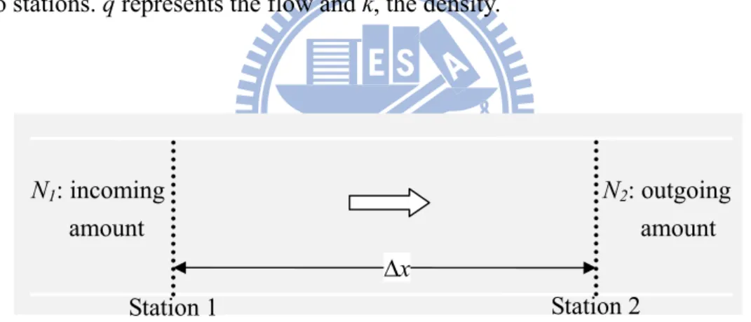
density, and speed. For a road section with an upstream and downstream observing station (as shown in Figure 2-1), the conservation law can be simply formulated as the equations (2-1~2-3) (Kühne, 1998): t N N q 2 1 (2-1) x N N k ( 2 1) (2-2) 0 t k x q (2-3)
where N1 represents the incoming vehicles amount passing station 1 for a period of
time, ∆t. N2 is the outgoing vehicles amount passing station 2. ∆x is the distance between
these two stations. q represents the flow and k, the density.
FIGURE 2-1 An illustration for the road section with two observing stations.
For a freeway with entering or exiting traffic, the continuity of the traffic flow can be formulated as the equation (2-4). The k(x, t) represents the density and q(x, t) is the flow at location x at instant of time t. (Chowdhury et al., 2000):
in qout j j j q i i i x x t x x t x t x q t t x k 1 1 ) , ( ) , ( ) , ( ) , ( (2-4) Station 1 Station 2 N1: incoming amount ∆x N2: outgoing amountwhere the first term on the right hand side,
in q i i i x x t 1 ) , ( represents entering sources at the qin on-ramps located at xi (i=1,2,…,qin). The next term on the right hand side,
out q j j j x x t 1 ) , ( takes care of exiting sinks, the qout off-ramps located at xj (j=1,2,…,qout).
The above equation (2-4) can be further simplified, if it reflects a highway with no entries or exits ramp. Under such special circumstances the equation (2-4) reduces to the simpler form (Lighthill and Whitham, 1955) as the following equation (2-5).
0 ) , ( ) , ( x t x q t t x (2-5)
2.1.2 LWR model ( Lighthill-Whitham-Richards model)
Lighthill and Whitham (1955) and Richards (1956) used the hypothesis about the fundamental diagram. The flow rate q is a function of the vehicle density ρ:
) ( q
q (2-6)
Using equation (2-6), the balance equation (2-5) takes the form as equation (2-7):
0 )) , ( ( ) , ( x t x q t t x (2-7)
Therefore, there is now only one independent variable in the equation (2-7), the vehicles density ρ (Figure 2-2). This makes it possible to solve this equation if initial and boundary conditions are given. Thus, the application of the hypothesis about the fundamental diagram leads to a solvable traffic flow model.
fl
ow
r
ate
density
slope v
FIGURE 2-2 The theoretical fundamental diagram.
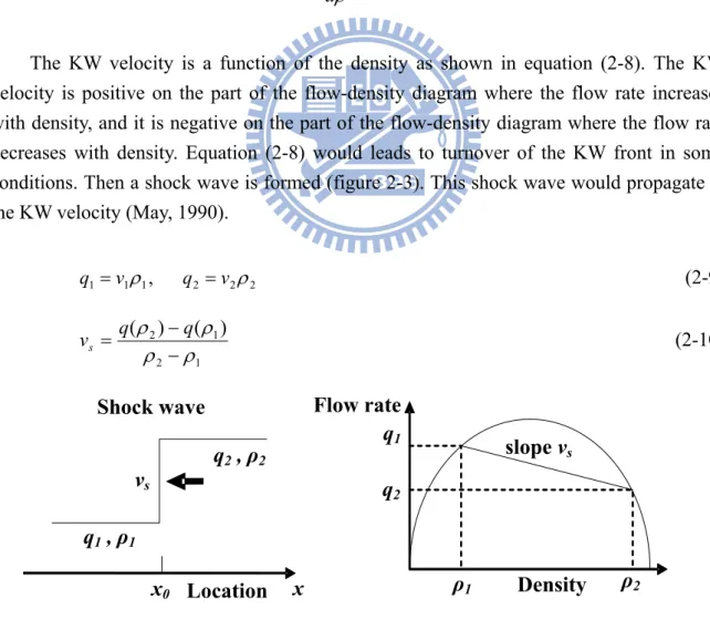
Solutions of the Lighthill-Whitham-Richards (LWR) model, equation (2-6), (2-7) are kinematic waves moving with the velocity.
Kinematic Waves (KW) d dq c ( ) (2-8)
The KW velocity is a function of the density as shown in equation (2-8). The KW velocity is positive on the part of the flow-density diagram where the flow rate increases with density, and it is negative on the part of the flow-density diagram where the flow rate decreases with density. Equation (2-8) would leads to turnover of the KW front in some conditions. Then a shock wave is formed (figure 2-3). This shock wave would propagate at the KW velocity (May, 1990).
2 2 2 1 1 1 v , q v q (2-9) 1 2 1 2) ( ) ( q q vs (2-10)
FIGURE 2-3 Representation of a shock wave in space and in the fundamental diagram. Flow rate Density slope vs q1 x q2 , ρ2 Shock wave vs q 2 ρ1 ρ2 x0 q1 , ρ1 Location
2.2 Microscopic approaches
The microscopic models, on the other hand, describe the interrelationship of individual vehicle movements interacted with other vehicles. These models of vehicular traffic attention are focused on individual vehicle each of which is represented by a “particle”. Car-following models are the most pertinent ones to explicate the one-dimensional movements in a longitudinal lane such that the following vehicle adjusts its speed to maintain desirable or safe distance headways with the lead vehicle. Stimulus-response model is perhaps the most prominent type developed in the 1950s and 1960s by the General Motors (GM) research group, which is still being applied or extended (Rothery, 1998; Brackstone, and McDonald, 1999; Chakroborty, and Kikuchi, 1999; Lan, and Yeh, 2001). The main concepts are described as follows:
2.2.1 Stimulus-Response model
The concept of car following on a motorway indicates a driver reacts to the altering headway with his predecessor the behavior of a driver. The main idea is that a driver will through control of the vehicle deceleration and acceleration to maintain a suitable distance and time gap between it and the vehicle that precedes it in the same lane. Many studies have been devoted to find mathematical formulas to descript the following behavior of the individual driver. The starting point of define the equation of motion is usually the analogue of the Newton’s equation for each individual vehicle. In Newtonian mechanics, the acceleration of the vehicle may be considered as the vehicle response to stimulus from other vehicle. This approach assumes within a range of distance, a stimulus-response relationship exist. The basic stimulus-response equation can be expressed as follows:
n n stimulus response] [ ]
[ (2-11)
where n represents number of vehicle. λ is a proportionality factor.
The stimulus function can be composed of many factors: the speed of the vehicle, distance headway (spacing), relative speed, etc. Each driver can respond to the surrounding traffic conditions only by accelerating or decelerating the vehicle. Different forms of the equations of motion of the vehicles in the different versions of the car-following models arise from the differences in their postulates regarding the nature of the stimulus. The
where xn(t) is the location of the nth vehicle at time t. The stimulus-response
relationship can be further expressed as follow equation (2-13): ) , , ( n n n sti n f v x v x (2-13)
where the function f represents the stimulus by the nsti th vehicle. v is the speed, n ∆xn represents the distance headway (spacing), ∆vn represents relative speed of the nth
vehicle, accordingly.
2.2.2 Follow-the-leader model
Chandler et al. (1958) proposed the first follow-the-leader model, the different in the velocities of the following nth and the leading n+1th vehicles was supposed to be the stimulus for the nth vehicle as shown in equation (2-14). It was assumed that every driver be likely to keep with the synchronized velocity as that of the front vehicle. Joining the equation (2-12) into equation (2-14), the stimulus-response relationship becomes equation (2-15): ) ( ) ( ) ( ] [stimulus n tT vn1 t vn t (2-14) )] ( ) ( [ ) (t T x 1 t x t xn n n (2-15)
where T is a response time.
2.2.3 Pipes car-following model
Pipes (1953) car-following theory is a linear model that depicts vehicular traffic behavior. The equation is derived by differentiating from equation (2-15) with respect to time. The first term of equation (2-16) in right hand side means that with the purpose of avoid crash with the leading vehicle, each driver must keep a safe distance ((∆x)safe) from
the leading vehicle. The second term of equation (2-16) in right hand side represents that: if the velocity of the nth vehicle is higher, the spacing to its leading vehicle needs to keep larger. It can be further explain that drivers obey the driving laws recommended in the California Motor Vehicle Code, leave one car length in front for every 10 miles per hour of speed increase. The equation can be expressed as the form:
) ( ) ( ) ( ) ( ) (t x 1 t x t x x t xn n n safe n (2-16)
where τ sets the time scale.
Forbes et al. (1958, 1963) proposed that the reaction time, τ, is larger when the distance headway increases and vice versa. The main concepts of Forbes’s car-following model can be expressed as equation (2-17).
)) ( ) ( ( 1 ) (t x 1 t x t xn n n (2-17) 2.2.4 GM Models
A series of models have been developed in the 1950s and 1960s by Herman and his colleagues at the General Motors Research Laboratories (Chandler, Herman, and Montroll, 1958; Gazis, Herman, and Potts, 1959; Gazis, Herman, and Rothery, 1961) to address microscopic approaches that focused on describing the driver car-following behaviors. Five generations of the GM car-following models are recognized and they provided an essential contribution to realize the traffic flow. Nowadays they are still applied in various aspects, including traffic stability and safety studies, level of service and capacity analysis, driver’s reaction times, etc.
) 1 , 0 ( )] ( ) ( [ ) ( 1 1 t T x t x t m l xn n n (2-18)
where α is the sensitivity coefficient, a experimental constant independent of n, and α varies from 0.17~0.74. ) 1 , 0 ( )] ( ) ( [ ) ( 1 1 t T x t x t m l xn i n n (2-19)
where α1 is the coefficient for driving in platoon; α2 is the coefficient for driving not in
platoon. ) 1 , 0 ( )] ( ) ( [ ) ( ) ( ) ( 1 1 0 1 x t x t m l t x t x T t x n n n n n (2-20)
2.2.5 Car-following theory for multiphase
Zhang and Kim (2005) hypothesize that drivers drive differently in different traffic situations and present a new car-follow theory that can reproduce both the capacity drop and traffic hysteresis, two prominent features of multiphase vehicular traffic flow. Conventional car-following models treat both drivers and roads as homogeneous entities––that is, they are modeling identical drivers who travel on homogeneous roads (Figure 2-4 (a)). The traffic that produces capacity drops and hysteresis loops, on the other hand, comprises diverse groups of drivers who travel on inhomogeneous roads and may behave differently under different driving conditions. A plausible car-following theory that explains these nonlinear phenomena must consider these inhomogeneities (Figure 2-4 (b)).
(a) (b)
(Source: Zhang and Kim, 2005) FIGURE 2-4 Comparison the homogeneous and inhomogeneous car-following models
with fundamental diagrams.
2.2.6 Optimal velocity (OV) models
The main concept of the optimal velocity models is depicted the driving strategy of the driver when following the leading vehicle. The formulas can be expressed as equation (2-23): )] ( ) ( [ 1 ) (t V t v t x desired n n n (2-23)
where desired n
V is the desired speed of the nth vehicle at time t. In the equation (2-15) of follow-the-leader model, driver tends to keep the same speed of the leading vehicle,
) ( )
(t x 1 t
Vdesired n
n . The optimal velocity models assume that Vndesired depends on spacing, ∆xn of the nth vehicle as shown in equation (2-24). A more realistic model that driver can
keep optimal velocity based on corresponding spacing are shown in equation (2-25). (Bando et al., 1994; Bando et al., 1995; Nakanishi et al., 1997; Sugiyama and Yamada, 1997; Chowdhury et al., 2000) )] ( )) ( ( [ 1 ) (t V x t v t x opt n n n n (2-24) x x x x x x x v x f x V B B A A opt for for for 0 ) ( max (2-25)
The presentation of OV model depends intensively on the proper decision of the optimal velocity function. Through introduction of appropriate optimal velocity, some important macroscopic characteristics, such as traffic jam and hysteresis effects can be observed.
2.2.7 Traffic hysteresis models
Newell (1965) supposed that drivers react to a stimulus in a different way in their acceleration and deceleration behaviors (Figure 2-5(a)) and developed the hysteresis loop. Treiterer and Myers (1974) first propose the apparent experiment proof of the traffic hysteresis effect. In real traffic environment, the traffic metastable phases have been confirmed to exist, and to be the derivation of the traffic hysteresis. Since the traffic metastable phases, the relationship of traffic flow and density will not be one-to-one association. Koshi et al. (1983) analyzed empirical traffic data and proposed the well known flow–density diagrams (Figure 2-5(b)).
(a) (b)
(Source: Zhang and Kim, 2005) FIGURE 2-5 The relationship ofdrivers react to a stimulus.
2.2.8 Gap acceptance models
Gap acceptance models have shown success to capture drivers' decision to carry out various maneuvers (e.g. Mahmassani and Sheffi (1981), Hamed et al., (1997), Polus et al., (2003)). These models suppose the existence of a latent space, which is the value where drivers are unresponsive. More recently, Sheu (2008) proposed to introduce the theorem of quantum mechanics in optical flows to explain the motion-related perceptual phenomena and to model the induced car-following while vehicles approach the incident site in adjacent lanes.
2.3 Related CA approaches
Cellular automaton (CA) is a powerful tool to describe the phenomena of real traffic flows characterized with complex dynamic behaviors. Nagel and Schreckenberg (1992) first proposed the renowned NaSch model to reproduce the basic features of real traffic. In their model, the road is divided into squared-cells of length 7.5 meters. Each cell can either be empty or occupied by at most one car. The space, speed, acceleration and even the time are treated as discrete variables. The state of the road at any time-step is derived from one time-step ahead by applying acceleration, braking, randomization and driving rules for all cars at the same time (i.e., parallel dynamics). Obviously, their coarse description of cells is an extreme simplification of the real world conditions. Therefore, a considerable number of modified NaSch CA rules have been found in the past decade (for instance, Nagel et al. (1996, 1998); Rickert et al. (1996); Chowdhury et al. (1997); Barlović et al. (1998)). Other related works that improved NaSch coarse cells with finer cells have also been found (for
instance, Knospe et al. (2000); Bham and Benekohal (2004); Lan and Chang (2003, 2005); Lárraga et al. (2005)). In addition, Wolf (1999) employed a modified NaSch model to address the metastable states at the jamming transition in detail. Wang et al. (2000) introduced NaSch model and Fukui-Ishibashi model to investigate the asymptotic self-organization phenomena of one-dimensional traffic flow. Pottmeier et al. (2002) studied the impact of localized defect in a CA model for traffic flow exhibiting metastable states and phase separation.
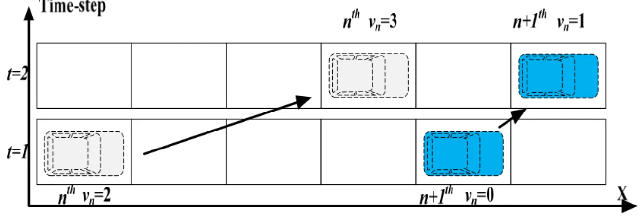
2.3.1 NaSch model
NaSch model was proposed by K. Nagel & M. Schreckenber in 1992. Capable of reproduce important entities of real traffic flow, e.g. density-flow relation. Model description, one-lane traffic, divided into cells of length 7.5 m. Each cell can either be empty or occupied by at most one car with discrete velocity: v={0, …, vmax} (Figure 2-6).
The state of road at time t+1 can be obtained from that at time t by applying the following forward rules:
Step 1 : Acceleration vn = min (vn + 1, vmax) (2-26)
Step 2 : Braking vn = min (vn, dn - 1) (2-27)
where dn is the distance-headway to next vehicle ahead.
Step 3 : Randomization with probability p
vn = max (vn - 1, 0) (2-28)
Step 4 : Driving xn = xn + vn (2-29)
where xn is the position of nth vehicle.
The NaSch model is a minimal model in the sense that all the four steps are necessary to reproduce the basic features of real traffic; however, additional rules need to be formulated to capture more complex situations.
FIGURE 2-6 The action of a single-lane NaSch cellular automaton model.
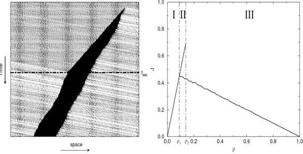
2.3.2 Velocity-Dependent Randomization (VDR) Model
Barlovic, et. al. (1998) based on the original NaSch model, for sake of simulating the phase separation phenomena in real world (Figure 2-7). The randomization parameter is set as: states metastable in flow i.e. , 0 jam from outflow i.e. , 0 ) ( 0 v for P v for P v P n n n (2-30)
Usually P0 < Pn , as to reflect the fact that when driving out from the downstream of
jams, drivers are more likely to postpone acceleration. This is the so-called slow-to-start case. The state of road at time t+1 can be obtained from that at time t by applying the following rules:
Step 0 : randomization parameter Pn = P(vn) (2-31)
Step 1 : Acceleration vn = min (vn+1, vmax) (2-32)
Step 2 : Braking vn = min (vn , dn -1) (2-33)
Step 3 : Radomization with probability pn n n n n n P v P v v 1 y probabilit h wit y probabilit ith w ) 0 , 1 max( (2-34) Step 4 : Movement xn = xn+ vn (2-35)
(Source: Barlović, 2003) FIGURE 2-7 Space-time diagram and fundamental diagram of a spontaneously
emerging jam.
2.3.3 Comfortable Driving (CD) Model
Knospe, et al. (2000) based on original VDR model and the following driving strategy. At large distances the cars move (apart from fluctuations) with their desired velocity vmax. At
intermediate distances drivers react to velocity changes of the next vehicle downstream, i.e. to ‘brake lights’. At small distances the drivers adjust their velocity such that safe driving is possible. The acceleration is delayed for standing vehicles and directly after braking events.
Randomization parameter P is decided through equation (2-36): cases other all in 0 if and 1 if )) ( ), ( ( 0 1 1 d n s h n b n n n P v P t t b p t b t v P (2-36)
where P0, Pd and Pb, depends on the current velocity vn and bn is the status of the brake
light (on (off)→bn = 1 (0)). bn1(t) is the status of the brake light of preceding vehicle
Step 0 : Randomization parameter Pn P(vn(t),bn1) (2-37) Step 1 : Acceleration if (bn10&bn 0) or th ts
then vn(t1)min(vn(t)1,vmax) (2-38) Step 2 : Braking ( 1) ( ( ), eff)
n n
n t v t d
v
if vn(t1)vn(t)then bn 1 (2-39) where n max( anti gap ,0)
eff
n d v
d ; vanti min(vn1 ,dn1)
Step 3 : Randomization if (rand()<P) then vn(t1)max(vn(t1)1 ,0)
if P = Pb ,then bn=1. (2-40)
Step 4 : Movement xn(t1)xn(t)vn(t1) (2-41)
(Source: Knospe, et al., 2000) FIGURE 2-8 Comparison the CD model simulation result (left) with empirical data
(right).
The simulation results of the approach show that the empirical data are reproduced in great detail (Figure 2-8).
2.3.4 Three-Phase traffic Theory
Boris Kerner (2004), a German traffic physician, introduced a three-phase traffic theory which consists of free flow, synchronized flow and wide moving jam phases. The later two phases exist in congested states where downstream front of the synchronized flow phase is often fixed at a bottleneck but the wide moving jam will propagate through the spatial locations of the bottleneck.
To explore the emergence of such traffic patterns, Kerner and partners have shown complex spatiotemporal behaviors based on empirical freeway traffic analysis (Figure 2-9) (see, for example, Kerner and Rehborn (1996); Kerner (1998); Kerner and Klenov (2002); Kerner et al. (2002); Kerner and Klenov (2004)). The effect of slow cars in two-lane systems was further studied by Knospe et al. (1999) who found that even few slow cars could initiate the formation of platoons at low densities.
Moreover, Kerner (2005) also compared the congested pattern control approach with the free flow control approach at an on-ramp bottleneck with ramp metering. It was found that the congested pattern control approach has higher throughputs on the main road downstream of the bottleneck and considerably lower vehicle waiting times at the light signal on the on-ramp. The upstream propagation of congestion does not occur even if large amplitude perturbations appear in traffic flow.
2.4 Summary
Most of the aforementioned conventional traffic flow models are based on the assumption of the homogeneity of the system. In addition, recent CA models are mainly developed assuming identical vehicle parameters. These models can be used to simulate the interactions of individual vehicles in traffic vehicular system; however, they cannot demonstrate the real vehicle traffic conditions due to the lack of consideration of the driver heterogeneity in individual characteristics and driving behaviors. In reality, mixed traffic is prevailing around the world either in developed or under developing countries. Some of such different-dimensioned vehicles, with different in length and width, may share the same lane while moving. Moreover, these vehicles also move with different parameters (e.g., different acceleration/deceleration rate, different desired speeds and safe driver speeds). There are heterogeneous driving behaviors across drivers with very different characteristics. It is always important to capture the traffic flow features so that more realistic traffic flow models can be developed to better represent the prevailing traffic situations.
Chapter 3 DEFINITIONS
This chapter introduces the definitions applied in this research. Section 3.1 addresses the common unit for cells and sites; the global traffic variables are introduced in Section 3.2; the local traffic variables are introduced in Section 3.3, followed by a summary in Section 3.4.
3.1 Common Unit for Cells and Sites
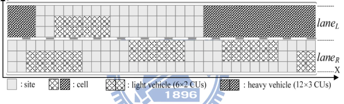
Lan and Chang (2005) first developed inhomogeneous CA models to elucidate the interacting movements of cars and motorcycles in mixed traffic on surface roads. The car and motorcycle in their study are represented by non-identical particle sizes that occupy 6×2 and 2×1 cell units, respectively. Each cell is a squared grid of 1.25×1.25 meters, which is regarded as a “common unit (CU)” of the non-identical vehicle sizes. The concept of CU has advantages of describing the inhomogeneous vehicle sizes and of accommodating non-identical lane widths in various roadway environments, while CA simulations are performed. This research continues to use the word “cells” to describe the vehicles but will use the concept of CU to gauge the different vehicle types. In line with the physical dimensions and their required clearances for safe movement, for instance, a bicycle or a motorcycle can be defined as a small-sized particle of 2×1 CUs. A car can be defined as a median-sized particle of 6×2 CUs. A single-unit truck or a regular bus can be defined as a large-sized particle of 12×3 CUs. Of course, other types of vehicles, such as rickshaw or tricycle, semi-trailer, trailer, twin-truck, and articulated bus, can also be defined in terms of different common units of cells.
To accommodate different vehicle types moving in various widths of lanes or roadways, this research uses another term, “sites,” to represent the two-dimensional roadway space. This research propose the CA traffic simulation models to elucidate the behavior of vehicles moving in a longitudinal (X) direction and transverse (Y) direction of a two-dimensional (2-D) roadway space. The dimensions of sites, cells and the rules of vehicle movements are defined in such a way that they can best conform to the mixed traffic context. The roadway is composed of numerous identical “sites,” each of which is also a squared grid of 1.25×1.25 meters, which has exactly the same size as one cell, the basic CU in gauging the vehicles. Thus, each “site” in this study will be exactly occupied or
To further reflect the situations for Taiwan freeways where speed limit is 110 kph, this study continues to use the concept of CU proposed by Lan and Hsu (2005, 2006), but will reduce the CU size to a grid of 1.25×1.0 meters. Therefore, the maximum speed of CA simulations can be set equal to 31sites/sec (111.6 kph), very close to the speed limit (110 kph), and the incremental speed for vehicles is 1 meter per time-step (3.6 kph). Since each “site” will also be exactly occupied or unoccupied by a “cell,” the dimension of a “site” in this study must be defined as a grid of 1.25×1.0 meters. A 3.75-meter (12-feet) standard freeway lane is equivalent to a lane width of “three sites.” Likewise, a 2.5-meter urban narrow street can be regarded as a lane width of only “two sites.” Accordingly, a car is defined as a median-sized particle of 2×6 cells whereas a twin-truck is defined as a super large-sized particle of 3×24 cells. Of course, other types of vehicles, such as motorcycle, bus, and single-unit truck can also be defined in terms of different common units of cells.
FIGURE 3-1 Heterogeneous vehicle sizes and roadway spaces defined by a common unit (CU) of grid-cell and grid-site.
3.2 Global Traffic Variables
3.2.1 Generalized Traffic Variables 1. Density
The conventional density at a specific time t over a road section of length L is defined as the number of vehicles n(t) observed in a photograph of the section at the given time divided by the length of the section, expressed in first term of eq. (3-1). Multiplying the numerator and denominator of this expression by a small time interval, ∆t, the average density over a thin vertical rectangular region L×∆t formed by the dotted lines of Figure 3-2 can be defined as “the ratio of total time spent in time-space region (e.g., veh-hrs.) to the area of that time-space region (e.g., mile-hrs.),” also expressed in eq. (3-1), see, for example, Daganzo (1997).
t L t t n L t n t k ( ) ( ) ) ( (3-1)
The density over a large rectangular region A, of length L and width T formed by the bold lines of Figure 3-2, k(A), can therefore be defined as:
A A t t L t t n A k t t ( ) ) ( ) (
(3-2)where t(A) is the total time spent in A and |A| denotes the area of A.
FIGURE 3-2 An illustration of generalized definition of density over a space-time rectangular region.
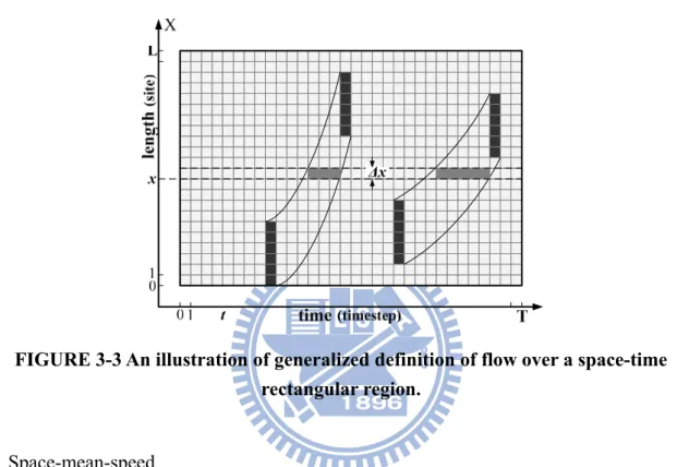
2. Flow
The conventional flow rate at a specific stationary location x over a period of observed time T is defined as the number of vehicles m(x) passing through that stationary location divided by the period of time, expressed in first term of eq. (3-3). Likewise, multiplying the numerator and denominator of this expression by a small distance interval, ∆x , the average flow over the thin horizontal rectangular region T×∆x formed by the dotted lines of Figure 3-3 can be defined as “the ratio of total distance traveled in time-space region (e.g.,
Thus, the flow over the same rectangular region A, of length L and width T formed by the bold lines of Figure 3-3, q(A) , can be defined as:
A A d x T x x m A q x x ( ) ) ( ) (
(3-4)where d(A) represents the total distance traveled in A.
FIGURE 3-3 An illustration of generalized definition of flow over a space-time rectangular region.
3. Space-mean-speed
The ratio of eq. (3-4) to eq. (3-2) becomes the space-mean-speed in A, which can be further reduced to “the ratio of the total distance traveled to the total time spent by all vehicles in A,” as expressed in eq. (3-5):
) ( ) ( ) ( ) ( ) ( A t A d A k A q A v (3-5)
3.2.2 Spatiotemporal Traffic Variables
The above generalized density, flow and speed are defined on vehicle (or particle) basis over a 2-D time-space region (Daganzo, 1997). Such definitions may not exactly depict the collective behaviors of traffic moving over a 3-D domain, including 2-D for the roadway (longitudinal and transverse) and 1-D for the time. To be precise in the CA simulations, this research need to redefine the traffic variables in a 3-D spatiotemporal domain on site or cell basis, not on vehicle basis. Therefore, the study proposes new
definitions of traffic variables in spatiotemporal sense so as to precisely facilitate the following simulations on various sizes of vehicles sharing the same “lane” in mixed traffic contexts.
To regard a vehicle as several cells and to reflect the realistic traffic movement in a 2-D road, this study defines the instantaneous approach-based occupancy (ρ(t)) , a proxy of instantaneous density, as:
N t N N t N t y y o
) ( ) ( ) ( 0 (3-6)where the denominator N stands for the total number of sites in road and the numerator N0(t) represents the total number of sites occupied by cells of vehicles at instantaneous time
t in road. Hence, N-N0(t) represents the instantaneous total number of empty (unoccupied)
sites in road. N0∆y(t) represents the total number of sites occupied by cells in the specific
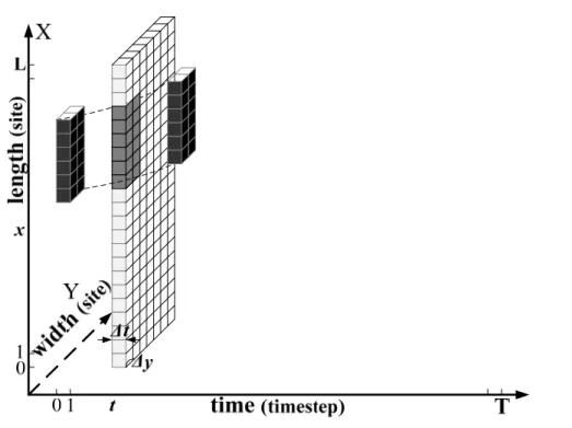
transverse slice ∆y at instantaneous time t . Figure 3-4 and figure 3-5 illustrate the instantaneous approach-based occupancy that is summation all the specific transverse slice ∆y at instantaneous time t.
FIGURE 3-5 Vehicular trajectories over a specific transverse slice in a spatiotemporal domain enclosed by L×W×∆t.
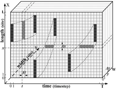
Figure 3-6 illustrates the trajectories of three light vehicles (each represented by 6×2 CUs) in a specific transverse slice (e.g.,y1) of a spatiotemporal domain S enclosed byLW T, where L denotes the longitudinal length (x1 ,2 ,3 ,...,L), W the transverse width (y1 ,2 ,3 ,...,W ) of a roadway, and T the number of observed time-steps (t1 ,2 ,3 ,...,T ). In this spatiotemporal domain S enclosed by L×W×T, if one repeats the same procedure from eq. (3-1) to eq. (3-2), a similar but more generalized definition of occupancy over this spatiotemporal domain S, ρ(S) , can be defined as eq. (3-7):
S S t t N t t N S t t ( ) ) ( ) ( 0
(3-7)where t(S) is the total time spent by all cells in S; t(S) = ∑ N0(t)∆t. |S| represents the
‘volume’ of this spatiotemporal domain S. Likewise, a more generalized definition of flow in the spatiotemporal domain S can be defined as eq. (3-8):
S S d x T x x M S q x x ( ) ) ( ) ( 0
(3-8)where M0(x) is the total number of sites occupied by cells of vehicles at a specific
location x in road. d(S) is the total distance traveled by all cells of vehicles in the space S; d(S) = ∑ M0(x)∆x.
FIGURE 3-6 Vehicular trajectories over a specific transverse slice in a spatiotemporal domain S enclosed by L×W×T.
The ratio of eq. (3-8) to eq. (3-7) defines the generalized space-mean-speed in S, which can be further reduced to the ratio of the total distance traveled to the total time spent by all cells in S, as expressed in eq. (3-9):
) ( ) ( ) ( ) ( ) ( S t S d S S q S v (3-9)
The above generalized definitions of average spatiotemporal occupancy, flow and speed of “cells” moving over 3-D (2-D sites plus 1-D time-step) spatiotemporal domain, as expressed in eqs. (3-7), (3-8) and (3-9), are used in the following CA simulations to describe the collective behaviors of traffic flow patterns.
3.3 Local Traffic Variables
The localized definitions of occupancy, flow and speed of “cells” moving over a virtual detector, as expressed in equations. (3-10), (3-11) and (3-12), are used in the following CA simulations:
2. Occupancy
Occupancy (proxy of density), ρ(L), is the portion of this time-step that “cells” are over the virtual detector on road.
n v W N L ) ( (3-11) 3. Speed
Speed, v(L), is average the actual speed of the n-th vehicle.
vn N L v( ) 1 (3-12) 3.4 Simulation settingThe simulations in the following chapters are performed on a closed track containing 6×1,800 site CUs, which represents a two-lane freeway mainline of width 7.5 meters and length 2,250 meters (length of site 1.25 m) or 1,800 meters (length of site 1 m). We simulate various occupancy scenarios for 600 time-steps. Initially, all the vehicles are set equally spaced or line up from end of road section on the circular track, with speed 0 at time-step 0. To avoid the initial settings biasing the simulated results, the first 30 time-steps are viewed as the warm-up period. Thus, the average occupancy, flow and speed over a spatiotemporal domain are calculated from the 31st time-step to the end at the 630th
time-step (Figure 3-7).