以參考訊號架構為基礎之穩健語者定位與語音純化法

全文

(1)國立交通大學電機與控制工程學系博士論文. 以參考訊號架構為基礎之穩健語者定位與語音純化法 Robust Reference-signal-based Speaker’s Location Detection and Speech Purification. 研究生：鄭价呈指導教授：胡竹生教授. 中華民國九十五年六月 i.

(2) 以參考訊號架構為基礎之穩健語者定位與語音純化法 Robust Reference-signal-based Speaker’s Location Detection and Speech Purification 研究生：鄭价呈. Student：Chieh-Cheng Cheng. 指導教授：胡竹生. Advisor：Jwu-Sheng Hu 國立交通大學. 電機與控制工程學系博士論文. A Dissertation Submitted to Department of Electrical and Control Engineering College of Electrical Engineering and Computer Science National Chiao Tung University in partial Fulfillment of the Requirements for the Degree of Doctor of Philosophy in Electrical and Control Engineering June 2006 Hsinchu, Taiwan, Republic of China. 中華民國九十五年六月 ii.

(3) 國. 立. 交. 通. 大. 學. 博碩士論文全文電子檔著作權授權書 (提供授權人裝訂於紙本論文書名頁之次頁用). 本授權書所授權之學位論文，為本人於國立交通大學電機與控制工程所. 94. 學年度第二_學期取得博士學位之論文。. 論文題目：以參考訊號架構為基礎之穩健語者定位與語音純化法指導教授：胡竹生. ■ 同意 □不同意本人茲將本著作，以非專屬、無償授權國立交通大學與台灣聯合大學系統圖書館：基於推動讀者間「資源共享、互惠合作」之理念，與回饋社會與學術研究之目的，國立交通大學及台灣聯合大學系統圖書館得不限地域、時間與次數，以紙本、光碟或數位化等各種方法收錄、重製與利用；於著作權法合理使用範圍內，讀者得進行線上檢索、閱覽、下載或列印。論文全文上載網路公開之範圍及時間：本校及台灣聯合大學系統區域網路校外網際網路. ■ 中華民國 95 年 9 月 30 日公開 ■ 中華民國 95 年 9 月 30 日公開. 授權人：鄭价呈. 親筆簽名：中華民國. 95. 年. 8. 月 iii. 22. 日.

(4) 國. 立. 交. 通. 大. 學. 博碩士紙本論文著作權授權書 (提供授權人裝訂於全文電子檔授權書之次頁用). 本授權書所授權之學位論文，為本人於國立交通大學電機與控制工程所 94 學年度第二_學期取得博士學位之論文論文題目：以參考訊號架構為基礎之穩健語者定位與語音純化法指導教授：胡竹生 ■ 同意本人茲將本著作，以非專屬、無償授權國立交通大學，基於推動讀者間「資源共享、互惠合作」之理念，與回饋社會與學術研究之目的，國立交通大學圖書館得以紙本收錄、重製與利用；於著作權法合理使用範圍內，讀者得進行閱覽或列印。本論文為本人向經濟部智慧局申請專利(未申請者本條款請不予理會)的附件之一，申請文號為：____________________，請將論文延至____年____月____日再公開。. 授權人：鄭价呈. 親筆簽名：中華民國. 95. 年. 8. 月. iv. 22. 日.

(5) 以參考訊號架構為基礎之穩健語者定位與語音純化法研究生：鄭价呈. 指導教授：胡竹生博士. 國立交通大學電機與控制工程學系(研究所)博士班. 摘要使用麥克風陣列來改善語音擷取的品質以及偵測語者方位在語音介面相關研究上非常重要。本研究的目的在於利用ㄧ組線性麥克風陣列以及參考訊號來定位某些特定所需之語者，並且提升語音辨識的正確性。本篇論文中所提出之方法皆是利用參考訊號為基礎的系統架構來間接地解決麥克風間匹配性問題。本篇論文所提出的語者定位法則利用高斯混合模型來針對每個位置所獨具的特徵(相位差分布)作出模型化的動作。此語者定位方法可以抵抗背景雜音與反射效應，並於近場與遮蔽的環境中提供準確的語者定位結果。為了減低運算複雜度，本篇論文提出了兩種頻域語音純化法(SPFDBB 與 FDABB)。有ㄧ法則為：若在時域中語音訊號與通道之間的關係為捲積，則對應於頻域中這兩者的關係則變為一般的乘積。但是此法則並不適用於時域的濾波器階數大於轉換到頻域所取用的窗長度之情況中。因此，本論文所提出的語音純化法便將多個窗的資料結合在一起共同處理，以期能盡可能的逼近以上之法則。此外，還提出了一個參數以提供使用者可針對通道補償以及雜訊抑制來訂定不同的權重。提供上述功能的語音純化法稱之為 SPFDBB。但若同時將太多個窗之資料統一處理，則此語音純化法便不適用於一會經常性變動的環境中。因而本論文又更進ㄧ步地提出新參數稱為 CBVI 來自動調整窗之個數。結合此 CBVI 參數與 SPFDBB 之語音純化法則稱之為 FDABB。除了上述幾個議題外，模型化誤差亦為ㄧ重要課題。對此，本論文針對一著名理論稱之為 H∞ 理論做出相關研究，進而將其套用於所提出之兩種語音純化法中。最終，本論文利用模擬以及實際環境下的實驗結果來說明所提出方法的可行性。. v.

(6) Robust Reference-signal-based Speaker’s Location Detection and Speech Purification Graduate Student: Chieh-Cheng Cheng. Advisor: Dr. Jwu-Sheng Hu. Department of Electrical and Control Engineering National Chiao-Tung University. Abstract The use of microphone array to enhance speech reception and speaker localization is very important. The objective of this work is to locate speakers of interest and then provide satisfactory speech recognition rates using a linear microphone array. The proposed approaches utilize a reference-signal-based architecture to indirectly solve a practical issue, microphone mismatch problem. Additionally, the proposed speaker’s location detection method utilizes Gaussian mixture model (GMM) to model a corresponding phase difference distribution for each specific location of the speaker. The proposed localization approach is useful in the presence of background noise and reverberations. Even under near-filed and non-line-of-sight environments, the approach can still provide high detection accuracy. In. terms. of. effectiveness,. the. proposed. beamformers,. soft. penalty. frequency-domain block beamformer (SPFDBB) and frequency-domain adjustable block beamformer (FDABB) are designed in the frequency domain. However, due to the fact that the convolution relation between channel and speech source in time-domain cannot be modeled accurately as a multiplication in the frequency domain with a finite window size, the proposed beamformers put several frames into a block to approximate the transformation. Furthermore, to put different emphases on vi.

(7) channel recovery and noise suppression, a parameter named soft penalty is designed. Note that for a highly variant environment, it is not suitable to allocate too many frames into one block. Therefore, the SFPDBB is extended to the FDABB with a measurement index, named CBVI, which enables the FDABB to automatically adjust the number of frames. An H∞ adaptation criterion is also investigated and applied to enhance the robustness to the modeling error. Finally, the results from simulations and practical experiments are provided as proof of the effectiveness and usefulness of these proposed approaches.. vii.

(8) Contents Chapter 1 Introduction ................................................................................................1 1.1 1.2. Overview of Direction of Arrival Algorithms............................................3 Overview of Beamformers.........................................................................6 1.2.1 Fix-coefficients beamformers ........................................................7 1.2.2 Post-filtering beamformers ............................................................8 1.2.3 Subspace beamformers ..................................................................8 1.2.4 Adaptive beamformers...................................................................9 1.3 Outline of Proposed System.......................................................................9 1.3.1 VAD Algorithm..............................................................................9 1.3.2 Reference-signal-based Speaker’s Location Detection Algorithm 11 1.3.3 Reference-signal-based Frequency-Domain Beamformer...........12 1.4 Contribution of this Dissertation..............................................................14 1.5 Dissertation Organization ........................................................................15 Chapter 2 Reference-signal-based Time-domain Adaptive Beamformer .................16 2.1 Introduction..............................................................................................16 2.2 System Architecture .................................................................................18 2.3 Summary ..................................................................................................23 Chapter 3 Reference-signal-based Frequency-domain Adaptive Beamformer ........24 3.1 Introduction..............................................................................................24 3.2 System Architecture .................................................................................26 3.3 SPFDBB Using NLMS Adaptation Criterion ..........................................27 3.4 FDABB and Computational Effort Analysis ...........................................32 3.4.1 FDABB Using NLMS Adaptation Criterion................................32 3.4.2 Computational Effort Analysis ....................................................34 3.5 Frequency-domain Performance Indexes ................................................35 3.6 Summary ..................................................................................................37 Chapter 4 H∞ Adaptation Criterion ...........................................................................38 4.1. Introduction..............................................................................................38 4.2.. Time-Domain Adaptive Beamformer Using H∞ Adaptation Criterion ....39 4.2.1. Definition of H∞ -norm.................................................................40 viii.

(9) 4.2.2. Formulation of Time-Domain Adaptive Beamformer .................40. 4.2.3 Solution of suboptimal H∞ Adaptation Criterion.......................43 4.2.4 Solution of Time-domain Adaptive Beamformer ........................44 4.3. SPFDBB, FDABB and Computational Effort Analysis ..........................46 4.3.1 SPFDBB Using H∞ Adaptation Criterion..................................46 4.3.2 FDABB Using H∞ Adaptation Criterion ...................................49 4.3.3 Computational Effort Analysis ....................................................50 4.4. Time-domain Performance Indexes .........................................................51 4.5. Summary ..................................................................................................52 Chapter 5 Reference-signal-based Speaker’s Location Detection............................54 5.1 Introduction..............................................................................................54 5.2 System Architecture .................................................................................58 5.2.1 System Architecture .....................................................................58 5.2.2 Frequency Band Divisions based on a Uniform Linear Microphone Array........................................................................................59 5.3 Location Model Description and Parameters Estimation ........................60 5.3.1 GM Location Model Description.................................................61 5.3.2 Parameters Estimation via EM Algorithm ...................................63 5.4 Single Speaker’s Location Detection Criterion .......................................65 5.5 Testing Sequence Lengths and Thresholds Estimation............................66 5.6 Multiple Speakers’ Locations Detection Criterion...................................70 5.7 Summary ..................................................................................................71 Chapter 6 Experimental Results................................................................................73 6.1 Adaptive Beamformers Using NLMS Adaptation Criterion ...................74 6.1.1 Simulation Results .......................................................................74 6.1.2 Indoor Environment .....................................................................81 6.1.3 Vehicular Environment ................................................................84 Comparison of NLMS and H∞ Adaptation Criterions .............................85 6.2.1 Simulation Results .......................................................................85 6.2.2 Indoor environment......................................................................90 6.2.3 Vehicular Environment ................................................................91 6.3 Reference-signal-based Speaker’s Location Detection............................92 6.3.1. Vehicular Environment ................................................................92 6.3.2. Indoor Environment ...................................................................101 6.4 Summary ................................................................................................106. 6.2. ix.

(10) Chapter 7 Conclusions and Future researches ........................................................108 7.1. Conclusions............................................................................................108 7.2. Future researches ...................................................................................109 Reference ...................................................................................................................113. x.

(11) Index Automatic speech recognition (ASR) ..........................................................................16 Constant directivity beamformer (CDB) .......................................................................7 Delay-and-sum (DS) ....................................................................................................16 Discrete Fourier transform (DFT)................................................................................24 Direction of Arrival (DOA) ...........................................................................................3 Finite impulse response (FIR)........................................................................................7 Frequency-domain adjustable block beamformer (FDABB).......................................12 Generalized singular value decomposition (GSVD)......................................................8 Generalized sidelobe cancellation (GSC) ....................................................................16 Human-computer interaction (HCI)...............................................................................1 Linearly constrained minimum variance (LCMV) ......................................................16 Normalized least mean square (NLMS) ........................................................................8 Noise suppression ratio (NSR).....................................................................................26 Short time Fourier transform (STFT) ..........................................................................25 Singular value decomposition (SVD) ............................................................................8 Soft penalty frequency-domain block beamformer (SPFDBB)...................................12 Source distortion ratio (SDR) ......................................................................................26 Time-difference of arrival (TDOA) ...............................................................................4 Voice activity detection (VAD) ......................................................................................9. xi.

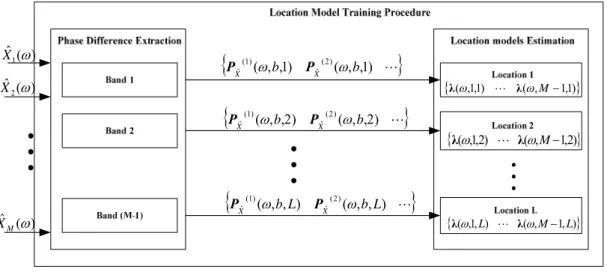
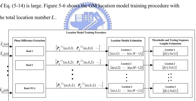
(12) List of Figures Figure 1-1 Block diagram of the general microphone-array-based speech enhancement system ......................................................................................................3 Figure 1-2 Microphone array configuration for plane or spherical wave hypothesis.3 Figure 1-3 Relation of eigenspaces.............................................................................5 Figure 1-4 Diagram of the beamformer ......................................................................6 Figure 1-5 Block diagram of proposed reference-signal-based speech enhancement system ............................................................................................................................9 Figure 1-6 Flowchart of the fundamental VAD algorithm........................................10 Figure 2-1 System architecture of the reference-signal-based time-domain adaptive beamformer ..................................................................................................................10 Figure 2-2 Installation of the array and headset microphone inside a vehicle..........19 Figure 2-3 Flowchart of the reference-signal-based time-domain adaptive beamformer ..................................................................................................................21 Figure 3-1 Overall system structure..........................................................................27 Figure 3-2 FDABB using NLMS adaptation criterion .............................................34 Figure 4-1 Transfer operator Z from input {ui } to output. {yi } ..............................40. Figure 4-2 System Architecture of the time-domain adaptive beamformer using H∞ adaptation criterion…………………………………………………………………...41 Figure 4-3 Transfer operator from disturbances to coefficient vector estimation error ......................................................................................................................................42 Figure 4-4 System Architecture of SPFDBB and FDABB using H∞ adaptation criterion ........................................................................................................................42 Figure 4-5 FDABB using H∞ adaptation criterion....................................................50 Figure 5-1 Proposed reference-signal-based speaker’s location detection system architecture...................................................................................................................59 Figure 5-2 Microphone array geometry....................................................................60 Figure 5-3 Location model training procedure with the total location number L ..65 Figure 5-4 The histograms of phase differences at locations No. 1, 2, and 1 and 2 between the third and the sixth microphones at a frequency of 0.9375 kHz ...............65 Figure 5-5 A two people conversation condition......................................................65 Figure 5-6 Location model training procedure with testing sequence length and xii.

(13) thresholds estimation ...................................................................................................70 Figure 6-1 Processed frame window and overlapping condition..............................73 Figure 6-2 Arrangement of microphone array, noies and speech source in simulation experiments ..................................................................................................................75 Figure 6-3 NSR and SDR form C6 to C9 with channel response duration 1024. The dash-dot line represents C6 (L = 1), the dot line represents C7 (L = 10), the straight line represents C8 (L = 20), and the dash line represents C9 (L = 30) ........................77 Figure 6-4 CBVI in the first simulation experiment ...............................................78 Figure 6-5 NSR and SDR form C7 to C10 with channel response duration 1024. The dash-dot line represents C10 (L = 1), the dot line represents C7 (L = 10), the straight line represents C8 (L = 20), and the dash line represents C9 (L = 30) ........................78 Figure 6-6 CBVI in the second simulation experiment ..........................................79 Figure 6-7 NSR and SDR in the second simulation experiment. The dash-dot line represents C10 (L = 1), the dot line represents C7 ( L = 10 ), the straight line represents C8 ( L = 20 ), and the dash line represents C9 ( L = 30 )..............................................80 Figure 6-8 Arrangement of microphone array, noises and speech source in a noisy environment .................................................................................................................81 Figure 6-9 ASR rates of different kinds of beamformer outputs versus different experiment conditions..................................................................................................83 Figure 6-10 ASR rates of SPFDBB and FDABB versus different experiment conditions.....................................................................................................................83 Figure 6-11 ASR rates of reference-signal-based time-domain beamformer, SPFDBB and FDABB .................................................................................................85 Figure 6-12 Filtered output error ratios of NLMS adaptation criterion with the tap number of 10 and 20………………………………………………………………….87 Figure 6-13 Filtered output error ratios of H∞ adaptation criterion with the tap number of 10 and 20………………………………………………………………….87 Figure 6-14 Filtered output error versus seven conditions .......................................87 Figure 6-15 Coefficient vector estimation error versus seven conditions ................88 Figure 6-16 Reference signal estimation error versus seven conditions...................88 Figure 6-17 Filter coefficient estimation error ratios in three cases .........................89 Figure 6-18 ASR rates of SPFDBB and FDABB using NLMS and H∞ adaptation criterions in an indoor environment.............................................................................91 Figure 6-19 ASR rates of SPFDBB and FDABB using NLMS and H∞ adaptation criterions in a vehicular environment ..........................................................................92 Figure 6-20 Seat number and microphone array position.........................................93 Figure 6-21 Correct rate versus the different mixture numbers in 100 km/h............97 Figure 6-22 The histograms of phase differences at locations No. 2, 4, and 6 xiii.

(14) between the third and the sixth microphones at a frequency of 0.9375 kHz and between the fourth and the sixth microphones at a frequency of 1.5 kHz, e.g., in third and fourth frequency bands (speed = 100 km/h) .........................................................97 Figure 6-23 Locations number of the seats...............................................................99 Figure 6-24 Average correct rates versus the mixture numbers..............................100 Figure 6-25 Configuration of microphone array, noises and speech sources in noisy environment ...............................................................................................................102 Figure 6-26 Correct rates versus the different mixture numbers ............................104 Figure 6-27 Configuration of microphone array, noises and speech sources in noisy environment ...............................................................................................................105 Figure 6-28 Average correct rates versus the mixture numbers..............................105 Figure 7-1 Speech enhancement system with a combination of beamformer and recognizer................................................................................................................... 111 Figure 7-2 Overall system structure which integrates the speaker’s location detection approach and SPFDBB or FDABB............................................................112 Figure 7-3 Flowchart of the architecture which integrates the speaker’s location detection approach and SPFDBB or FDABB............................................................112. xiv.

(15) List of Tables Table 3-1 Table 4-1 Table 5-1 Table 6-1 Table 6-2 Table 6-3 Table 6-4 Table 6-5 Table 6-6 Table 6-7 Table 6-8 Table 6-9. Real Multiplication Requirement in One Second Input Data .................35 Real Multiplication Requirement in One Second Input Data .................51 Relationship of Frequency Bands to the Microphone Pairs ...................60 The First Simulation Experiment: Soft Penalty Parameter is 0 ..............76 The First Simulation Experiment: Soft Penalty Parameter is 2 ..............76 The First Simulation Experiment: Soft Penalty Parameter is 4 ..............76 Parameters of the FDABB ......................................................................77 Real Multiplication Requirement Ratio..................................................80 Parameters of the ASR............................................................................82 Meaning of Notations in Figs 6-9 and 6-10............................................83 Ten Experimental Conditions and Isolated Average SNRs.....................84 Seven Kinds of SNRs .............................................................................86. Table 6-10 Experimental Results in Three Different Selection Cases of γ q 2 .........89 Table 6-11 SDR and NSR at the SNR of -5.16 dB ...................................................90 Table 6-12 The SNR Ranges at Various Speeds .......................................................93 Table 6-13 The Frequency Bands Correspond to the Microphone Pairs ..................93 Table 6-14 Correct Rate of MUSIC Method Utilizing KNN with Outlier Rejection ......................................................................................................................................95 Table 6-15 Experimental Result of the Proposed Method with a Mixture Number of Five…………………………………………………………………………………...96 Table 6-16 SNR Ranges at Various Speeds ..............................................................99 Table 6-17 Average Error Rates at Various Speeds under Multiple Speakers’ Conditions ..................................................................................................................101 Table 6-18 Average Error Rates of Unmodeled Locations at Various Speeds........101 Table 6-19 Twelve Kinds of Experimental Conditions...........................................102 Table 6-20 SNR Ranges at Three Different Noisy Environments ..........................105 Table 6-21 Average Error Rates at Three Noisy Environments under Multiple Speakers’ Conditions .................................................................................................106 Table 6-22 Average Error Rates of Unmodeled Locations at Three Noisy Environments .............................................................................................................106. xv.

(16) List of Notations Common Notations: M : Number of microphones. P : Number of filter taps. {s1 ( n ). L s M ( n )} : Pre-recorded signal. {n1 ( n ). L n M ( n )} : Environmental noise. {x1 ( n ). L x M ( n )}: Online recorded noisy speech signal. {xˆ1 ( n ). L xˆ M ( n )}: Training signal. s( n) = [s1 ( n) L s M ( n)] : Pre-recorded signal vector T. n( n) = [n1 ( n) L nM ( n)] : Online recorded environmental noise vector T. x ( n ) = [x 1 ( n ) L x M ( n )] : Online recorded noisy speech signal vector T. T xˆ ( n) = [xˆ1 ( n) L xˆ M ( n)] : Training signal vector. q = [q1 L q M ] : Filter coefficient vector T. r (n ) : Reference signal e(n) : Error signal. yˆ ( n ) : Filtered output signal (Purified signal). ω : Frequency index k : Frame index. {S1 (ω, k ),L, S M (ω, k )} : Pre-recorded speech signal {N1 (ω, k ),L, N M (ω, k )}: Online recorded environmental noise. {Xˆ (ω, k ) 1. }. L Xˆ M (ω, k ) : Training signal xvi.

(17) R(ω, k ) : Reference signal. ε x (ω, k ) : Error Signal ε s (ω, k ) : Distortion Signal Q (ω , k ) : Filter coefficient vector. Yˆ (ω, k ) : Filtered output signal (Purified signal). I L : Identity matrix with dimension L. R(ω, k ) = [R(ω, k ) L R(ω, k + L − 1)]: Reference signal vector Yb (ω, k ) = [Yb (ω, k ) L Yb (ω, k + L − 1)] : Purified signal vector. f s : Sampling rate Bl : Length of STFT B i : Length of input data in a frame Bs : Shift size of STFT . ∞ : H∞-norm . 2 : 2-norm. q~( n ) : Coefficient vector estimation error ~ Q (ω, k ) : Coefficient vector estimation error qˆ (0) : Initial guess. Qˆ (ω,0) : Initial guess 2. E (ω, k ) : Energy of the disturbance. e f (n) : Filtered output error er (n) : Reference signal estimation error. ν : Sound velocity xvii.

(18) b : Specific band of b J b : Dimension in the band of b λ (.) : GM location model. λ 0 (.) : GM location initial model PXˆ (ω, b, l ) : J b -dimensional training phase difference vector. g i (.) : Gaussian component densities. ρ(ω , b, l ) = [ρ1 (ω , b, l ) L ρ N (ω , b, l )] : Mixture weights μ (ω, b, l ) = [μ 1 (ω, b, l ) L μ N (ω, b, l )] : Mean matrix in the band b at location l Σ(ω , b, l ) = [Σ1 (ω , b, l ) L Σ N (ω , b, l )] : Covariance matrix in the band b at location l Gb (.) : Posteriori probability. lˆ : Estimated location number p(.) : Probability. {. PXˆ ,Q (ω, b, l , t ) = PXˆ. (t ). (ω, b, l ),L, PXˆ ( t +Q−1) (ω, b, l )}: A sequence of. Q trainingphase. difference vectors Thd (l ) : Threshold at location l Up (.) : Probability upper bound Lo(.) : Probability lower bound. Chapter 1 K : K incident signals. {θ1 ,Lθ K } :. K arrival angles. ri : Radial distance from the ith sound source to the reference point of an arbitrary microphone array xviii.

(19) L : Size of array R xx : Data correlation matrix. {x1 ( n). x2 ( n ) L x M ( n )} : Signals received at the M microphones. a (θ ) : Steering vector. Chapter 2. γ : Small constant. Chapter 3 L : Number of frames in a block. CBVI : Changing block values index. E{} . L : Taking an frame average over L frames. {α 0 ,α1 ,α 2 }: Parameters of. CBVI. W (ω ) = [W1 (ω ) ... W M (ω )] : True channel response T. λ : Step size. μ : Soft penalty parameter. Chapter 4. {ui }: Input causal sequence {yi }: Output causal sequence dˆ ( n ) = Ψ (r (1), L r ( n ) ) : Estimation of d (n ). δ : Positive constant and lower than one eig (z ) : Minimum eigenvalue of z. Chapter 5 xix.

(20) B : Geometrical volume T : Length of the training phase difference sequence N : Mixture number. L : Modeled location number Q : Length of the testing sequence. Qˆ (l ) : Most suitable length of testing sequences at location l. [QLo , QUP ] : Possible searching range of the length of the testing sequence {α , β ,γ }: Parameters. xx.

(21) Chapter 1 Introduction. Intelligent electronic devices for office, home, car, and personal applications are becoming increasingly popular. It is generally believed that the interface between human and electronic devices should not be restricted to keyboard, push-button, mouse or remote controller, touch panel, but nature language instead. One of the demands for intelligence is to enhance the convenience of operation, e.g., human-computer interaction (HCI) interfaces using speech communication. The speech-based HCI interface can be applied to robots, car computers, and teleconferencing applications. Moreover, the interface is particularly important when the use of hands and eyes puts the user in danger. For example, given concerns over driving safety and convenience, electronic systems in vehicles such as mobile phone, global positioning system (GPS), CD or VCD player, air conditioner, etc. should not be accessed by hands while driving. However, speech communication, unlike push-button operation, suffers from unreliable problems because of environmental noises and channel distortion. The poor speech quality, acoustic echo of the far-end and near-end speech, and environmental 1.

(22) noises degrade the recognition performance, resulting in a low acceptance of hands free technology by consumers. Most speech acquisition system depends on the user to be physically close to the microphone to achieve satisfactory speech quality. In this case, this near-end speech significantly simplifies the acquisition problem by putting more emphasis on the desired speech signal than on environmental noises and other sound sources, and by reducing the channel effect on the desired speech signal. However, this limitation restricts the scope of applications, explaining why noise suppression approaches using single channel [1-2] and multiple microphones (i.e., microphone array) have been introduced to purify speech signals in noisy environments. Microphone-array-based approaches attempt to obtain a high speech quality without requiring the speaker to talk directly to a close-talking microphone or talk loudly to the microphone at a distance. In recent years, the microphone-array-based speech enhancement has received considerable attention as a means for improving the performance of traditional single-microphone systems. The goal of this work is to locate speakers of interest and then provide satisfactory speech recognition rates and robustness to background noise and channel effects under both line-of-sight conditions and non-line-of-sight conditions using a uniform linear microphone array. The two main components of the general microphone-array-based speech enhancement systems are illustrated in Fig. 1-1 and the following two sections of this chapter present a brief introduction to each of them.. M. M. Figure 1-1 Block diagram of the general microphone-array-based speech enhancement system 2.

(23) 1.1 Overview of Direction of Arrival Algorithms Figure 1-2 shows the layout of a uniform linear microphone array consisting of M microphone with K incident signals from a set of arrival angles, {θ1 ,Lθ K }. The incident signals can be regarded as plane waves (far-field) or spherical waves (near-field). The definition of the far-field and the near-filed can refer to [3].. r2 θ 2. r1. x1 ( n ). − θK. θ1. rK. x m (n ). x M (n ). L. Figure 1-2 Microphone array configuration for plane or spherical wave hypothesis. where ri is the radial distance from the ith sound source to the reference point of an arbitrary microphone array, L denotes the size of array. Almost all microphone-array-based speech acquisition problems require a reliable active sound source location detection. Knowing the speaker’s location (i.e., speaker localization) not only improves the purification results of a noisy speech signal, but also provides assistance to speaker identification. For speech enhancement applications, accurate location information of the speaker of interest or the interference sources is necessary to effectively steer the beampattern and enhance a desired speech signal, while suppressing interference and environmental noises simultaneously. Consequently, the speaker location detection is an integral part of the microphone-array-based speech enhancement system.. 3.

(24) Location information can also be used as a guide for discriminating individual speakers in a multiple speakers’ scenario. With this information available, it would be possible to automatically focus on and track a speaker of interest. Of particular interest recently is the video-conferencing system in which the speaker location is estimated for aiming a camera or series of cameras [4]. Existing microphone-array-based sound source localization algorithms may be loosely divided into three generally categories: steered-beamformer-based localization algorithms, high-resolution spectral-estimation-based localization algorithms, and time-difference of arrival (TDOA) based algorithms. The steered-beamformer-based localization algorithms [5-7] utilize a certain beamformer to steer the array to various locations for obtaining the spatial responses and then search for a peak in the derived spatial responses. Hence, the location is derived directly from a filtered and summed data of the speech signals received at the multiple microphones. The task of computing the spatial responses for an appropriately dense set of possible locations is computationally expensive and highly dependent upon the spectral content of the sound source. The high-resolution spectral-estimation-based localization algorithms [8-19] (eigenstructure-based DOA estimation algorithms) are based on the data correlation derived. from. the. signals. received. at. the M microphones,. matrix. R xx. {x1 ( n). x2 ( n ) L x M ( n )} . These algorithms separate the eigenvectors of data. correlation matrix into two parts - one is the signal subspace, and the other is the noise subspace. The steering vector a (θ ) corresponds to sound source direction must be orthogonal to the noise subspace, so the inner product of steering vector and the noise subspace must be zero when it is consisted in the signal subspace. According to this phenomenon, the locations of the multiple sound sources can be simultaneous detected. 4.

(25) Figure 1-3 is a three-dimensional example which shows the relations between the signal subspace, the noise subspaces, and the steering vectors. The high-resolution algorithms suffer from a lack of robustness to the steering vector and environmental situations, especially reverberations, and have seen little practical use for general application. X. 3. a. 2. Signal Space Eigenvector. a (θ ) 2 a (θ ) a (θ ) 1 a. 1. Signal Space Eigenvector. a X. 2. X. MIN. 1. Noise Space Eigenvector. Figure 1-3 Relation of eigenspaces. The time-difference of arrival (TDOA) based procedures [20-27] locate sound source from a set of delay estimations measured across various combination of microphones. Generally, the TDOA–based procedures require the lowest computation power in these three categories. Accurate and robust time delay estimation between each microphone pair plays an important role in the effectiveness of this category. These TDOA-based procedures are sensitive to the weights of each microphone pair and various frequency bins. Notably, no mater what kinds of approaches are adopted, these three approaches cannot be applied to the fully non-line-of-sight case.. 5.

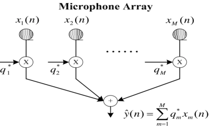
(26) 1.2 Overview of Beamformers The second stage of the general speech enhancement system is a beamformer which deals with the suppression of interference signals and environmental noises. Normally, a beamformer (i.e., spatial filter) which uses the spatial information can generate directionally sensitive gain patterns that can be adjusted to increase sensitivity to the speaker of interest and decrease sensitivity in the direction of competing sound sources, interference signals and environmental noises. Consequently, beamformer can suppress undesired speech signals and enhance desired speech signals at the same time. For a narrowband assumption, a beamformer is a linear combiner that produces an output by weighting and summing components of the snapshot of the received data, i.e. M. yˆ ( n ) = ∑ q m* x m ( n ) = q H x ( n ). (1-1). m =1. where. x (n ) is the snapshot of the received data, the superscript H denotes the. Hermitian operation, and q is the filter coefficient vector given by q = [q1 L q M ] . T. The diagram is shown in Fig. 1.4.. x2 ( n ). x1 ( n ). q 1*. x M (n ). q2*. * qM. yˆ ( n ) =. M. ∑q m =1. Figure 1-4 Diagram of the beamformer. 6. * m. xm ( n ).

(27) However, the application in which microphone array is used is different from that of conventional array applications. This is because the speech signal has an extremely wide bandwidth relative to its center frequency. Therefore, the conventional narrowband beamformer is not suitable. Generally, for broadband signals or speech signals, a finite impulse response (FIR) filter is used on each microphone and the filter outputs are summed to generate a single-channel enhanced speech signal. For example, if a microphone array contains M microphones, each including a P taps filter, then there are MP free filter coefficients in time-domain wide-band beamformer architectures. Existing beamformers may be approximately divided into four categories: fix-coefficients beamformers, post-filtering beamformers, subspace beamformers, and adaptive beamformers.. 1.2.1. Fix-coefficients beamformers. The first category called fix-coefficients beamformers including constant directivity beamformer (CDB) [28-32] and superdirective beamformers [33-36], utilizes fixed coefficients to achieve a desired spatial response. CDB is designed to keep a constant beampattern over the all frequency bins of interest, e.g., the spatial response is approximately the same over a wide frequency band. The drawback of CDB is that the size of the microphone array is related to the lowest frequency bin and the number of microphone is relatively high. Consequently, for speech recognition applications, CDB and is impractical. Unlike CDB, superdirective beamformer attempts to minimize the power of the filtered output signal yˆ ( n ) while keeping an undistorted signal response in the desired location with a finite array size. Moreover, the noise information, such as the noises’ locations and noises’ models can be included to improve the noise 7.

(28) suppression performance. Fix-coefficient beamformers generally assume the desired sound source, interference signals, and noises are slowly varying and at a known location. Therefore, these algorithms are sensitive to steering errors which limit their noises suppression performance and cause the desired signal distortion or cancellation. Furthermore, these algorithms have limited performance at enhancing a desired signal in highly reverberation environments.. 1.2.2. Post-filtering beamformers. To enhance the noise suppression performance, post-filtering techniques [37-40] have been proposed. Post-filtering techniques perform post-processing to the filtered output signal yˆ ( n ) by using a single channel filter, such as the Wiener filter and the normalized least mean square (NLMS) adaptation criterion. Notably, the filtered output signal is derived from a beamformer, including CDB, superdirective beamformer, and so on. Consequently, if the desired signal distortion or cancellation exists in the filtered output signal, the distortion or cancellation cannot be avoided even with a post-filtering beamformer.. 1.2.3. Subspace beamformers. Subspace beamformers [41-44] [126-127] are developed based on the form of the optimal multidimensional Wiener filter. These algorithms utilize generalized singular value decomposition (GSVD) or singular value decomposition (SVD) to decompose the correlation matrix of the desired signal and the received signal when the desired signal cannot be observed. Because of the unobservable desired signal, these beamformers cannot deal with the channel distortion directly.. 8.

(29) 1.2.4. Adaptive beamformers. Instead of using fixed coefficients to suppress noises and interference signals, an adaptive beamformer [45-64] can adaptively forms its directivity beampattern to the desired signal and its null beampattern to the undesired signals. In the fix-coefficients beamformers, the null beampattern only exits when the noise’s direction is known and remains unchanged. Adaptive beamformers can release this limitation and perform a better noise suppression performance than fix-coefficient beamformers. Although an adaptive beamformer can adapt itself to the change of environmental noises, the steering errors caused by microphone mismatch or DOA estimation errors deteriorate the performance. To develop a robust adaptive beamformer to cope with the steering errors is still an important issue in this field.. 1.3 Outline of Proposed System Figure 1-5 shows the block diagram of the proposed reference-signal-based speech enhancement system, which contains three main components: voice activity detection (VAD) algorithm, robust reference-signal-based speaker’s location detection algorithm, and reference-signal-based frequency-domain adaptive beamformer.. M. M. M. Figure 1-5 Block diagram of proposed reference-signal-based speech enhancement system. 1.3.1. VAD Algorithm 9.

(30) An important issue in many speech processing applications is the determination of presence of speech segments in a given sound signal. To deal with this requirement, VAD was developed to detect silent and speech intervals. In the proposed reference-signal-based speech enhancement system, the VAD result drives the overall system to switch between two operational stages, the silent stage and the speech stage. Therefore, this first component in the proposed system is to provide an accurate silence detection mechanism. Figure 1-6 illustrates the flowchart of the fundamental VAD algorithm which is a two-step procedure: feature extraction and classification method.. Figure 1-6 Flowchart of the fundamental VAD algorithm. Feature Extraction: Relevant features are extracted from the speech signal. To achieve a good detection of speech segments, the chosen features have to show a significant variation between speech and non-speech signals.. Classification Method: In general, a threshold is applied to the extracted features to distinguish between the speech and non-speech segments. The threshold can be a fixed value or an adjustable value. Moreover, decision rules using statistical properties [65-66] were also implemented to deal with the classification problem. These features normally represent the variations in energy levels or spectral difference between noise and speech. There exist many discriminating features in speech detection, such as the signal energy [67-69], LPC [70-71], zero-crossing rates [72], the entropy [73-75], and pitch information [76]. Various features or feature vector, 10.

(31) the combinations of features, have been adopted in VAD algorithms [77-78]. To adapt to the changes of environmental noises or various noise characteristics, noise estimation method during non-speech periods should be added into the fundamental VAD algorithm [79-80]. The algorithm [81] is evaluated in Chapter 6 under vehicular and indoor environments. Based on the experimental results, the VAD algorithm in [81] is suitable for implementing the proposed reference-signal based speech purification system.. 1.3.2. Reference-signal-based Speaker’s Location Detection Algorithm. Because conventional sound source localization algorithms suffer from the uncertainties of environmental complexity and noise, as well as the microphone mismatch, most of them are not robust in real practice. Without a high reliability, the acceptance of speech-based HCI would never be realized. This dissertation presents a novel reference-signal-based speaker’s location detection approach and demonstrates high accuracy within a vehicle cabinet and an office room using a single uniform linear microphone array. Firstly, to perform single speaker’s location detection, the proposed approach utilize Gaussian mixture models (GMM) to model the distributions of the phase differences among the microphones caused by the complex characteristic of room acoustic and microphone mismatch. The individual Gaussian component of a GMM represents some general location-dependent but content and speaker-independent phase difference distributions. Moreover, according to the experimental results in Chapter 6, the scheme performs well not only in non-line-of-sight cases, but also when the speakers are aligned toward the microphone array but at difference distances from it. This strong. 11.

(32) performance can be achieved by exploiting the fact that the phase difference distributions at different locations are distinguishable in a non-symmetric environment. However, because of the limitation of VAD algorithm, an unmodeled speech signal might trigger the algorithm and drive the system to a wrong stage. This unexpected signal, which is not emitted from one of the modeled locations, may come from radio broadcasting of the in-car audio system and the speaker’s voices from unmodeled locations. Therefore, this dissertation proposes a threshold adaptation method to provide high accuracy in locating multiple speakers and robustness to unmodeled sound source locations.. 1.3.3. Reference-signal-based Frequency-Domain Beamformer. This dissertation proposes two frequency-domain beamformers based on reference signals. They are soft penalty frequency-domain block beamformer (SPFDBB) and frequency-domain adjustable block beamformer (FDABB). Compared with the conventional reference-signal-based time-domain adaptive beamformers using NLMS adaptation criterion, these frequency-domain methods can significantly reduce the computational. effort. in. speech. recognition. applications.. Like. other. reference-signal-based techniques, SPFDBB and FDABB minimize microphone mismatch, desired signal cancellation caused by reflection effects and resolution due to the array’s position. Additionally, these proposed methods are appropriate for both near-field and far-field environments. Generally, the convolution relation between channel and speech source in time-domain cannot be modeled accurately as a multiplication in the frequency- domain with a finite window size, especially in speech recognition applications. SPFDBB and FDABB can approximate this multiplication by treating several frames as a block to achieve a better beamforming result. Moreover, 12.

(33) FDABB adjusts the number of frames in a block on-line to cope with the variation of characteristics in both speech and interference signals. In Chapter 6, a better performance is found to be achievable by combining SPFDBB or FDABB with a speech recognition mechanism. For a speech recognition application, another important issue in real-time beamforming of microphone arrays is the inability to capture the whole acoustic dynamics via a finite-length of data and a finite number of array elements. For example, the source signal coming from the side-lobe through reflection presents a coherent interference, and the non-minimal phase channel dynamics may require an infinite data to achieve perfect equalization (or inversion). All these factors appear as uncertainties or un-modeled dynamics in the receiving signals. Therefore, the proposed system attempts to adopt the H∞ adaptation criterion, which does not require a priori knowledge of disturbances and is robust to the modeling error in a channel recovery process. The H∞ adaptation criterion is to minimize the worst possible effects of the disturbances including modeling errors and additive noises on the signal estimation error. Consequently, using the H∞ adaptation criterion can further improve the recognition performance. It should be emphasized that DOA and beamformer are generally treated as two independent components and discussed respectively in general speech enhancement systems. However, the proposed reference-signal-based speaker’s location detection algorithm and frequency-domain beamformer can be potentially integrated because they perform in the same operational architecture. Please refer to Chapter 7 for more detail.. 13.

(34) 1.4 Contribution of this Dissertation The contribution of this dissertation is to propose and implement innovative algorithms for sound source localization and speech purification. Although a considerable number of studies have been made on these two fields over the past 40 years, only few attempts have so far been made at simultaneously targeting on practical issues such as microphone mismatch, near-field and far-filed, channel dynamics recovery, desired signal cancellation, and the resolution effect for speech purification. Further, for the sound source localization, important issues in practice are the non-line-of-sight and line-of-sight, reverberation, microphone mismatch, and noisy environment. This dissertation proposes two frequency domain beamformers, namely SPFDBB and FDABB, and speaker’s location detection approach to simultaneously overcome the issues mentioned above. 1. SPFDBB and FDABB can flexibly adjust the emphasis on the channel dynamics recovery and noise suppression. Moreover, SPFDBB and FDABB reduce the computational effort significantly, and deal with the problem that the convolution relation between channel and speech source in time-domain cannot be modeled accurately as a multiplication in the frequency domain with a finite window size. 2. To cope with the variation of room acoustics, a frame number adaptation method is proposed using an index named CBVI in FDABB. 3. An H∞ adaptation criterion is applied to the proposed SPFDBB and FDABB to reduce the effect of modeling error, which is common in the adaptive beamformers. 4. The proposed multiple speakers’ locations detection approach is able to provide the suitable length of testing sequences and thresholds. Therefore, it can obtain the high. 14.

(35) accuracy on detecting speaker’s location and reduce the error caused by unmodeled locations and the overlapped speech segments.. 1.5 Dissertation Organization This chapter provides a brief introduction to the general microphone-array-based speech enhancement system, including the overviews of DOA algorithms, and beamformers. This chapter also briefly discusses three main components in the proposed reference-signal-based speech enhancement system. Chapter 2 introduces the reference-signal-based time-domain adaptive beamformer using NLMS adaptation criterion. Chapter 3 presents SPFDBB and FDABB using NLMS adaptation criterion and analyzes the computational efforts of the two proposed frequency-domain and the time-domain beamformers. Chapter 4 studies the robustness of the H∞ adaptation criterion. Chapter 5 presents the proposed reference-signal-based speaker’s location detection approach for single speaker’s and multiple speakers’ locations detection. Chapter 6 shows the simulation as well as the experimental results in real environment. Chapter 7 gives some concluding remarks and avenues for future research.. 15.

(36) Chapter 2 Reference-signal-based Time-domain Adaptive Beamformer. 2.1 Introduction Speech enhancement systems are now becoming increasingly important, especially with the development of automatic speech recognition (ASR) applications. Although various solutions have been proposed to reduce the desired signal cancellation, particularly desired speech, in noisy environments, the recognition rate is still not satisfactory. Earlier approaches, such as delay-and-sum (DS) beamformer [82], Frost beamformer [45], and generalized sidelobe cancellation (GSC) [46], are only good in ideal cases, where the microphones are mutually matched and the environment is a free space. The causes of performance degradation include array steering vector mismodeling due to imperfect array calibration [47], and the channel effect (e.g., near-field or far-field problem [83], environment heterogeneity [84] and source local scattering [85]). To manage these limitations, the most common linearly constrained minimum variance (LCMV)-based techniques [33] and [57] have been developed to reduce uncertainty in the sound signal’s look direction. However, these approaches are 16.

(37) limited by scenarios with look direction mismatch. Henry [58] employed the white noise gain constraint to overcome the problem of arbitrary steering vector mismatch. Unfortunately, no clear guidelines are available for choosing the parameters. Hoshuyama et al. [59] proposed two robust constraints on blocking matrix design. Cannot et al. [86] proposed a new channel estimation method for standard GSC architecture in the frequency domain, but loud noises, and in particular circuit noise, would heavily degrade its channel estimation accuracy. Sergiy A. et al. [60] proposed an approach based on optimizing the worst-case performance to overcome an unknown steering vector mismatch. However, a worst case is defined as a small random perturbation, which may not suitable for general cases. Dahl et al. [61] proposed the reference-signal-based time-domain adaptive beamformer using NLMS adaptation criterion to perform indirect microphone calibration and to minimize the speech distortion due to the channel effect by using pre-recorded speech signals and a reference signal. Moreover, Yermeche et al. [62] and Low et al. [63] also utilized the reference signal to estimate the source correlation matrix and calibration correlation vector. These methods in [61-63] are fundamentally the same except that the works in [62-63] do not require a VAD. However, VAD is useful for finding speaker’s location and enabling the speech purification system and speech recognizer. Therefore, the methods in [62-63] cannot offer any profit in ASR applications. The. following. section. describes. the. system. architecture. of. the. reference-signal-based time-domain adaptive beamformer and the corresponding dataflow. It also presents how to derive the pre-recorded and reference signals. Finally, conclusions are given in Section 2.3.. 17.

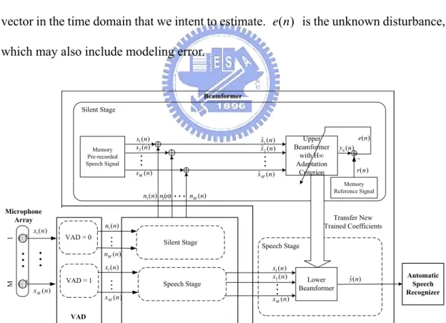
(38) 2.2 System Architecture The architecture of the reference-signal-based time-domain adaptive beamformer is shown in Fig. 2-1. A speech signal passing through multi-acoustic channels is monitored at spatially separated sensors (a microphone array). Two kinds of signals, the pre-recorded signal, {s1 ( n ) L s M ( n )} , and the reference signal, r (n ) , are necessary before executing the reference-signal-based time-domain adaptive beamformer. Let M denotes the number of microphones. A set of pre-recorded speech signals are collected by placing a loudspeaker or a person in the desired position, and by letting the loudspeaker emit or the person speak a short sentence when the environment is quiet. Therefore, the pre-recorded speech signals provide a priori information between speakers and the microphone array. Additionally, the reference signal is acquired from the original speech source that emitted from the loudspeaker or using another microphone located near the person to record the speech. In practice, the loudspeaker or the person should move around the desired position slightly to obtain an effective recording. For example, Fig. 2-2 illustrates a vehicular environment with a headset microphone and a microphone array. The person is right on the desired location and speaks several sentences when the environment is quiet. The sentences are simultaneously recorded by the headset microphone and the microphone array. The speech signal collected by the headset microphone and the microphone array are called the reference signal and pre-recorded speech signals individually. Notably, the user does not need the headset microphone during the online applications. After collecting the pre-recorded speech signals and the reference signal, the complete procedures of the reference-signal-based time-domain beamformer are divided in two stages, the silent stage and the speech stage, through the result of VAD algorithm. 18.

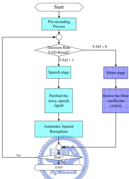
(39) s1 (n) s2 ( n). xˆ1 ( n ) xˆ 2 ( n). M. M. sM (n). M. x1 ( n ). M M x M (n ). r (n). xˆ M ( n). n1 (n) n2(n). e(n) yb (n). nM (n). n1 (n). M. nM (n). x1 ( n ). x1 ( n ) x2 ( n ). M. yˆ (n). M. x M (n ). xM (n ). Figure 2-1 System architecture of the reference-signal-based time-domain adaptive beamformer. Figure 2-2 Installation of the array and headset microphone inside a vehicle. In other words, the VAD result decides whether to switch the system to the silent stage or speech stage. First, if VAD result equals to zero which means no speech signal contains in the received signals, {x1 ( n ) L x M ( n )} (i.e. the received signals are totally environmental noises denoted as {n1 ( n ) L n M ( n )} ), then the system is switched to the first stage: the silent stage. Given that the environmental noises are assumed to be additive, the acoustic behavior of the speech signal received when a 19.

(40) speaker is talking in a noisy environment can be expressed as a linear combination of the pre-recorded speech signal and the environmental noises. Therefore, in this stage, the system combines the online recorded environmental noise, {n1 ( n ) L n M ( n )} , with the pre-recorded speech database, {s1 ( n ) L s M ( n )} , to construct the training signals, {xˆ1 ( n ) L xˆ M ( n )}, and to performs NLMS adaptation criterion to derive the filter coefficient vectors. Notably, the filter coefficient vectors are updated via the reference signal and the training signal thus implicitly solving the calibration. Secondly, if the received sound signal is detected as containing speech signal, then the system is switched to the second stage, called speech stage. In this stage, the filter coefficient vectors obtained by the first stage are applied to the lower beamformer to suppress noises and enhance the speech signal in the speech stage. Finally, the single-channel purified speech signal yˆ ( n ) is transformed to the frequency domain and then sent to the automatic speech recognizer. Because the variation between pre-recorded speech signals and the reference signal contains useful information about the dynamics of channel, electronic equipments uncertainties, and microphones’ characteristics, the method potentially outperforms other un-calibrated algorithms in real applications. Figure 2-3 presents the flowchart of the reference-signal-based time-domain adaptive beamformer.. 20.

(41) Figure 2-3 Flowchart of the reference-signal-based time-domain adaptive beamformer While the speaker in the desired location is silent, the formulation of referenced-signal-based time-domain beamformer can be expressed as the following linear model:. r( n) = q T xˆ ( n) + e( n) = q T (s( n) + n( n)) + e( n). (2-1). where the superscripts T denotes the transpose operation and e( n) is the error signal in the time domain. Notice that italics fonts represent scalars, bold italics fonts represent vectors, and bold upright fonts represent matrices in this dissertation. Let the parameter P denote the FIR taps of the each estimated filter, and then 21.

(42) s( n) = [s1 ( n) L s M ( n)]. T. denotes the pre-recorded signal vector;. n( n) = [n1 ( n) L nM ( n)]. T. denotes the MP × 1 online recorded environmental. noise vector; T xˆ ( n) = [xˆ1 ( n) L xˆ M ( n)]. denotes. the. MP × 1. training. signal. vector;. q = [q1 L q M ] denotes the MP × 1 filter coefficient vector of the time-domain T. beamformer that we intent to estimate. The corresponding vectors of the signals defined above are,. xˆ i ( n) = [xˆi ( n) L xˆ i ( n − P + 1)] ; si ( n) = [si ( n) L si ( n − P + 1)] ; ni ( n ) = [ni ( n ) L ni ( n − P + 1)] ; qi = [qi1 L qiP ] . The well-known normalized LMS solution obtained by minimizing the power of error signal is represented in Eq. (2-2). q( n + 1) = q( n ) +. xˆ ( n ) e( n ) γ + xˆ ( n ) T xˆ ( n ). (2-2). where γ is a small constant included to ensure that the update term does not become excessively large when xˆ ( n )T xˆ ( n ) temporarily become small. The purified signal can be calculated by. yˆ ( n ) = x T ( n )q( n ). (2-3). where x ( n ) = [x1 ( n ) L x M ( n )] is the MP ×1 online recorded noisy speech T. signal vector acquired by the microphone array, and. x i ( n ) = [x i ( n ) L x i ( n − P + 1)] .. 22.

(43) 2.3 Summary This chapter presents the reference-signal-based system architecture which implicitly contains the information of the channel effect and microphones’ characteristics. This architecture implicitly obtains the acoustic behavior from the desired location to microphone array and reduces the efforts of directly performing microphone calibration and channel inversion. Furthermore, it can be applied on both near-field and far-field situations which offers a significant advantage in speaker localization and beamformer algorithms. Extension of this idea to further improve the ASR rates will be described in the following chapters. Moreover, a novel speaker’s location detection algorithm based on the reference-signal-based architecture is also proposed.. In. addition,. Chapter. 6. compares. the. performance. of. the. reference-signal-based time-domain adaptive beamformer and other well-known non-reference-signal-based beamformers to show the effectiveness of the proposed method.. 23.

(44) Chapter 3 Reference-signal-based Frequency-domain Adaptive Beamformer. 3.1 Introduction The required computational effort could be large when applying a large FIR filter coefficients, e.g., 256 to 512 taps in the time-domain adaptive beamformer introduced in the previous chapter. For subsequent ASR operation, another effort to compute Discrete Fourier transform (DFT) is required. One possible way to simplify the computational complexity is to compute the beamformer directly in the frequency domain because ideally the large FIR taps can be replaced by a simple multiplication at each frequency bin (e.g., the FIR filter with dimension of MP × 1 is represented by filter coefficient vector M × 1 in the frequency domain where. M. is the. microphone number and P denotes the FIR taps). Moreover, the purified speech signal after a frequency-domain beamformer can be sent directly to the ASR. As explained later in this chapter and Chapter 6, the saving of computational effort is quite significant.. 24.

(45) In a reference-signal-based beamformer, coefficients adjustment has two objectives: to minimize the interference signal and noises, and to equalize the channel effect (e.g. room acoustics). Channel equalization is important for ASR since the channel distortion may greatly reduce the recognition rate. By formulating the same problem in the frequency domain, channel distortion can be emphasized using a priori information. In this chapter, a penalty function is incorporated into the performance index to calculate the filter coefficient vectors. This proposed algorithm is called SPFDBB. A real-time frequency-domain beamformer is necessary to apply the short time Fourier transform (STFT). However, the corresponding window size of the STFT has to be fixed by the training data settings in ASR. For an environment with longer impulse response duration, the convolution relation between channel and speech source in time-domain cannot be modeled accurately as a multiplication in the frequencydomain with a finite window size. Therefore, the finite window size may not provide enough information for the coefficient adjustment and could not fit the assumptions that filter coefficient vector and the error signal should be independent to the input data in the NLMS adaptation criterion. In this case, SPFDBB takes the frame average over several frames as a block to improve the approximation of the linear model shown in Eq. (2-1). In other words, a block of windowed data is simultaneously adopted to calculate the filter coefficient vectors in the SPFDBB algorithm. The number of frames in a block is denoted as the frame number L . Intuitively, a large frame number could enhance the accuracy of the filter coefficient estimation. However, if the room acoustic dynamic changes suddenly, the channel response is difficult to be adjusted quickly when taking a large frame number for the updating process. Furthermore, the requirement of the length of the processed data would be too large when a large value 25.

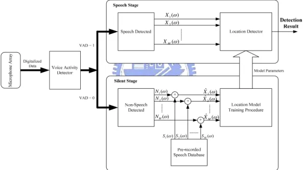
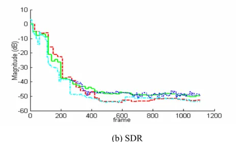
(46) of L is chosen. Therefore, SPFDBB is further enhanced by allowing the frame number to be adapted on-line. A novel index called changing block values index ( CBVI ) is defined as the basis for adjusting the frame number. The overall algorithm is called FDABB. The remainder of this chapter is organized as follows. Section 3.2 describes the system architecture and the corresponding dataflow. Section 3.3 represents SPFDBB, one of the reference-signal-based frequency-domain adaptive beamformers which utilizes NLMS adaptation criterion. Section 3.4 introduces the other proposed method, FDABB, and also analyzes the computing efforts of SPFDBB, FDABB and the reference-signal-based time-domain beamformer. Two frequency-domain performance indexes, the source distortion ratio (SDR) and the noise suppression ratio (NSR) are defined in Section 3.5. Finally, conclusions are given in Section 3.6.. 3.2 System Architecture Figure 3-1 shows the overall system architecture. The pre-recorded speech signals, S1 (ω, k ),L, S M (ω, k ) , and the reference signal, R(ω, k ) , can be recorded by the same way described in Chapter 2 when the environment is quiet. After acquiring the pre-recorded speech signal and the reference signal, the overall system automatically executes between the silent and speech stages based on the VAD result. If the result of VAD equals to zero which means no speech signal contained in the received signal, {x1 ( n ) L x M ( n )}, then the system is switched to the silent stage in which the adaptation of FDABB or SPFDBB is turned on. The filter coefficient vectors of FDABB or SPFDBB are adjusted through NLMS adaptation criterion in this stage. Notably, SPFDBB is a part of FDABB and can be executed separately. 26.

(47) On the other hand, if the received sound signal is detected as containing speech signal, then the system is switched to the second stage called speech stage. In this stage, the filter coefficient vectors obtained in the silent stage are applied to the lower beamformer to suppress the interference signals and noises, and enhance the speech signal. Finally, the purified speech signal Yˆ (ω, k ) is directly sent to the ASR.. ε x (ω, k ) ε s (ω, k ) Xˆ 1 (ω, k ) Xˆ 2 (ω, k ). S1 (ω, k ) S2 (ω, k ). M. M. S M (ω, k ). Xˆ M (ω, k ). M. N1 (ω, k ) N 2 (ω, k ). x1 ( n ). M M x M (n ). Yb (ω, k ) R(ω, k ). N M (ω, k ). N1 (ω, k ). M. N M (ω, k ) X 1 (ω, k ). X 1 (ω, k ) X 2 (ω, k ). M. Yˆ (ω, k ). M. X M (ω, k ). X M (ω, k ). Figure 3-1 Overall system structure. 3.3 SPFDBB Using NLMS Adaptation Criterion The linear model in Eq. (2-1) is transformed to the frequency domain by padding the short-time Fourier transform of the error signal with zeros to make it twice as long as the window length. The error signal at frequency ω and frame k is written as:. ε x (ω , k ) = R (ω , k ) − Q H (ω , k ) Xˆ (ω , k ). 27. (3-1).

(48) where R(ω, k ) is the reference signal in the frequency domain, Q (ω , k ) denotes the. [. ]. T filter coefficient vector we intend to find, and Xˆ (ω, k ) = Xˆ 1 (ω, k ) L Xˆ M (ω, k ). is the training signal vector at frequency ω and frame k . The optimal set of filter coefficient vectors can be found using the formula: min ε x (ω, k )ε x (ω, k ) *. Q. [. ][. ]. * = min R(ω, k ) − Q H (ω ) Xˆ (ω, k ) R(ω, k ) − Q H (ω ) Xˆ (ω, k ) Q. (3-2). where the superscripts ∗ denotes the complex conjugate. The normalized LMS solution of Eq. (3-2) is given by:. Q(ω, k + 1) = Q(ω, k ) +. ε x (ω, k ) Xˆ * (ω, k ) γ + Xˆ H (ω, k ) Xˆ (ω, k ). (3-3). Consequently, the purified output signal can be obtained by the following equation:. Yˆ (ω , k ) = Q H (ω , k ) X (ω , k ). (3-4). where X (ω, k ) = [ X 1 (ω, k ) L X M (ω, k )] is the received signal vector which contains speech source, interference and noise. From Eq. (3-1), the filter coefficient vector equalizes the acoustic channel dynamics and also creates the null space for the interference and noise. As mentioned above, the filter coefficient vector Q (ω, k ) equalizes the channel response and rejects interference signals and noises. To emphasize these two objectives differently, a soft penalty function is added into the performance index as,. 28.

(49) min ε x (ω, k )ε x (ω, k ) + με s (ω, k )ε s (ω, k ) *. *. Q. (3-5). where μ is the soft penalty parameter and. ε s (ω, k ) = R(ω, k ) − Q H (ω, k ) S (ω, k ). (3-6). Then, the iterative equation utilizing the NLMS adaptation criterion can be shown as:. Q (ω, k + 1) = Q (ω, k ) +. λ {G x (ω, k ) + μG s (ω, k )} γ + X (ω, k ) X (ω, k ) + μS H (ω, k ) S (ω, k ) H. (3-7). where G x (ω, k ) = ε x (ω, k ) Xˆ * (ω, k ) , G s (ω, k ) = ε s (ω, k ) S * (ω, k ) and λ is the step size. If. the soft penalty is set to infinity, then the system only focuses on minimizing the channel distortion. On the other hand, the system returns to the formulation in Eq. (3-2) when the soft penalty is set to zero. The problem of Eq. (3-7) is the window size has to equal that in ASR to ensure calculation accuracy. However, the window size may be too small for cases where the acoustic channel response duration is long (e.g., long reverberation path). Because the perturbation caused by channel model error is highly correlated to the reference signal instead of the uncorrelated noise, the updating process will not converge to a fixed channel response which is shown in Fig 6.3 and the relation between two sequential frames is highly relative. Taking the frame average over several frames (denoted as L ) allows the channel response to be approximated; since information of channel response which is not contained in one frame could be regarded as an external noise in the next frame. Thus, the performance index can be written in a quadratic from as: 29.