使用Lagrangean 近似方法建立具有服務品質之點對點虛擬路徑

全文

(1)國立交通大學資訊工程系碩士論文. 使用 Lagrangean 近似方法建立具有服務品質之點對點虛擬路徑. Construct QoS end-to-end virtual path using Lagrangean relaxation method. 研究生：劉名恕指導教授：陳昌居. 博士. 中華民國九十三年五月. I.

(2) Construct QoS end-to-end virtual path using Lagrangean relaxation method. 研究生：劉名恕. Student：Ming-Su Liu. 指導教授：陳昌居. Advisor：Chang-Jiu Chen. 國立交通大學資訊工程學系碩士論文. A Thesis Submitted to Department of Computer Science and Information Engineering College of Electrical Engineering and Computer Science National Chiao Tung University in partial Fulfillment of the Requirements for the Degree of Master in Computer Science and Information Engineering June 2004. Hsinchu, Taiwan, Republic of China. 中華民國九十三年六月. II.

(3) 使用 Lagrangean 近似方法建立具有服務品質之點對點虛擬路徑研究生：劉名恕. 指導教授：陳昌居國立交通大學資訊工程學系摘要. 在現今的網路設計當中中,越來越重視 QoS (Quality of Service)的重要性,在我們的設計中,我們針對不同服務所需滿足之服務要求(在文章中我們關心的目標是以每一個連線的點對點的延遲為訴求), 我們的問題是專注在滿足各個連線的服務品質要求下, 尋找一種路由的方式, 建立虛擬路徑, 使得使用率最高的連結上的負載為最輕 (Load Balance Model), 此種構想是希望滿足現有的連線的需求之下, 尋找一種資源分配的方式, 去保留最富彈性的資源選擇給後續再進入網路中要求建立虛擬路徑的連線, 使得其有最大的選擇空間。我們將此問題規劃成為 mixed non-linear programming 的形式, 我們利用 Lagrangean Relaxation 的方式去將此問題的複雜度降低(將某些限制放寬), 再利用此放寬限制後的問題的結果作為一個指引, 搭配我們所提出的一種近似最佳化演算法, 尋得一組合法的解答, 再利用 subgradient 的方式,去一直改進答案的優良性,我們的目標是雖然我們無法得到真正的最佳解, 但我們能藉由此種方法的下限值與上限值的差距, 經由實驗的數據, 可以得知我們的方法已經非常優秀, 幾乎求得最佳值。. III.

(4) Construct QoS end-to-end virtual path using Lagrangean relaxation method Student : Ming-Su Liu Advisor : Dr. Chang-Jiu Chen Department of Computer Science and Information Engineering National Chiao-Tung University. Abstract In this thesis, we have improved a QoS routing problem. We give an approach to minimize the congested link utilization while to satisfy individual connection’s packet delay. We use a Lagrangean Relaxation based approach augmented with an efficient primal heuristic algorithm, called Lagrangean Relaxation Heuristic (LRH). With the aid of generated Lagrangean multipliers and lower bound indexes, the primal heuristic algorithm of LRH achieves a near-optimal upper-bound solution. A performance study delineated that the performance trade-off between accuracy and convergence speed can be manipulated via adjusting the Unimproved Count (UC) parameter in the algorithm. We have drawn comparisons of accuracy and computation time between LRH and the Linear Programming Relaxation (LPR)-based method, under three networks named NSFNET, PACBELL, and GTE and three random networks. Experimental results demonstrated that the LRH is superior to the other approach, namely the LPR method, in both accuracy and computational time complexity, particularly for larger size networks. IV.

(5) 誌. 謝. 進入研究所兩年,受到學長與老師們許多的照顧,也能從學長與老師們做事的方法上, 訓練自己獨立思考的能力,在這裡要特別感謝幫助過我的人,而實驗室的和諧氣氛也讓我能更加融入團體中,大家一起的歡笑與淚水都帶給我很多美好的回憶,也感謝爸爸媽媽無微不至的照顧,讓我能專心於課業上,感謝這一路上走來,陪伴我的所有朋友,謝謝大家!!. V.

(6) Contents 摘要 .................................................................................................................................... III Abstract.............................................................................................................................. IV 誌. 謝 ................................................................................................................................ V. Contents ............................................................................................................................. VI List of Figures.................................................................................................................... VI List of Tables.....................................................................................................................VII 1.. Introduction................................................................................................................10. 2.. Previous Work............................................................................................................13 2.1. Source Routing Algorithms ....................................................................................13 2.2. Distributed Routing Algorithms .............................................................................16 2.3. Hierarchical Routing Algorithms...........................................................................19 2.4. Previous Work Summary ........................................................................................21. 3.. Problem Model and Formulation .............................................................................22 3.1. Problem Description ...............................................................................................22 3.2. Network Model and Definition...............................................................................23 3.3. Problem Formulation .............................................................................................24. 4.. Lagrangean Relaxation and Problem Decomposition ............................................30 4.1. Solving Subproblem 1 .............................................................................................32. VI.

(7) 4.2. Solving Subproblem 2 .............................................................................................33 4.3. Solving Subproblem 3 .............................................................................................34 4.4. Subgradient Optimization Procedure .....................................................................37 4.5. Summary of Lagrangean Relaxation Method .......................................................39 5.. Lagrangean-based Heuristic Algorithm ..................................................................40 5.1. Proposed Lagrangean-based Heuristic A lgorithm ...............................................41 5.2. Evaluation of the Feasible Schedule......................................................................42. 6.. Experimental Results.................................................................................................43 6.1. Performance Study..................................................................................................44 6.2. Performance Comparisons .....................................................................................46. 7.. Conclusions and Future Works ................................................................................55. Reference ............................................................................................................................58. VII.

(8) List of Figures FIGURE 1 AN EXAMPLE OF PNNI ROUTING ........................................................................21 FIGURE 2 THE ALGORITHM OF SUBPROBLEM 1..................................................................33 FIGURE 3 THE ALGORITHM OF SUBPROBLEM 2..................................................................34 FIGURE 5 THE ALGORITHM OF SUBPROBLEM 3..................................................................37 FIGURE 6 THE ALGORITHM OF UPDATE-STEP-SIZE AND UPDATE-MULTIPLIER ..................39 FIGURE 7 THE ALGORITHM OF LRM..................................................................................40 FIGURE 8 THE ALGORITHM OF LRM EVALUATION PROCEDURE ......................................42 FIGURE 9 THE ALGORITHM OF PRIMAL-HEURISTIC ..........................................................43 FIGURE 10 CONVERGENCE SPEED VERSUS ACCURACY ON THE BASIS................................45 FIGURE 11 THREE NETWORKS ............................................................................................48 FIGURE 12 THREE RANDOM GENERATING NETWORKS. .....................................................52 FIGURE 13 COMPARISON OF ACCURACY UNDER THREE RANDOM NETWORKS. .................53 FIGURE 14 COMPARISON OF COMPUTATION TIME UNDER THREE RANDOM NETWORKS. ..54. VIII.

(9) List of Tables TABLE 1 UNICAST ROUTING ALGORITHMS .........................................................................22 TABLE 2 NUMERICAL RESULTS FOR NSFNET NETWORK .................................................49 TABLE 3 NUMERICAL RESULTS FOR PACBELL NETWORK ...............................................49 TABLE 4 NUMERICAL RESULTS FOR GTE NETWORK .........................................................49. IX.

(10) 1.. Introduction To ensure reliable and high-quality network services, routing and capacity assignment. policies should be carefully designed. Traditional quasi-static routing algorithms attempt to optimize a certain aggregate measure, e.g. to minimize the average end-to-end packet delay [3, 15]. However, this kind of performance measures may not be consistent with the service objectives and may result in fairness problems. Since end-to-end performance in users’ straightforward perception about the service quality, service objectives are typically specified on an end-to-end basis for many new services, e.g. Switched Multi-megabit Data Service (SMDS), Frame Relay Service (FRS). Asynchronous Transfer Mode (ATM) and Advanced Intelligent Network (AIN). As such, from service providers’ perspective, it is more appropriate to design a routing and capacity assignment policy such that end-to-end quality of service for each user is satisfied than a policy to optimize an aggregate performance measure, which in many cases may result in good average performance but unacceptable performance for some users (fairness issues). To ensure user-perceived end-to-end QoS requirement is one of the most important issues in providing modern network services, which typically requires sophisticated design of routing and capacity management policies. User-perceived end-to-end QoS measures include, for example, mean packet delay, packet delay jitter and packet loss probability. Besides users’ perspective of QoS, from the service providers’ perspective (which is a 10.

(11) traditional view of network performance management), optimizing a certain system-level performance measure, e.g. overall network utilization or average cross-network delay among all users, or call blocking probability is another major concern, Unfortunately, these two perspectives/objectives may not be entirely agreeable with each other. This then places a major challenge to network managers and therefore calls for an integrated methodology to consider these perspectives in a joint fashion. The routing problem in virtual circuit networks has been a traditional research topic in computer networks and has attracted even more attention since the emergence of the Asynchronous Transfer Mode (ATM) technology. However, most previous researches on virtual circuit routing considers the objective function of minimizing the average end-to-end packet delay [3, 8, 17], which address a system-optimization perspective without taking individual users into account. And also these researches do not consider the later connections, that is these current established connections may cause big load for connections that request to establish virtual circuits later. In [13] Cheng and Lin took a user-optimization approach and considered a fairness issue by minimizing the maximum individual end-to-end packet delay in virtual network, but they didn’t consider the system’s perspective. In this thesis, we attempt to jointly consider both system’s and user’s perspectives, and keep maximum tolerance to the later connections. More precisely, we construct the network into load balance model subject to end-to-end packet delay. 11.

(12) constraints for each individual user. The problem has been shown to be NP-complete which means no polynomial time algorithm for it unless P=NP. For the sake of obtaining sub-optimal solutions, Lagrangean relaxation is applied to the formulation to decompose the problem into several tractable subproblems. The candidate path set does not need to be prepared in advance and the best paths are generated while solving the subproblems in our approach. A heuristic algorithm based on the solving procedure of the Lagrangean relaxation is developed to obtain a primal feasible solution. To make a performance comparison, a linear programming based algorithm is also been developed. By examining the gap between the upper bounds obtained from Lagrangean relaxation based heuristic and linear programming to the lower bounds of Lagrangean and linear programming, it reveals that the proposed Lagrangean based algorithm can effectively and efficiently provide a near optimal solution to the QoS based routing problem in short CPU time. The remainder of this thesis is organized as follows. In Chapter 2, we first describe the problem we want to solve. In Chapter 3, a mathematical formulation of the routing problem is proposed. In Chapter 4, a solution approach to the routing problem based on Lagrangean relaxation is presented. In Chapter 5, heuristic algorithm are developed to calculate good primal feasible solutions. In Chapter 6, computational results are reported. In Chapter 7, we conclude this thesis and bring up an application based on our concept for future work.. 12.

(13) 2.. Previous Work. In this chapter, we describe the unicast source, distributed, and hierarchical routing algorithms. We explain the problems and solutions, present the existing algorithms, compare them, and discuss their pros and cons. In Table 1, we give a summarizing comparison. Algorithms are referred to by the authors’ names and a reference to their article.. 2.1.. Source Routing Algorithm. The Wang-Crowcroft Algorithm [16]-This algorithm finds a bandwidth-delay-constrained path by Dijkstra’s shortest-path algorithm. First, all links with bandwidths less than the requirement are eliminated so that any paths in the resulting graph will satisfy the bandwidth constraint. Then, the shortest path in terms of delay is found. The path is feasible if and only if it satisfies the delay constraint.. The Guerin-Orda Algorithm [19]-Guerin and Orda studied the bandwidth-constrained and delay-constrained routing problem with imprecise network states. The model of imprecision is based on the probability distribution functions. Every node maintains, for each link l, the probability pl ( w) of link l having a residual bandwidth of w units. w ∈ [0...cl ] , where cl is the capacity of the link. The goal of bandwidth-constrained routing is to find the path that has the highest probability to accommodate a new connection with a bandwidth requirement of x units. This problem can be solved by a standard shortest path algorithm with link l 13.

(14) weighted by (− log pl ( x)).. The goal of delay-constrained routing is to find a path that has the highest probability to satisfy a given end-to-end delay bound. Suppose every node maintains, for each link l, the probability pl (d ) of link l having a delay d units, where d ranges from zero to maximum possible value. It is NP-hard to find the path that has the highest probability of satisfying a given delay constraint [19], but various special cases (e.g., symmetric networks and tight constraints) can be solved in polynomial time. Heuristic algorithms were proposed for the NP-hard problem. This idea is to transform a global constraint into local constraints. More specially, it splits the end-to-end delay constraint among the intermediate links in such a way that every link in the path has equal probability of satisfying its local constraint. The heuristic then try to find the path with the best multiplicative probability over all links.. The Guerin-Orda algorithm works with imprecise information and is suitable to be used in hierarchical routing. One of the heuristic algorithms was extended by the authors to make routing based on the aggregate network state of the hierarchical model. A further study of QoS routing with imprecise state based on the probability model was done by Lorenz and Orda [6].. The Awerbuch et al. Algorithm [4]-Awerbuch et al. proposed a throughput-competitive routing algorithm for bandwidth-constrained connections. This algorithm tries to maximize the amortized (average) throughput of the network over time. It combines the function of 14.

(15) admission control and routing. Every link is associated with a cost function that is exponential to the bandwidth utilization. A new connection is admitted into the network only if there exists a path whose accumulated cost over the duration of the connection does not exceed the profit measured by the bandwidth-duration product of the connection. It was proved that such a path satisfies the bandwidth constraint. Let T be the maximum connection duration and v the number of nodes in the network. The algorithm achieves a throughput achieved by the best off-line algorithm that is assumed to know all of the connection requests in advance. The competitive routing for connections with unknown duration was studied in [5]. A survey for the competitive routing was done by Plotkin [22].. Strengths and Weaknesses of Source Routing. Source routing achieved its simplicity by transforming a distributed problem into a centralized one. By maintaining complete global state, the source node calculates the entire path locally. It avoids dealing with distributed computing problems such as distributed state snapshot, deadlock diction, and distributed termination. It guarantees loop-free routes. Many source algorithms are conceptually simple and easy to implement, evaluate, debug, and upgrade. In addition, it is much easier to design centralized heuristics for some NP-complete routing problems than to design distributed ones.. Source routing has several problems. First, the global state maintained at every node has to 15.

(16) be updated frequently enough to cope with the dynamics of network parameters such as bandwidth and delay. This makes the communication overhead excessively high for large-scale networks. Second, the link-state algorithm can only provide approximate global state due to the overhead concern and non-negligible propagation delay of state messages. As a consequence, QoS routing may fail to find an existing feasible path due to the imprecision in the global state used [1]. Third, the computation overhead at the source is excessively high. This is especially true in the case of multicast routing or multiple constraints are involved. In summary, source routing has a scalability problem. It is impractical for any single node to have access to detailed state information about all nodes and all links in a large network [19].. 2.2.. Distributed Routing Algorithms. The Wang-Crowcroft Algorithm [25]-Wang and Crowcroft proposed a hop-by-hop distributed routing scheme. Every node pre-computed a forwarding entry for every possible destination. The forwarding entry, which is updated periodically, stores the next hop on the routing path to the destination. After the forwarding entries at every node are computed, the actual routing simply follows the entries.. Given two end nodes, the path with the minimum bottleneck bandwidth is called the widest path. If there are several such paths, the one with the smallest delay is called the shortest-widest path. A link-state protocol is used to maintain complete global state at every 16.

(17) node. Based on the global state, the forwarding entry for the shortest-widest path to each destination is computed by a modified Bellman-Ford (or Dijkstra’s) algorithm [6]. A routing path is the combination of the forwarding entries indexed by the same destination at all intermediate nodes. The path is loop-free if the state information at all nodes is consistent. However, in a dynamic network the path may have a loop due to the contradicting state information at different nodes.. The Cidon et al. Algorithm [11]-The distributed multi-path routing algorithms proposed by Cidon et al. combine the process of routing and resource reservation. Every node maintains the topology of the network and the cost of every link. When a node wishes to establish a connection with certain QoS constraints, it finds a subgraph of the network which contains links that lead to destination at a “reasonable” cost. Such a subgraph is called diroute. A link is eligible if it has the required resources. Reservation messages are flooded along the eligible links in the diroute toward the destination and reserve resources along different paths in parallel. When the destination receives a reservation message, a routing path is established. The algorithm releases resources from segments of the diroute as soon as it learns that these segments are inferior to another segment. Variants of the above algorithm were proposed to make a trade-off between routing time and path optimality. Reserving resources on multiple paths makes the routing faster and more resilient to the dynamic change of network state. However, it also increases the level of resource contention. 17.

(18) The Chen-Nahrstedt Algorithm. Selective Probing [23]-Chen and Nahrstedt proposed a distributed routing framework based on selective probing. After a connection request arrives, probes are flooded selectively along those paths which satisfy the QoS and optimization requirements. Every node only maintains its local state, based on which the routing and optimization decisions are made collectively in the process of probing. As in the Shin-Chou algorithm, each probe arriving at the destination detects a feasible path.. Algorithms were derived from the framework to route connections with a variety of QoS constraints on bandwidth, delay, delay jitter, cost, and their combinations. Several techniques were developed to overcome the high communication overhead of the Shin-Chou algorithm. First, probes are only based on topological distance to the destination. Second, iterative probing is used to further reduce the overhead. At the first iteration, probes are sent only along the shortest paths. If the first iteration fails, probes are allowed to be sent along paths with increasing lengths in the following iterations. Simulation shows that with two iterations the Chen-Nahrstedt algorithm achieves substantial overhead reduction.. Ticket-Based Probing [24]-If every node maintains a global state, which is allowed to be imprecise, the ticket-based probing is used to improve the performance of selective probing. A certain number of tickets is issued at the source according to the contention level of network 18.

(19) resources. Each probe must contain at least one ticket in order to be valid. Hence, the maximum number of probes is bound by the total number of tickets, which limits the maximum number of paths to be searched. The algorithm utilizes the imprecise state at intermediate nodes to guide the limited tickets (the probes carrying them) along the best possible paths to the destination. In such a way, the probability of finding a feasible path is maximized with limited probing overhead.. Strengths and Weaknesses of Source Routing. In distributed routing, the path computation is distributed among the intermediate nodes between the source and the destination. Hence, the routing response time can be made shorter, and the algorithm is more scalable. Searching multiple paths in parallel for a feasible one is made possible, which increases the chance of success. Most existing distributed routing algorithms [25, 10, 17] require each node to maintain global network state (distance vector), based on which the routing decision is made on a hop-by-hop basis. Some flooding-based algorithms do not require any global state to be maintained. The routing decision and optimization is done based entirely on the local states [18, 17].. The distributed routing algorithms which depend on the global state share more or less the same problems of source routing algorithms. The distributed algorithms which do not need any global state tend to send more messages. It is also very difficult to design efficient 19.

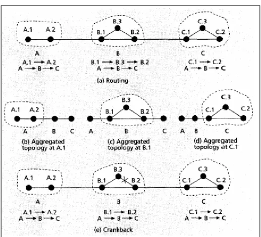
(20) distributed heuristics for the NP-complete routing problems, especially in the case of multicast routing, because there is no detailed topology and link-state information available. In addition, when the global states at different nodes are inconsistent, loops may occur. A loop can easily be detected when the routing message is received by a node for the second time. However, loops generally make the routing fail because vectors do not provide sufficient information for an alternative path.. 2.3.. Hierarchical Routing Algorithms. PNNI [24]-PNNI is a hierarchical link-state routing protocol [2]. Its hierarchical model was discussed earlier. We use an example to illustrate the routing process. The network in Fig.1a has a two-level hierarchy with three groups. The aggregated topology maintained at A.1, B.1 and C.1 are shown in Fig.1b, c, and d, respectively. Suppose every link has an available bandwidth of one. Consider a connection request arriving at A.1 with destination C.2. Let the bandwidth requirement be one. The routing process is described as follows. Based on the aggregated state, the source node A.1 finds a path (A.1->A.2) within its group and a logical path (A->B->C) on the higher hierarchy level. The logical path, together with the destination C.2 is sent to the next group B on the path. When the boarder node B.1 receives the information, it selects a path (B.1->B.2->B.3) within its group and then passes the logical path and the destination to group C. Finally, the boarder node C.1 of the destination group. 20.

(21) completes the routing by selecting C.1->C.2. It may happen that a link on the selected path does not have sufficient resources. Fig.1e gives an example, where link B.3->B.2 does not have enough bandwidth for the connection due to traffic dynamics. In this case, the routing process is cranked back to B.1 and resumes with an alternative path B.1->B.2.. Figure 1 An example of PNNI routing. 21.

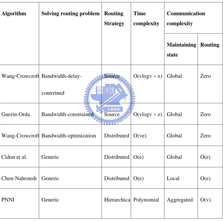
(22) 2.4.. Previous Work Summary. We classify those algorithms according the solving routing problem, routing strategy, time complexity, communication complexity. The details are listed in table 1.. Algorithm. Solving routing problem Routing Strategy. Time. Communication. complexity. complexity. Maintaining Routing state. Wang-Crowcroft Bandwidth-delay-. Source. O(vlogv + e) Global. Zero. Source. O(vlogv + e) Global. Zero. contrrined. Guerin-Orda. Bandwidth-constrained. Wang-Crowcroft Bandwidth-optimization. Distributed O(ve). Global. Zero. Cidon et al.. Generic. Distributed O(e). Global. O(e). Chen-Nahrstedt Generic. Distributed O(e). Local. O(e). PNNI. Hierarchical Polynomial. Aggregated. O(v). Generic. Table 1 Unicast routing algorithms. 22.

(23) 3.. Problem Model and Formulation In this chapter, we will describe our problem, and model it. Besides these, we also. formulate our problem into non-linear integer programming form. In the next two chapters, we will propose an algorithm based on Lagrangean Relaxation to solve this problem.. 3.1.. Problem Description. We construct the network into load balance model subject to end-to-end packet delay constraints for each individual user. This model has two advantages.. 1. This model can reduce packets delay implicitly.. 2. This model reserves the maximum flexibility to the later connections.. The problem has also been shown to be NP-complete which means no polynomial time algorithm for it unless P=NP. For the sake of obtaining sub-optimal solutions, Lagrangean relaxation is applied to the formulation to decompose the problem into several tractable subproblems in next chapter. The candidate path set does not need to be prepared in advance and the best paths are generated while solving the subproblems in our approach. A heuristic algorithm based on the solving procedure of the Lagrangean relaxation will be developed to obtain a primal feasible solution in the next two chapters.. 23.

(24) 3.2.. Network Model and Definition. A virtual circuit communications network is modeled as a graph where the processors are represented by nodes and the communication channels are represented by arcs. Let. V = {1, 2, 3, ..........., N} be the set of nodes in the graph and let L denote the set of communication links in the network. Let W be the set of origin-destination (O-D) pairs (commodities) in the network. For each O-D pair w ∈ W , the arrival of new traffic is modeled as a Poisson process with rate rw (packet/sec). To reduce the problem’s complexity, we assume that each O-D pair w, the overall traffic is transmitted over one path in the set Pw . For each link l ∈ L , the capacity is Cl packets/sec.. For each O-D pair w ∈ W , let x p be 1 when p ∈ Pw is used to transmit packets for O-D pair w and 0 otherwise. In a virtual circuit network, all of the packets in a session are transmitted over exactly one path from the origin to the destination. Thus. ∑x. p∈Pw. p. = 1 . For each. path p and link l ∈ L , let δ pl denote the indicator function which is 1 if link l is on path p and 0 otherwise. Then, the aggregate flow over link l, denote as gl , is. ∑ ∑x rδ. p∈Pw w∈W. p w. pl. .. In the network, there is a buffer for each outbound link. Using Kleinrock’s independence assumption [16], the arrival of packets to each buffer is a Poisson process where the rate is the aggregate flow over the outbound link. It is assumed that the transmission time for each −1. packet is exponential distributed with mean Cl . Thus, each buffer is modeled as an M/M/1. 24.

(25) queue, as considered in [1, 8, 4].. 3.3.. Problem Formulation. An non-linear integer formulation is developed to formulate the QoS routing problem for load balancing purpose. The constraints are required to satisfy the traffic demand constraint, QoS required constraint and physical capacity limitations. The outputs are the routing path for each O-D pair. The following notations are used in the formulation.. Input values:. N F : the set of nodes in the network.. L. : the set of communication links in the communication network.. W. : the set of source-destination (SD) pairs.. Wn : the set of SD pairs where node n is the source node. rw :(packets/sec.):the arrival rate of new traffic of each O-D pair w ∈W ,which is. modeled of Poisson process for illustration purpose. Cl. : (packets/sec.),the capacity of each link l ∈ L .. Pw : a given set of of simple directed paths from the origin to the. destination of O-D pair w ∈W . gl. : the aggregate flow over link l, which is equal to. ∑ ∑x rδ. p∈Pw w∈W. p w. pl. .. δpl : 1 if path p uses link l; 0 otherwise. 25.

(26) Dw : the maximum allowable end to end delay for O-D pair w ∈W .. Decision variables:. α. :percentage of capacity usage on maximum congested link.. xp. : 1 if path p is selected, 0 otherwise. The formulation is modeled as the following integer linear programming problem.. Problem P min α. Subject to: gl =. ∑ ∑x rδ p w. p∈Pw w∈W. pl. x pδ pl. ∑∑C l∈L p∈Pw. l. − gl. ∑x. p∈Pw. p. xp. ≤ α Cl. ∀l ∈ L. (1). ≤. Dw. ∀w ∈ W. (2). =. 1. ∀w ∈ W. (3). ∀p ∈ Pw , w ∈ W. (4). = 0 or 1. 0 ≤α ≤1. (5). The objective function is to minimize the largest utilization on the most congested link. Constraint (1) requires the capacity used on every link must less than the one on the most. 26.

(27) congested link. Constraint (2) requires the end-to-end delay should be no large than Dw for each O-D pair. Constraint (3) is the routing constraint. It also requires all traffic demands must be satisfied. Path selection or not is expressed as a binary variable in Constraint (4). The utilization is a real number between zero and one, which is described in Constraint (5). For the purpose of applying Lagrangean relaxation method, we transform the above problem formulation into an equivalent formulation PII. In PII, two auxiliary variables are introduced: ywl is defined as. ∑xδ. p∈Pw. p. pl. and fl denotes the estimate of the aggregate. flow.. Decision variables: α. :percentage of capacity usage on maximum congested link.. xp. : 1 if path p is selected, 0 otherwise.. ywl : 1 if source-destination pair w uses link l, 0 otherwise.. 27.

(28) Problem PII. min α. Subject to: fl ≤ α Cl ywl l − fl. ∑C l∈L. ∑xδ. p∈Pw. p. ≤. Dw. ≤. pl. ywl. gl ≤ fl. ∑x. p∈Pw. p. =. 1. ∀l ∈ L. (1). ∀w ∈ W. (2). ∀w ∈ W , l ∈ L. (3). ∀l ∈ L. (4). ∀w ∈ W. (5). xp. = 0 or 1. ∀p ∈ Pw , w ∈ W. (6). ywl. = 0 or 1. ∀w ∈ W , l ∈ L. (7). 0 ≤α ≤1 0 ≤ fl ≤ Cl. (8) ∀l ∈ L. (9). Redundant constraints associated with these auxiliary variables (3) ,(4),(7) and (9) are added. It is clear that the equality should hold at the optimal point. By introducing these auxiliary variables, the Lagrangean relaxation problem can be decomposed into independent and easily solvable subproblems. In network optimization problem, it can usually be found that the desired problem consists of several special embedded structures which might have been well studied and 28.

(29) exist well-known algorithms to optimally solve them efficiently. However, the original problem may be a very difficult one due to its ill mathematical structures, large problem size, or complex integer/combinatorial property; even if we can solely handle all of its embedded modules efficiently. Another kind of problems is NP-complete/NP-hard problems. Since these problems cannot be modeled as polynomial time solvable programs unless P=NP, efficient heuristic algorithm or approximation algorithm has to be developed for these problems. Especially, when the problem size of the desired problem is out of the computation power by using exhaustive search or other exact evaluation methods. In order to deal with these intractable features, one might try to get near optimal solutions instead of casting the real optimal solutions. Thus, performing some relaxation to the design problem is necessary in solving these problems. Lagrangian relaxation is a general solution strategy for solving mathematical programs that permits us to decompose original problems into several subproblems such that we can exploit their special embedded structures. Lagrangean relaxation can provide bound on the value of the optimal objective function and the bound outperform those provided by linear programming relaxation in many instances [20]. Furthermore, the solutions of Lagrangean relaxation problem provide a good base to help designer to develop effective heuristic algorithms for the desired problems.. 29.

(30) In the next chapter, we use Lagrangean relaxation to the heterogeneous Minmax end to end delay problem and decompose the original problem into several subproblems.. 30.

(31) 4.. Lagrangean relaxation and problem decomposition. We first dualize Constraints (1), (2), (3) and (4) to Problem PII to obtain the following Lagrangean relaxation problem.. Problem (Dual_P): Z dual ( ρ ) = min{[1 − ∑ vl cl ]α + [ ∑ sw (∑ l∈L. w∈W. ∑ ∑t ( ∑ x δ. w∈W l∈L. wl. p∈Pw. p. pl. l∈L. ywl − Dw )] + cl − fl. − ywl ) + ∑ [ul ( gl − fl ) + vl f l ]} − (∗) l∈L. subject to constraints (5), (6), (7), (8), and (9) .. ∑x. p∈Pw. =. p. 1. ∀w ∈ W. (5). xp. = 0 or 1. ∀p ∈ Pw , w ∈ W. (6). ywl. = 0 or 1. ∀w ∈ W , l ∈ L. (7). 0 ≤α ≤1. (8). 0 ≤ fl ≤ Cl. ∀l ∈ L. (9). Reorganizes formulation (*), dual (P) becomes => Z dual ( ρ )= min{[1 − ∑ vl cl ]α + [ ∑ ∑ ∑ (twl + ul rw ) x pδ pl ] l∈L. +[∑ ( l∈L. ∑s. w∈W. w. ywl. cl − fl. w∈W l∈L p∈Pw. − ∑ twl ywl + (vl −ul ) f l ) − ∑ sw Dw ]} w∈W. w∈W. subject to Constraints (5), (6), (7), (8), and (9) 31.

(32) and vectorρ= (s,t,u,v) is the non-negative Lagrangean multiplier.. Problem (Dual_P) can be decomposed into following three independent subproblems. (S1, S2 and S3) by separating the decision variables α, x, y. Therefore, we have Zdual=ZS1+ ZS2 +ZS3 −. ∑s. w∈W. w. Dw , where.   ZS1(v)= min 1 − ∑ vl cl α  l∈L  subject to Constraint (8),. ZS2(t,u)= min [. ∑ ∑ ∑ (t. w∈W l∈L p∈Pw. wl. + ul rw ) x pδ pl ]. subject to Constraints (5) and (6) , and. ZS3(s,t,u,v)= min{∑ ( l∈L. ∑s. w∈W. w. ywl. cl − fl. − ∑ twl ywl + (vl −ul ) fl )} w∈W. subject to Constraints (7) and (9). We will solve these three subproblems using linear algorithms in next three sections.. 32.

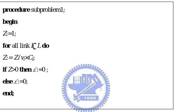
(33) 4.1.. Solving Subproblem 1. Subproblem S1 is a problem for decision variable α. Variableαis set to 1 if the corresponding cost 1 − ∑ vl cl is negative; otherwiseαis set to 0. Subproblem 1 runs on l∈L. O(L) computation time.. procedure subproblem1; begin Z:=1; for all link l∈L do Z:= Z−vl×Cl; if Z>0 then α:=0 ; else α:=0; end;. Figure 2 The algorithm of Subproblem 1. 33.

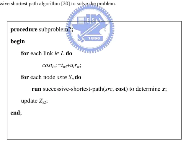
(34) 4.2.. Solving Subproblem 2. Subproblem S2 is a problem for decision variable x. It consists of |Wn| (one for each source node) independent problems. Each one is an edge-disjoint-path problem rooted at the given source node and destined to all destination nodes for the SD pairs with non-zero traffic demand. To solve the problem, one can view the input network as a graph. This graph contains (L) arcs and (N) nodes. We set each arc l have Cl capacity (it means that the transmission time for each packet is exponentially distributed with mean Cl) and non-negative arc weight, (twl+ulrw) . In such graph, the subproblem is a minimum cost flow problem to send minimum cost flow from the source node to all its destination nodes with specified traffic demands. We use traditional minimum cost flow algorithm such as successive shortest path algorithm [20] to solve the problem.. procedure subproblem2; begin for each link l∈L do costlw:=twl+ulrw; for each node src∈Sn do run successive-shortest-path(src, cost) to determine x;. update Zs2; end;. Figure 3 The algorithm of Subproblem 2. 34.

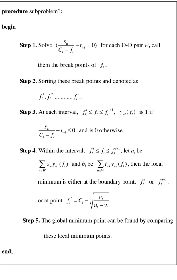
(35) 4.3.. Solving Subproblem 3. Subproblem S3 is a problem for decision variable y. It consists of |L| (one for each link l ∈ L ) independent problems.. For each link l ∈ L :. ∑s. min[. w∈W. w. ywl. cl − f l. − ∑ twl ywl + (vl − ul ) fl ] w∈W. subject to (5) and (8).. For different values of fl, the value of ywl for minimum objective function, denoted as *. ywl ( f l ) may be different. As an example, consider the case that fl =0. The objective *. function is minimized by assigned ywl (0) to 1 if (. sw − twl ) ≤ 0 and to 0 otherwise. We cl. define a set of break points of fl as those points where ( 1. sw − twl ) = 0 for each w. These Cl − fl n. 2. break points are sorted and denoted as fl , f l ,.............. f l . Note that there are at most |W| break points. We observe that when fl ≤ fl ≤ fl i. i +1. *. the value, the value of ywl ( f l ). remains constant for all w ∈ W . Within the above internal, ywl ( f l ) is 1 if *. (. sw i i +1 − twl ) ≤ 0 and is 0 otherwise. Therefore, within an interval, [ fl , fl ) , the cl − f l. objective is only a function of fl, and the minimum point within the interval can be found analytically. By examining at most |W| +1 intervals, we can find the global minimum point by comparing those local minimum points. *. i. When examining an interval, we first determine ywl ( f l ) within the interval for. 35.

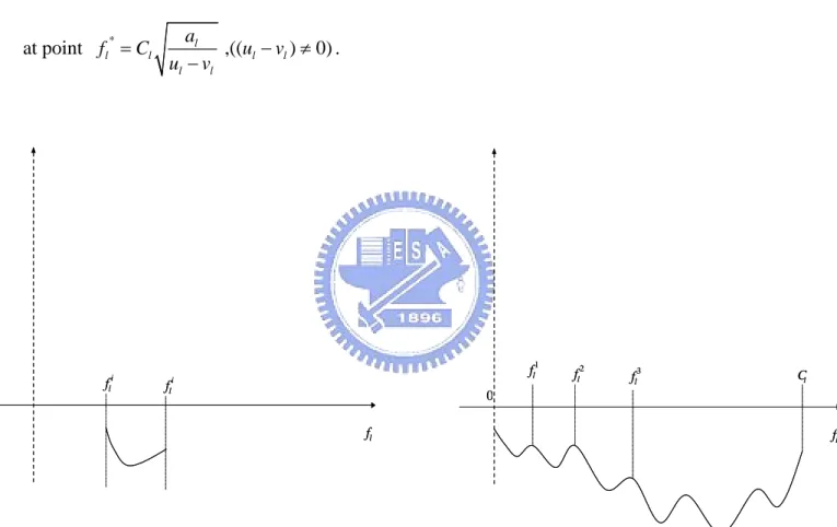
(36) ∑s. each w. We denote. w∈W. *. w. i. ywl ( fl ) as al and. ∑t. w∈W. *. wl. i. ywl ( f l ) as bl. Note that al and bl are. non-negative. Within the interval, the objective function can then be expressed as:. Z sub 3_ l =. al − bl + (vl − ul ) fl . A typical curve of the objective function vs. fl within the Cl − f l. interval fl ≤ fl ≤ fl i. i +1. is shown in Figue 1. The curve of the objective function vs. fl is i. shown in Fig. 2. The local minimum point is either at the boundary point, fl or fl at point fl = Cl *. fli. i +1. , or. al ,((ul − vl ) ≠ 0) . ul − vl. fl1. fli. fl2. fl3. Cl. 0. fl. Figure 4 A typical curve of the objective function of (SUB3) vs. fl. fl. Figure 5 A typical graph of the objective function of (SUB3) vs. fl. 36.

(37) procedure subproblem3; begin Step 1. Solve (. sw − twl = 0) for each O-D pair w, call Cl − fl. them the break points of fl . Step 2. Sorting these break points and denoted as 1. 2. n. f l , fl ............, f l . i +1. Step 3. At each interval, f l ≤ fl ≤ fl , ywl ( f l ) is 1 if i. sw − twl ≤ 0 and is 0 otherwise. Cl − fl i +1. Step 4. Within the interval, fl ≤ f l ≤ f l , let al be i. ∑s. w∈W. w. ywl ( f l ) and bl be. ∑t. w∈W. wl. ywl ( f l ) , then the local i. i +1. minimum is either at the boundary point, fl or f l , or at point f l = Cl − *. al . ul − vl. Step 5. The global minimum point can be found by comparing. these local minimum points. end;. Figure 5 The algorithm of Subproblem 3. 37.

(38) 4.4.. Subgradient Optimization Procedure. From the weak Lagrangian duality theorem, Zdual(ρ) is a lower bound of the Problem (P) for any non-negative Lagrangean multiplier vector ρ = (s, t, u ,v) ≥ 0. Naturally, one wants to determine the largest lower bound by Zlower_bound = max Z dual ( ρ ) ρ ≥0. (11). The subgradient method can be applied to solve (11). The solution to Problem (Dual_P) at iteration k of the subgradient optimization procedure is given below. In subgradient solution procedure, the Lagrangian multiplier vector ρ is updated by. ρ k +1 = ρ k + θ k bk. where b is a subgradient of Zdual(ρ) with vector size |W+LW+L+L|. The step size θ k is determined by. θk =. λk (UB − Z dual ( ρ )) bk. 2. UB is an upper bound obtained from a heuristic solution described in the next section and. λk is a constant in a range from 0 to 2. The details of this procedure see below:. 38.

(39) procedure update-step-size; begin y wl − Dw ; l∈L C l − f l. ∀ bi:= ∑. 1≤ i≤| w|. ∀. | W|+1≤i ≤|W |+| L||W |. ∀. bi:= ∑ x pδ pl − y wl ; p∈ p w. |W |+| L||W |+1≤ i ≤|W |+| L||W |+| L|. bi:= g l − f l ;. ∀. |W |+| L||W |+1≤ i ≤|W |+| L||W |+| L|+| L|. bi:= f l − αCl ;. step size θ = λ (UB − Z dual ) / b ; 2. end; procedure update-multiplier; begin for l:=1 to |W| do y wl + − Dw )] ; l∈L C l − f l. sw:=[sw+θ ( ∑ for l:=1 to |L| do. for w:=1 to |W| do. tlw:= [tlw+θ (. ∑x δ. p∈ p w. p. +. pl. − y wl )] ;. for l:=1 to |L| do. ul:= [ul+θ ( g l − f l )]+ ; for l:=1 to |L| do. vl:= [vl+θ ( f l − αCl )]+ ; end;. Figure 6 The algorithm of update-step-size and update-multiplier 39.

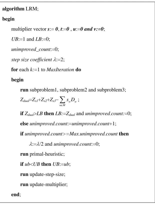
(40) 4.5.. Summary of Lagrangean Relaxation Method. The algorithms are described below: LRM denotes the Lagrangean relaxation method.. algorithm LRM; begin. multiplier vector s:= 0, t:=0 , u:=0 and v:=0; UB:=1 and LB:=0; unimproved_count:=0; step size coefficient λ:=2; for each k:=1 to MaxIteration do begin run subproblem1, subproblem2 and subproblem3;. Zdual=Zs1+Zs2+Zs3− ∑ sw Dw ; w∈W. if Zdual>LB then LB:=Zdual and unimproved-count:=0; else unimproved-count:=unimproved-count+1; if unimproved-count>=Max-unimproved-count then. λ:=λ/2 and unimproved-count:=0; run primal-heuristic; if ub<UB then UB:=ub; run update-step-size; run update-multiplier; end;. Figure 7 The algorithm of LRM. 40.

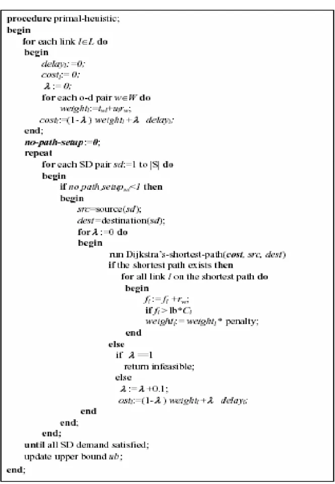
(41) 5.. Lagrangean-based Heuristic Algorithm. Since the Lagrangean relaxation is obtained by the relaxation of some constraints from the problem formulation, the solution to the dual problem might be infeasible for the original primal problem resulting from dissatisfaction of those relaxed constraints. However, such solution can still be used as a base to develop efficient heuristic algorithms to seek feasible solutions and obtain upper bounds for the original problem. In practice, at each iteration of the subgradient solving procedure, the solution of Lagrangean relaxation is used to obtain a lower bound of the primal problem. In addition, we verify the feasibility of the solution in the constraints of primal problem. If the solution is feasible, it is used to calculate an upper bound of the primal problem (Actually it is an optimal solution.). If the solution is not feasible, the following heuristic is applied to find a feasible solution.. 5.1.. Proposed Lagrangean-based Heuristic Algorithm. Based on the solution obtained from solving Lagrangean relaxation in each iteration. We observe that when solving xp in subproblem 2, we set the cost of each link be (twl + ulrw), so if we take the same paths in LRM, the gap between LB and UB will be minimum. But not all of these paths can be selected (due to some constraints are violated), so the cost of each. Costl = (1- λ )Weightl + λ Delayl ; initial λ = 0 .. link is modify to . Traffic demands are then routed onto the network for each SD pair sequentially (from short delay required connections to long delay required ones) by applying Dijkstra’s shortest path algorithm. The capacity of those arcs used by the above accepted paths are updated by subtracting the flow of this connection from the capacity of this link. If the utilization of a link will become greater than the best known lower bound (LB)×|Cl| when a 41.

(42) further virtual circuit setups on it, the weight of this arc is replaced by multiply a constant term on its weight as a penalty for avoiding further setup paths on this link. The process continues until all of the traffic demands are satisfied or the network cannot accommodate the traffic request. A feasible solution is obtained in the former case.. 5.2.. Evaluation of the Feasible Schedule. From the weak Lagrangian duality theorem, Zdual(ρ) is a lower bound of the Problem (P) for any non-negative Lagrangean multiplier vector ρ = (s, t, u ,v) ≥ 0. Naturally, one wants to determine the largest lower bound by Zlower_bound = max Z dual ( ρ ) ρ ≥0. (11). The subgradient method can be applied to solve (11). The entire procedure is described below.. Initialization. solving Subproblem_1. Subproblem_. Subproblem_ Subgradient method to update multipliers. Obtain feasible routing scheme by heuristic. Compute Duality Gap. Result good enough ?. No. Yes Stop. Figure 8 The algorithm of LRM Evaluation Procedure 42.

(43) Figure 9 The algorithm of Primal-Heuristic. 43.

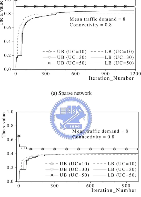
(44) 6. Experimental Results We have carried out a performance study on LRH and drawn a comparison between LRH and the LPH approach via experiments over randomly generated networks. Given the total number of nodes, say n, the greatest possible number of bi-directional links is C2n , where C is the combination operation. Then, for a network with n nodes and a connectivity, t, it is generated by randomly selecting C (n, 2) × t out of the C (n, 2) bi-directional links of the network.. 6.1.. Performance Study. We carried out two sets of experiments over 15-node random networks with two connectivities v=0.4 and 0.8, which correspond to sparse and dense networks, respectively. In the first set of set of experiments, the LRH algorithm was terminated when the number of iteration exceeded a pre-determined Iteration_Number, ranging from 0 to 1500. Numerical results are displayed in Figure 12. We study both the lower and upper bounds on α under different UC values. We observe that while the upper bound performance is irrelevant to UC, the lower bound performance is highly dependent on the UC setting in the same manner as above. Specifically, smaller UC values yield faster convergence but only to looser lower bounds, while larger UC values result in tighter lower bounds through gradual convergence over a larger number of iterations. This fact reveals that, by adjusting the UC value, the LRH approach is capable of balancing the trade-off between accuracy and efficiency for resolving various types of our problems.. 44.

(45) The α value. 1 .0 0 .8 M ean traffic d e m an d = 8 C o n n ectiv ity = 0 .8. 0 .6 0 .4. U B (U C = 1 0 ) U B (U C = 3 0 ) U B (U C = 5 0 ). 0 .2. L B (U C = 1 0 ) L B (U C = 3 0 ) L B (U C = 5 0 ). 0 .0. 0. 300. 600. 900. 1200. Iteratio n _ N u m b er. The α value. (a) Sparse network. 1 .0 0 .8 M ean traffic d e m an d = 8 C o n n ectiv ity = 0 .8. 0 .6 0 .4. U B (U C = 1 0 ) U B (U C = 3 0 ) U B (U C = 5 0 ). 0 .2. L B (U C = 1 0 ) L B (U C = 3 0 ) L B (U C = 5 0 ). 0 .0. 0. 300. 600. 900. Iteratio n _ N u m b er. (b) Dense network Figure 10 Convergence speed versus accuracy on the basis of using fixed iteration number.. 45.

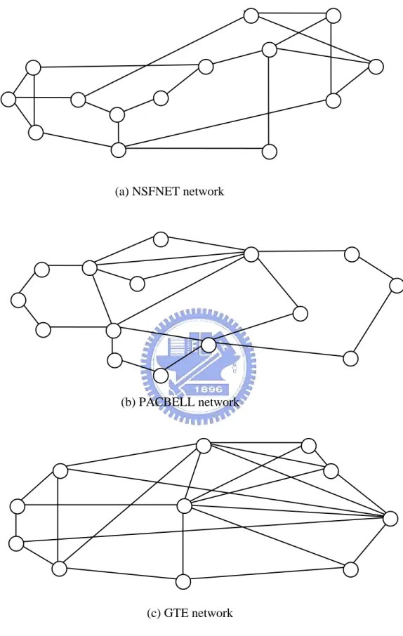
(46) 6.2.. Performance Comparisons. We first carried out numerical computation of the lower and upper bound values of α , the maximum aggregate arrival rates of a link divided by the capacity of each link, Cl , using our LRM-based method and a Linear Programming Relaxation (LPR)-based method. In the computation, we considered three widely used networks. They are: NSFNET with 14 nodes and 42 links; PACBELL with 15 nodes and 42 links; and GTE with 11 nodes and 46 links. In the LRM-based heuristic algorithm, we adopted a penalty term of 2. In addition, if the Lagrangean lower bound remains unimproved for 50 iterations (UC=50), the step size coefficient (λk ) would be divided by two. The simulation was written in the C language and terminated at the end of 2000 iterations and operated on a PC running Windows XP with a 1.8 GHz CPU power.. In the LPR-based method, by removing Constraints (6) and (7), the original Integer Linear Programming (ILP) problem is relaxed to a Linear Programming (LP) problem. Thus, the solution to the relaxed problem is a legitimate lower bound of the original ILP problem. To obtain an upper bound, we also develop a corresponding heuristic algorithm. The algorithm ranks all SD pairs in accordance with the desired packet delay. The next feasible path founded in the LP solution is then assigned to the SD pair with the smallest packet delay. There may be multiple feasible paths for an SD pair; we select the shortest path with the largest xp value in the algorithm. The path assignment process repeats until either the traffic demands of all SD pairs are satisfied (i.e., feasible), or there is no remaining resource (i.e., infeasible). In the simulation, the LP problem was solved using the CPLEX software, operating in the same PC environment previously described.. 46.

(47) Numerical results for the NSFNET, PACBELL, and GTE are summarized in Table II, III, and IV, respectively. The traffic demands (i.e., the traffic arrival rate) for all SD pairs are randomly determined with their mean value shown in the first column of the tables. Moreover, the Gap in the third column of the tables is computed as the ratio of the difference of the upper and lower bounds to the lower bound in percentage. As shown in Table II for NSFNET, the LPR-based method reaches a low guarantee of 20% gap, incurring high CPU computation time. Compared to it, the LRM-based method achieves ideal lower and upper bounds (gap< 5%) under all four traffic demand cases except case 1. The algorithm also improves the CPU computation time by one order of magnitude. We discover that, even though both methods achieve optimal lower bounds, the LRM-based heuristic algorithm arrives at much improved upper bounds due to the use of the Lagrangean multipliers derived upon seeking the Lagrangean relaxation solution. In Table III for PACBELL, the LPR-based method reaches a low guarantee of 29% gap. Compared to it, the LRM-based method again achieves ideal lower and upper bounds (<8%). The LRM-based algorithm also improves the CPU computation time by two order of magnitude. It is worth mentioning that in the case of the mean traffic demand being equal to 3.0, while the LPR-based method fails to obtain a feasible solution, the LRM-based method arrives at the optimal solution. Finally, in Table IV for the GTE network, the LRM-based method outperforms the LPR-based method in both the solution superiority and the computation time in all traffic cases. Specifically, the LPR-based method again reaches fairly low guarantee of 27% gap. The method produces a non-optimal solution but with an improved guarantee of 13% gap. This justifies the viability of the LRM-based method for providing efficient QoS routing method. 47.

(48) (a) NSFNET network. (b) PACBELL network. (c) GTE network. Figure 11 Three networks. 48.

(49) Table 2 Numerical results for NSFNET Network Demand. LB. LP_UB. LP Lag_CPU Lag_Diff LP_CPU LP_Diff Lag Lag_UB % Feasibility (sec) (sec) % Feasibility. 5. 0.134885 0.15625. 1108. 15.840. Yes. 0.156250. 28. 15.840. Yes. 10. 0.260588 0.31250. 1694. 19.921. Yes. 0.281250. 41. 7.929. Yes. 15. 0.403905 0.46875. 1754. 16.055. Yes. 0.406250. 54. 0.581. Yes. 20. 0.533426 0.62500. 1809. 17.167. Yes. 0.562500. 64. 5.450. Yes. 25. 0.646050 0.75000. 1947. 17.152. Yes. 0.656250. 71. 1.579. Yes. 30. 0.820311 0.90625. 2027. 10.476. Yes. 0.843750. 82. 2.857. Yes. Table 3 Numerical results for PACBELL Network Demand. LB. LP Lag_CPU Lag_Diff LP_CPU LP_Diff Lag Lag_UB % Feasibility (sec) (sec) % Feasibility. LP_UB. 10. 0.289678 0.375000. 2335. 29.454. Yes. 0.312500. 41. 7.878. Yes. 15. 0.448961 0.531250. 2151. 18.329. Yes. 0.468750. 53. 4.408. Yes. 20. 0.596959 0.687500. 2414. 15.167. Yes. 0.625000. 67. 4.697. Yes. 25. 0.757723 0.906250. 2697. 19.602. Yes. 0.781250. 80. 3.105. Yes. 30. 0.951497. 2651. NA. No. 0.96875. 90. 1.812. Yes. NA. Table 4 Numerical results for GTE Network Demand. LB. LP_UB. LP Lag_CPU Lag_Diff LP_CPU LP_Diff Lag Lag_UB % Feasibility (sec) (sec) % Feasibility. 10. 0.177474 0.218750. 410. 23.257. Yes. 0.187500. 65. 5.649. Yes. 15. 0.270522 0.343750. 440. 27.069. Yes. 0.281250. 85. 3.966. Yes. 20. 0.348616 0.406250. 712. 16.532. Yes. 0.375000. 103. 7.568. Yes. 25. 0.406115 0.468750. 830. 15.423. Yes. 0.437500. 124. 7.728. Yes. 30. 0.468669 0.562500. 897. 20.020. Yes. 0.531250. 135. 13.353. Yes. 35. 0.546826 0.687500. 912. 25.726. Yes. 0.593750. 148. 8.581. Yes. 40. 0.616869 0.687500. 954. 11.450. Yes. 0.656250. 157. 6.384. Yes. 45. 0.655807 0.750000. 1024. 14.363. Yes. 0.718750. 160. 9.598. Yes. 50. 0.701118 0.781250. 1231. 11.429. Yes. 0.75000. 162. 6.972. Yes. 55. 0.804162 0.906250. 1403. 12.695. Yes. 0.875000. 174. 8.809. Yes. 49.

(50) We further draw comparisons of accuracy and computation time between our LRH approach and the Linear Programming Relaxation (LPR)-based method. For generating networks, it is impractical to experiment on networks with smaller numbers of nodes and links. However, for networks with greater than 12 nodes, we experienced that the computation time using the LPR-based method became unmanageable. In the experiment, we considered three random networks, called NET1, NET2, and NET3, as shown in Figure 13. NET1 consists of 10 nodes, and 19 bi-directional links, corresponding to a connectivity (v) of 0.44 . NET2 consists of 11 nodes, and 22 bi-directional links, corresponding to a connectivity (v) of 0.4. NET3 consists of 11 nodes, and 22 bi-directional links, corresponding to a connectivity (v) of 0.4. Numerical results are demonstrated in Figures 14. In the computation using our LRH approach, we adopted UC=50 and two different termination criteria. The two criteria are: Iteration_Number=1000, and 2000. The algorithm was written in the C language and operated on a PC running Windows XP with a 1.8GHz CPU power. In the LPR-based method, by removing Constraints (6) and (7), the original Integer Linear Programming (ILP) problem is relaxed to a Linear Programming (LP) problem. Thus, the solution to the relaxed problem is a legitimate lower bound of the original ILP problem. The upper bound is then obtained according to the randomization procedure proposed in previous. In the experiment, the LP problem was solved using the CPLEX software, operating in the same PC environment. For both approaches, the accuracy is measured in terms of the Gap(%) which is defined as the ratio of the difference of the UB and LB of α to the LB value in percentage. As shown in the three figures, the LPR-based method exhibits larger gaps, namely poorer accuracy, and requires high computation time under both networks. In contrast, the. 50.

(51) LRH-based method achieves ideal lower and upper bounds under several traffic demand cases. In fact, we discover that, both LRH and LPR-based approaches achieve tight lower bounds. Significantly, the LRH heuristic algorithm arrives at much improved upper bounds due to the use of the Lagrangean multipliers derived upon seeking the Lagrangean relaxation solution. Specifically, we discover from Figure 14 that the LRH approach using the 1000 iterations achieves as high accuracy as that using the 2000 iterations criterion under most demand cases.. Furthermore, as shown in Figure 15, the LRH approach outperforms the LPR-based method in computation time by at least one order of magnitude under all cases. Notice that, the LRH approach using the fixed iteration =1000 incurs exceptionally low computation, and achieves as high accuracy as that using the 2000 iterations criterion under most demand cases. Compared to the LPR-based method, the LRH approach offers an improvement of computation time by more than two orders of magnitude.. 51.

(52) (a) NET1 (10 nodes). (b) NET2 (11 nodes). (c) NET3 (11 nodes). Figure 12 Three random generating networks.. 52.

(53) LRH(Iteration_Number=1000) LRH(Iteration_Number=2000) LPH. 40. Gap (%). Gap (%). 50. LRH(Iteration_Number=1000) LRH(Iteration_Number=2000) LPH. 60 50 40. 30. Node number = 10 Connectivity = 0.44. Node number =11 Connectivity =0.4. 30. 20. 20 10. 10 0. 0. 10. 15. 20 25 30 Mean traffic arrival rate. Gap (%). (a) NET1. 5. 10. 15. 20 25 30 Mean traffic arrival rate (b) NET2. 50 LRH(Iteration_Number=1000) LRH(Iteration_Number=2000) LPH. 40. Node number = 11 Connectivity = 0.4. 30 20 10 0. 0. 10. 20. 30. 40 50 60 70 Mean traffic arrival rate. (c) NET3. Figure 13 Comparison of accuracy under three random networks.. 53.

(54) Computation Time (sec). Computation Time (sec). LPH LRH(2000) LRH(1000). 2000 1500 1000 500 0. 5. 10. 15. 20. 25. Mean Traffic Demand. (a) NET1. Computation Time (sec). 500 400 300 200 100 0. 30. LPH LRH(2000) LRH(1000). 0. 5. 10. 15. 20. 25. 30. (b) NET2. LPH LRH(2000) LRH(1000). 2000. 1500. 1000. 500. 0. 5. 15. 25. 35. 45. 35. Mean Traffic Demand. 55. Mean Traffic Demand. (c) NET3. Figure 14 Comparison of computation time under three random networks.. 54.

(55) 7.. Conclusions and Future Works In this thesis, we have improved a QoS routing problem using a Lagrangean Relaxation. based approach augmented with an efficient primal Heuristic algorithm, called LRH. With the aid of generated Lagrangean multipliers and lower bound indexes, the primal heuristic algorithm of LRH achieves a near-optimal upper-bound solution. In our thesis, we have three major characteristics which are compared with other proposed methods. First, we start to consider user’s perspective and system’s perspective jointly. Second, in our routing procedure, the candidate path set does not need to be prepared in advance and the best paths are generated while solving the subproblems in our approach. Third, our method can both provide the upper bound and lower bound to the problem, this distinguishing feature can help us to verify the performance of our solutions. A performance study delineated that the performance trade-off between accuracy and convergence speed can be manipulated via adjusting the Unimproved Count (UC) parameter in the algorithm. We have drawn comparisons of accuracy and computation time between LRH and the Linear Programming Relaxation (LPR)-based method, under three networks NSFNET, PACBELL, and GTE and three random networks. Experimental results demonstrated that the LRH is superior to the other approach, namely the LPR method in both accuracy and computational time complexity, particularly for larger size networks.. 7.1.. Future Works. A future work we can do is that we are able to reconfigure the virtual topology to adapt to changing traffic patterns. Some reconfiguration studies on virtual networks have been reported before [7, 12, 9]; however, these studies assumed that the new virtual topology was. 55.

(56) known a priori, and were concerned with the cost and sequence of branch-exchange operations to transform from the original virtual topology to the new virtual topology. We propose a methodology to obtain the new virtual topology, based on optimizing a given objective function, as well as minimizing the changes required to obtain the new virtual topology from the current virtual topology. This approach would result in the minimum number of switch re-tunings, thus minimizing the number of disrupted virtual paths. Consequently, this approach also minimizes the time it takes to complete the reconfiguration process. Some discussions on the control mechanisms required to perform re-tunings of virtual paths can be found in [21].. In the ideal situation, given a small change in the traffic matrix, we would prefer for the new virtual topology to be largely similar to the previous virtual topology, in terms of the constituent virtual paths and the routes for these virtual paths, i.e., we would prefer to minimize the changes needed to adapt from the existing virtual topology to the new topology. More formally, it would be preferable if a large number of the δ pl variables retain the same values in the two solutions, without compromising the quality of the solution (in terms of minimizing the congested link utilization).. Let us consider the snapshot of two traffic matrices, λsd1 and λsd2 , taken at two not-too-distant time instants. We assume that there is a certain amount of correlation between. 56.

(57) these two traffic matrices. Given a certain traffic, there may be many different virtual topologies, each of which has the same optimal value with regard to the objective function. But we will terminate after the first such optimal optimal solution is found. Our reconfiguration algorithm finds the virtual topology corresponding to λsd2 which matches “closest” with the virtual topology corresponding to λsd1 (based on our above definition of “closeness”).. 7.2.. Reconfiguration Algorithm. We perform the following sequence of actions: 1). Generate formulations F (1) and F (2) corresponding to traffic matrices λsd1 and λsd2 , respectively, based on the formulation in Section 3.. 2). Derive solutions S (1) and S (2) , corresponding to F (1) and F (2) , respectively. Denote the variables’ values in S (1) as x p (1) and ywl (1) , and those in S (2) as x p (1) and ywl (1) , respectively. Let the value of the objective function for S (1) and. S (2) be OPT1 and OPT2 , respectively.. 3). Modify ( F (2) to F '(2) ) by adding the new constraint. α = OPT2. (10). This ensures that all the virtual topologies generated by F '(2) would be optimal with. 57.

(58) regard to the objective function.. The new objective function for F '(2) is Minimize: ∑∑ ywl (1) − ywl (2) w. (12). l. Note that the mod operation, x , is a nonlinear function. If we assume that ywl can only take. on. binary. values,. then. (12). become. linear,. i.e.,. if. ywl (1) = 1 ,. then. ywl (1) − ywl (2) ≡ (1 − ywl (2)) ; else if ywl (1) = 0 , then ywl (1) − ywl (2) ≡ ywl (2) . Hence, F '(2). may be solved directly.. 58.

(59) Reference [1] A. Shaikh, J. Rexford, and K. Shin, “Dynamics of quality-of-service routing with inaccurate link-state information”. U. of MI Tech. rep. CSE-TR-350-97, Nov. 1997. [2] ATM Forum, Private Network Network Interface (PNNI) v1.0 Specifications, May 1996. [3] B. Gavish and S.L. Hantler, “An Algorithm for Optimal Route Selection in SNA Networks”. IEEE Trans. on Communications COM-31, pp. 1154-1160, Oct. 1983. [4] B. Awerbuch et al., “Throughput- Competitive On-line Routing”. 34th Annual Symp.. Foundations of Comp. Sci., Pala Alto, CA, Nov. 1993. [5] B. Awerbuch et al., “Competitive Routing of Virtual Circuits with Unknown Duration”.. 5th ACM-SIAM Symp. Discrete Algorithms, Jan. 1994. [6] D. H. Lorenz and A. Orda, “QoS Routing in Networks with Uncertain Parameters”.. IEEE INFOCOM ’98, Mar. 1998. [7] D. Bienstock and O. Gunluk, “A degree sequence problem related to network design”. Networks, vol. 24, no. 4, pp. 195–205, July 1994. [8] F. Y. S. Lin and J. R. Yee, “A New Multiplier Adjustment Procedure for the Distributed Computation of Routing Assignments in Virtual Circuit Data Networks”. ORSA. Journal on Computing, Vol. 4, No. 3, Summer 1992. [9] G. N. Rouskas and M. H. Ammar, “Dynamic reconfiguration in multihop WDM. 59.

(60) networks”. J. High Speed Networks, vol. 4, no. 3, pp. 221–238, 1995. [10] H. F. Salama, D. S. Reeves, and Y. Viniotis, “A Distributed Algorithm for Delay-Constrained Unicast Routing”. IEEE INFOCOM ’97, Japan, Apr. 1997. [11] I. Cidon, R. Rom and Y. Shavitt, “Multi-Path Routing Combined with Resource Reservation”. IEEE INFOCM ’97, pp. 92-100, Japan, Apr. 1997. [12] J. F. P. Labourdette, G.W. Hart, and A. S. Acampora, “Branch-exchange sequences for reconfiguration of lightwave networks”. IEEE Trans. Commun., vol. 42, pp. 2822–2832, Oct. 1994. [13] K. T. Cheng and F. Y. S. Lin, “Minmax End-to-End Delay Routing and Capacity Assignment for Virtual Circuit Networks”. Proc. IEEE Globecom, pp. 2134-2138, 1995. [14] K. G. Shin and C. C. Chou, “A Distributed Route-Selection Scheme for Establishing Real-Time Channel”. 6th IFIP Int’l, Conf. High Pref. Networking, pp. 319-329, Sept. 1995. [15] L. Fratta and M. Cerla and L. Kleinrock, “The flow deviation method: An approach to tore-and-forward communication network design”. Networks 3, pp. 97-133 1973. [16] L. Kleinrock, “Queueing Systems”. Wiley-Interscience, New York, Vol.1 and Vol.2 1975-1976. [17] P. J. Courtois and P. Semal, “An Algorithm for the Optimization of Nonbifurcated. 60.

(61) Flows in Computer Communication Networks”. Performance Evaluation, pp. 139-152, 1981. [18] Q. Sun and H. Langendirfer, “A New Distributed Routing Algorithm with End-to-End Delay Guaantee”. Unpublished thesis, 1997. [19] R. Guerin and A. Orda, “QoS-based Routing in Networks with Inaccurate Information: Theory and Algorithms”. IEEE INFOCOM ’97, Japan, Apr. 1997. [20] R. K. Ahuja, T. L. Magnanti, and J. B. Orlin, “Network Flows: Theory, Algorithms, and Applications”. Prentice-Hall, 1993. [21] R. Ramaswami and A. Segall, “Distributed network control for wavelength routed optical networks”. IEEE/ACM Trans. Networking, vol. 5, pp. 936–943, Dec. 1997. [22] S. Plotkin, “Competitive Routing of Virtual Circuits in ATM Networks”. IEEE JSAC, Vol. 13, pp. 1128-1136, Aug. 1995. [23] S. Chen and K. Nahrstedt, “Distributed Quality-of-Service Routing in High-Speed Networks Based on Selective Probing”. Tech. rep., Univ. of IL at Urbana-Champaign, Dept. Comp. Sci., 1998 the extended abstract was accepted by LCN ‘98. [24] S. Chen and K. Nahrstedt, “Distributed QoS Routing with Imprecise State Information”. ICCCN ’98, Oct. 1998. [25] Z. Wang and J. Crowcroft, “QoS Routing for Supporting Resource Reservation”. IEEE. JSAC, Sept. 1996.. 61.

(62)