Temperature control of rapid thermal processing system using adaptive fuzzy network

(1)

E L S E V I E R Fuzzy Sets and Systems 103 (1999) 49-65

IZY

sets and systems

Temperature control of rapid thermal processing system

using adaptive fuzzy network

C h i n - T e n g L i n * , C h i a - F e n g J u a n g , J u i - C h e n g H u a n g

Department of Control Engineering, National Chiao-Tung University, Hsinchu, Taiwan, ROC

Received November 1996; received in revised form April 1997

Abstract

Temperature control of a rapid thermal processing (RTP) system using a proposed self-constructing adaptive fuzzy inference network (SCAFIN) is presented in this paper. First, the physical modeling of a RTP system is done. An integrated model is given for the components that make up a RTP system. These components are the lamp power dynamics, ray-tracing model, and the wafer thermal dynamic model. The models for the components are integrated in a numerical code to give a computer simulation of the complete RTP system. The simulation can be used to investigate the interaction of the furnace, lamp contour, and the control system. Then a direct inverse control scheme using the proposed SCAFIN is adopted to control the temperature of the RTP system. The SCAFIN is inherently a modified TSK-type fuzzy rule-based model possessing neural network's learning ability. There are no rules initially in the SCAFIN. They are created and adapted as on-line learning proceeds via simultaneous structure and parameter identification. Simulation results show that the control approach is able to track a temporally varying temperature trajectory and maintain the uniformity of the spatial temperature distribution of the wafer in the RTP system simultaneously. © 1999 Elsevier Science B.V. All fights reserved.

Keywords: Fuzzy system; Adaptive fuzzy network; Structure/parameter learning; Rapid thermal process; Direct inverse

control

1. Introduction

Rapid thermal processing (RTP) [3, 9, 14] has several advantages over traditional thermal processing techniques which, in the semiconductor industry, means batch horizontal and vertical hot-wall furnaces. One advantage of RTP is that it eliminates the long ramp-up and ramp-down time associated with furnaces, enabling a significant reduction in the thermal budget. Another advantage o f RTP is that it allows better control over the processing environment (e.g., the amount of oxygen present), which is

* Corresponding author.

becoming critical in some applications. RTP is also a single-wafer process, which is desirable in steps such as gate-stack formation done in a cluster tool arrangement. Today, RTP is in production use for source/drain implant annealing (dopant activation), contact alloying, formation of refractory nitrides and silicides, glass (BPSG) reflow.

The thermal cycles used in furnaces and RTP systems obviously depend on the application, but always involve ramping up to a set temperature, holding the wafer at that temperature for a set time, and ramping back down. Some steps are more complex, involving two or three different temperature set points.

(2)

50 C.-T. Lin et al./Fuzzy Sets and Systems 103 (1999) 4 9 4 5 The speed of the ramp rate depends on the design

of the system, but RTP systems that use tungsten halogen lamps to heat the wafer can produce rates on the order of 50-75°C/s (most vertical furnaces have ramp rates ~<5°C/s). The main advantage of this is that it allows a reduction in the thermal budgets, which is defined as the total amount of time that a wafer can be held at high temperature during the fabrication process. Fast ramp rates also help keep the throughput of RTP systems competitive with that of large batch furnaces, which can process 200 or more wafers per tube, especially for steps where the process time- at-temperature is short. However, rapid ramp rates also present some new challenges. One of the most common is that the wafer's edge heats and cools at a different rate than the rest of the wafer. This can lead to temperature nonuniformities across the wafer and a problem called slip. Temperature measurement and control are also more difficult. Most of today's RTP development efforts center around t e m p e r a t u r e m e a - s u r e m e n t and control. Wafer temperature nonuniformities and temperature control remain indeed critical issues for RTP. Numerous recent papers have dealt with the two faces of this problem [2,12,14]. Temper- ature control involves maintaining spatial uniformity across the wafer and tracking temporally varying temperature profiles. Since the RTP system is complex and the operating point may change with time, it is difficult to meet the temperature control requirement by traditional control methods. We shall show in Sec- tion 4 that undesirable control results are observed by using traditional control methods on the RTP system. Recently, the advent of fuzzy logic controllers (FLC) and neural controllers based on multilayered backpropagation neural networks (BPNNs) has inspired new resources for the possible realization of better and more efficient control [5, 10]. They offer a key advantage over traditional adaptive control systems; they do not require mathematical models of the plants. The concept of fuzzy logic has been applied successfully to the control of industrial processes [5]. Conventionally, the selection of fuzzy if-then rules often relies on a substantial amount of heuristic observation to express proper strategy's knowledge. Obviously, it is difficult for human experts to exam- ine all the input-output data from a complex system to find a number of proper rules for the FLC. For a BPNN, its nonlinear mapping and self-learning

abilities have been the motivating factors for its use in developing intelligent control systems [10]. However, slow convergence is the major disadvantage of the BPNN. Moreover, when it is trained on-line in order to well adapt to the environment variations, its global tuning property usually leads to the over-tuned phenomenon, which will degrade the performance of the controller [18]. In [18], a new on-line training scheme is proposed, but it requires additional training of the adjacent patterns at each sampling time, which will increase the computational load. In this paper, a self-constructing adaptive fuzzy inference network (SCAFIN) is proposed to overcome the disadvantages of the BPNN and FLC. For the SCAFIN, due to its local tuning property, the over-tuned phenomenon of BPNN can be overcome.

The SCAFIN is a fuzzy rule-based network possessing learning ability. Compared with other existing neural fuzzy networks [4, 17, 19], a major characteristic of the network is that no preassignment and design of the rules are required. The rules are constructed automatically during the on-line operation. Two learning phases, the structure as well as the parameter learning phases are adopted on-line for the construction task. One important task in the structure identification of the SCAFIN is the partition of the input space, which influences the number of fuzzy rules generated. Traditional partitioned results are shown in Figs. l(a) and (b). Fig. l(a) is a grid- type partitioned result [4, 19]. A major problem of such kind of partitioning is that the number of fuzzy rules increases exponentially as the dimension of the input space increases. Fig. l(b) is a clustering- based partitioned result [8, 11, 19]. Compared with the grid-type partition, the number of rules is reduced by this method, but not the number of membership functions in each dimension. In fact, by observing the projected membership functions in Fig. l(b), we can find that some membership functions projected from different clusters have high overlapping degrees. These highly overlapping membership functions can be eliminated. An on-line input space partitioning method, the aligned clustering- based method, is proposed in this paper. The on-line partitioned result is shown in Fig. l(c). This method will reduce not only the number of rules generated but also the number of fuzzy sets in each dimension. An- other feature of the SCAFIN is that it can optimally

(3)

C.-T. Lin et al./Fuzzy Sets and Systems 103 (1999) 4 9 4 5 51

1

(a) (b) (c)

l[ool tlo0

_%ol

Fig. 1. Fuzzy partitions of a two-dimensional input space: (a) grid-type partitioning; (b) clustering-based partitioning; (c) proposed aligned clustering-based partitioning.

determine the consequent part of fuzzy if-then rules during the structure learning phase. A fuzzy rule of the following form is adopted in our system initially,

Rule j: IF xl is

Ail

and .. • and xn is

Ain

THEN Yi is mi,

(1)

where xi and Yi are the input and output variables, respectively, Aij is a fuzzy set, and mi is the position of a symmetric membership function of the output variable with its width neglected during the defuzzification process. Then, by monitoring the change of the network output error, additional terms (the linear terms used in the consequent part of the TSK model [17]) will be included when necessary to further reduce the output error. This consequent identification process is employed in conjunction with the precondition-identification process to reduce both the number of rules and the number of consequent terms. For the parameter-identification scheme, the consequent parameters are tuned by recursive least-squares (RLS) algorithm, and the precondition parameters are tuned by the backpropagation learning algorithm. Both the structure and parameter learning are done simultaneously to achieve fast learning. The SCAFIN is used to control the temperature o f a RTP system in this paper to achieve two control objectives: temperature trajectory following and temperature uniformity on the wafer.

This paper is organized as follows. In Section 2, physical modeling of the RTP system is performed. In Section 3, the configuration of the SCAFIN-based control and the training process are introduced. In Section 4, simulation studies on temperature control o f the RTP system using SCAFIN are presented. The conclusion is made in Section 5.

2. Modeling of the RTP system

A physical modeling of the RTP system is worth doing for the following reasons:

• First, the spatial definition of the thermal maps achievable by computation is much better than what is feasible through multi-point measurement. • Second, the accuracy of the currently available tem-

perature sensors is not sufficient for finely optimiz- ing thermal uniformity.

• Third, the relative effects of influencing parameters, together with the impact of new hardware arrangements, are easier and cheaper to assess by computation.

• Finally, thermal models of RTP processors allows the test and development of temperature controller without the need of a RTP processor, leading to decreasing costs and avoiding the temperature sensors problems.

There have been a number of papers [3, 9, 16] concerning the analysis or modeling of the wafer tempera~tre distribution during RTP. However, only the heat transform on the wafer is simulated in these papers. The importance of the interface (lamp dynamics, sampling, analog-to-digital and digital-to-analog con- versions) between controlling computer and RTP processor when implementing the software on the actual equipment is ignored. The lamps transfer function that we propose will take this into account, and a global modeling of the RTP system is used for off-line simulation.

The RTP system considered in this paper is shown in Fig. 2. In Fig. 2, a bank of tungsten-halogen lamps mounted below a diffusely reflecting ceiling consti- tutes the heat source. Cooling air is forced over the lamps to prevent the quartz sheaths from overheating.

(4)

52 C.-T. Lin et al./Fuzzy Sets and Systems 103 (1999) 49-65

I

: • • Q O 0 • • Lamp Bank

Wafer L_~ Process

Inser~on/Remogal Wafer Gases

®

Vacume

P y r o m e t e r

Fig. 2. Schematic of the RTP system.

~

ontrol Voltages to The Lamp Ring Cw.OOalitenrg

outlet

Processed Sensor Output

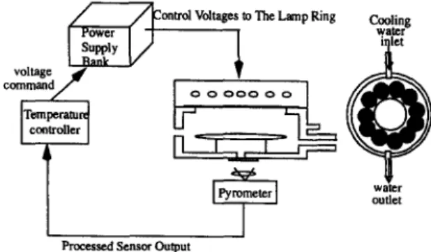
Fig. 3. Schematic of the closed-loop RTP system. Two quartz plates separate the lamps from the lower

half of the oven. The wafer rests on three quartz pins above the black water cooled oven floor. The side walls of the bottom half o f the oven are partially re- flective and are at an angle to the vertical. A pyrometer views the bottom surface of the wafer through a central hole in the floor.

Mathematical model of the closed-loop RTP system is described here. The model is called a global model because it simulates all the components in the RTP system and can thus be used to investigate the interplay of the control system with the heat transfer to the wafers as well as the thermal dynamics o f the wafer itself. A simplified schematic o f the closed-loop system is shown in Fig. 3. The system uses one bank of lamps which are arranged in orthogonal directions. The lamps are placed outside the reaction chamber's quartz windows. A flat reflector is located behind the bank of lamps. The system is controlled by a feedback control loop, which utilizes the difference between the converted temperature Tc and the set temperature Ts to control lamp power. The constituent components of the global model is shown in Fig. 4. The components include wafer thermal dynamic model (in particular, the heat transfer to and from the wafer) and lamp dynamic and my tracing model for the dynamics of lamp power to the wafer. A power supplier used to provide the power to lamps is also included. In the following, the mathematic model used for each component is described separately. These models are then integrated into a global model.

The approach employed is analytical/numerical in that the heat transfer to, from, and within the wafer is calculated. Included in the calculation is the radiation heat transfer to the wafer, the heat conduction

F

L

Feedback state

Thermal Radiati I

Ray T~cing Model

Corrected Pyrometer Measm~ Tempcratu~

Fig. 4. Global model components of the closed-loop RTP system.

within the wafer, and the heat convection and the heat loss emitted from the wafer surfaces. The present application is to low-pressure chemical vapor deposition (LPCVD). This process is typically at a pressure of 0.5-5 torr. At the densities associated with this pressure, convective cooling o f the wafer is secondary. Thus, convective cooling is not yet important. The present application is for temperature above 300°C, and hence the wafer is opaque to lamp radiation [15]. For the radiation, the heat from the lamps is absorbed at the wafer surface, and the radiant heat loss occurs at the surface.

As shown in Fig. 3, the controller sends a voltage command to the power amplifier after receiving mea- sured temperature signal from thermocouple (or pyrometer). The power reaches steady voltage level after receiving control voltage command in the ideal case. But in the actual situation, it is ramp up/down to reach the steady-state level. The lamp dynamics describes

(5)

C.-T Lin et al./Fuzzy Sets and Systems 103 (1999) 4945 53 the power from the lamps after receiving power supply

voltage. In most published papers, the dynamics of the lamp power intensity to the control voltage command was neglected, and the power from the lamps was assumed to be directly proportional to the power supply voltage. For this cause, we present a simple dynamic model between the command voltage and lamp power. The presented lamp dynamics has the following form:

V(t) : V(tk_l) -k- (comk -- V ( t k - l ) )

× ( 1 - e x p ( t - t k _ , ) )

"C

Plamp = f ( V ( t ) , T(x, t))" V(t) 2, (2) where V(t) is the power supply temporary voltage,

comk is the present command sent by the controller, tk-1 the last time step, Plamp is the lamp power, and the function f(V, T) is varied by V(t) and temperature

T(x, t) at position x. The presented lamp dynamics will raise the complexity of the RTP simulation, and match up the overall RTP system to actual RTP dynamics.

In our RTP system, electrical energy is supplied to a "ring" cylindrical arrangement of tungsten- halogen bulbs of which more will be mentioned later. Energy is radiated through a quartz windows onto a thin semiconductor wafer. A model of the heat transfer for such a system is developed in cylindrical coordinates, where the origin of the coordinate system is the center of the wafer bottom surface, and the z-axis of the coordinate system coincides with the central axis of the wafer. The model is based on the assumption that the temperature distribution is axi- symmetric and that the wafer is thin enough such that axial (z-axis) thermal gradients can be neglected. Fur- thermore, the wafer is discretized into annular zones in each of which the temperature is assumed to be uniform. Such an approach is often used in radiative heat transfer applications and has been used for RTP systems and for furnaces in [12].

The heat-transfer model of the wafer takes into account convective, conduction, and radiative energy transport mechanisms. The model is written as

]h = _ A r a d T 4 _ Aconv( T _ Ta) - - AcondT -~- BP, (3) where Ta is the ambient temperature expressed as an N × 1 vector (the ambient temperature is assumed to be constant in the chamber), T is the N × 1 tempera-

ture vector of the wafer elements, and P is the M × 1 lamp power vector, where N is the number of the wafer segments and M is the number of lamps [3]. The matrices Arad, Aeonv and Acond represent the radiative, convective, and conductive heat transfer, respectively. A complete description of these matrices can be found in [3]. The capacitive effects of the thick windows are neglected here, since the associated time constant is two-order magnitude larger than that of the wafer. Instead, the window heating model is considered as a slowly varying disturbance for the purpose of system identification and controller design. Physi- cal parameters used in the RTP model is the same as those used in [2].

3. SCAFIN-based adaptive control

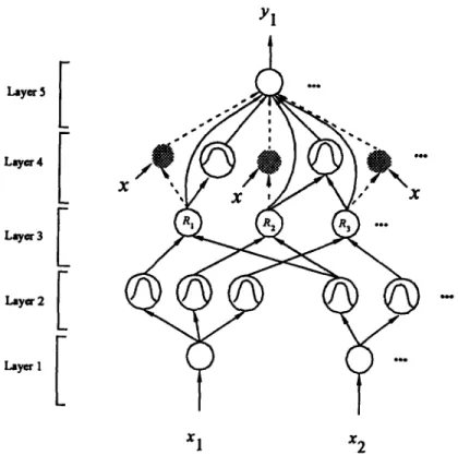
In this section, the structure of the SCAFIN as shown in Fig. 5 is introduced. With this five-layered network structure of the SCAFIN, we shall define the function of each node of the SCAFIN in Section 3.1, and the learning algorithm of the SCAFIN in Section 3.2.

3.1. Structure o f the S C A F I N

Let u (k) and a (k) denote the input and output of a node in layer k, respectively. The functions of the nodes in each of the five layers of the SCAFIN are described as follows.

Layer 1: No computation is done in this layer. Each node in this layer, which corresponds to one input variable, only transmits input values to the next layer directly, i.e.,

a (1) = u~ 1) =xi. (4)

Layer 2: Each node in this layer corresponds to one linguistic label (small, large, etc.) of one of the input variables in Layer 1. In other words, the membership value which specifies the degree to which an input value belongs a fuzzy set is calculated in Layer 2. With the use of Gaussian membership function, the operations performed in this layer is

( 2 ) 2 2

a(2) _ e-(Uu -mu)/~u, (5)

where mij and tr/j are, respectively, the center (or mean) and the width (or variance) of the Gaussian

(6)

54

C-T. Lin et aL /Fuzzy Sets and Systems 103 (1999) 4945

Y l Layer

5 I

Layer 4 I

Layer 3 I

Layer

2 I

Layer 1 I

x I x 2

Fig. 5. Structure of the proposed self-constructing adaptive fuzzy inference network (SCAFIN).

membership function of the jth term of the ith input variable x i. Unlike other clustering-based partitioning methods, where each input variable has the same number of fuzzy sets, the number of fuzzy sets of each input variable is not necessarily identical in the SCAFIN.

Layer 3: A node in this layer represents one fuzzy

logic rule and performs precondition matching of a rule. Here, we use the following AND operation for each Layer-3 node,

a(3) = H u~3)' (6)

i

where n is the number of Layer-2 nodes participating in the IF part of the rule.

Layer 4: This layer is called the consequent layer.

Two types of nodes are used in this layer, and they are denoted as blank and shaded circles in Fig. 5, respectively. The node denoted by a blank circle (blank node) is the essential node representing a fuzzy set (described by a Gaussian membership function) of the output variable. Only the center of each Gaussian

membership function is delivered to the next layer for the LMOM (local mean of maximum) defuzzification operation [6], and the width is used for output clustering only. Different nodes in Layer 3 may be connected to a same blank node in Layer 4, meaning that the same consequent fuzzy set is specified for different rules. The function of the blank node is

a(4) = Z

U~

"4)'aOi'

(7)

J

where aoi

=

moi, the center of a Gaussian membership function. As to the shaded node, it is generated only when necessary. Each node in Layer 3 has its own corresponding shaded node in Layer 4. One of the inputs to a shaded node is the output delivered from Layer 3, and the other possible inputs (terms) are the input variables from Layer 1. The shaded node function is

a = a.. j • ( 8 )

(7)

C.-72 Lin et aL / Fuzzy Sets and Systems 103 (1999) 49~55 55 where the summation is over all the inputs and

aji

is the

corresponding parameter. Combining these two types of nodes in Layer 5, we obtain the whole function performed by this layer for each rule as

a ( 4 ) : ( Z a j i x j + a o i ) U } 4 ) .

(9) J

Layer

5: Each node in this layer corresponds to one output variable. The node integrates all the actions rec- ommended by Layers 3 and 4 and acts as a defuzzifier with

a(5) (4) (10)

= ~ i ai

/ ~ . al 3)-

3.2. Learning aloorithms for the SCAFIN

Two types of learning, structure and parameter learning, are used concurrently for constructing the SCAFIN. The structure learning includes both the precondition and consequent structure identification of a fuzzy if-then rule. There are no rules (i.e., no nodes in the network except the input/output nodes) in the SCAFIN initially. They are created dynam- ically as learning proceeds upon receiving on-line incoming training data by performing the following learning processes simultaneously: (A) input/output space partitioning, (B) construction of fuzzy rules, (C) consequent structure identification, (D) parameter identification. In the above, processes A - C belong to the structure-learning phase and process D belongs to the parameter-learning phase. The details of these learning processes are described in the rest of this section.

A. Input/output space partitioning:

The way the input space is partitioned determines the number of rules extracted from training data as well as the number of fuzzy sets on the universal of discourse of each input variable. For each incoming pattern x, the strength a rule is fired can be interpreted as the degree the incoming pattern belongs to the corresponding cluster. For computational efficiency, we can use the firing strength given in Eq. (6) directly as this degree measure,

Fi(x)

= 1-[ u}3) : e--[Di(x--mi)]X[Di(x--mi)]' (11) i

where

F i C

[0, 1],

Di =diao(1/an, 1/ai2 ... 1lain),

and

mi = (rail, mi2 ... min ) T.

Using this measure, we can obtain the following criterion for the generation of a new fuzzy rule. Let

x(t)

be the newly incoming pattern. Find

J = a r g max FJ(x), (12)

1 <.j<~c(t)

where

c(t)

is the number of existing rules at time t. If

F J <~P(t),

then a new rule is generated, where

F(t)

6 (0, 1) is a prespecified threshold that decays during the learning process. Once a new rule is generated, the initial centers and widths are set as

m(c(t)+ 1 ) -~- x, (13)

= - ~ • diag(1/ln(Fg),..., 1~In(F J)),

D(c(t)+l) (14)

according to the first-nearest-neighbor heuristic [6], where fl/> 0 decides the overlap degree between two clusters.

After a rule is generated, the next step is to de- compose the multidimensional membership function formed in Eqs. (13) and (14) to the corresponding one-dimensional membership function for each input variable. For the Gaussian membership function used in the SCAFIN, the task can be easily done as

e--[Di(x--rai)]T[Di(x-mi)] = I X e--(xj-miJ)2/a~' (15)

J

where

mij

and aq are, respectively, the projected center and width of the membership function in each input dimension. To reduce the number of fuzzy sets of each input variable and to avoid the existence of redundant ones, we should check the similarities between the newly projected membership function and the existing ones in each input dimension. Since bell-shaped membership functions are used in the SCAFIN, we use the for- mula of the similarity measure,

E(A,B),

of two fuzzy sets, A and B, derived previously (see [7] for details), where

O<~E(A,B)<<.I

and the larger

E(A,B)

is, the more similar fuzzy set A is to B. Let ll(mi, ffi) represent the Gaussian membership function with center

mi

and width

ai.

The whole algorithm for the generation of new fuzzy rules as well as fuzzy sets in each input dimension

(8)

56 C-T. Lin et al./Fuzzy Sets and Systems 103 (1999) 49-65 is as follows. Suppose no rules are existent ini-

tially.

IF x is the first incoming pattern THEN do

P A R T 1.

{Generate a new rule,

with center ml = x, width D1 =

d iag( 1/ a init . . . 1/ ff init ),

where ffinit is a prespecified constant After decomposition, we have n one- dimensional membership functions,

with mli = xi and ~71i = ffinit, i = 1 • ' • n.

}

ELSE for each newly incoming x, do

P A R T 2.

{find J --- arg max1 <~j <~c(t) F J ( x ) , IF F J > / F i n ( t )

do nothing ELSE

{ c ( t + 1) = c ( t ) + 1,

generate a new fuzzy rule, with

1

mc(t+l ) = X, Dc(t+l) = - -~ . diag( 1/ln(F J) . . . 1 / l n ( F J)). After decomposition, we have

mnew_ i : X i , anew_ i : - - f l " ln(FJ), i = 1 . . . n . Do the following fuzzy measure for

each input variable i:

{degree(i, t) =- max1 ~<j~<ki E[lA( m n e w - i , a n e w - i ), I~( m j i , ff ji )],

where ki is the number of partitions of the ith input variable.

IF degree(i, t) <<. ~(t),

THEN adopt this new membership function, and set ki = ki + 1, ELSE set the projected membership function as the closest one.}

}.

In the above algorithm, ~(t) is a scalar similarity cri- teflon which is monotonically decreasing such that higher similarity between two fuzzy sets is allowed in the initial stage of learning. For the output space partitioning, the same measure in Eq. (12) is used. Since the criterion for the generation of a new output cluster is related to the construction o f a rule, we shall de- scribe it together with the rule construction process in Process B below.

B. Construction o f f u z z y rules: As mentioned in learning process A, the generation of a new input cluster corresponds to the generation o f a new fuzzy rule, with its precondition part constructed by the learning algorithm in Process A. At the same time, we have to decide the consequent part o f the generated rule. Suppose a new input cluster is formed after the presen- tation of the current input-output training pair (x, d), then the consequent part is constructed by the following algorithm:

IF there are no output clusters,

do { P A R T 1 in Process A, with x replaced by d} ELSE

do {

find J = arg maxj F J ( d ) . IF F J >>,Four(t)

connect input cluster c(t + 1 ) to the existing output cluster J ,

ELSE

generate a new output cluster,

do the decomposition process in P A R T 2 of Process A,

connect input cluster c(t ÷ 1) to the newly generated output cluster.

}.

The algorithm is based on the fact that the precon- ditions o f different rules may be mapped to the same consequent fuzzy set. Compared to the general fuzzy rule-based models with singleton output, where each rule has its own individual singleton value [11, 19], fewer parameters are needed in the consequent part of the SCAFIN, especially for the case with a large number of rules.

C C o n s e q u e n t structure identification: Up to now, the SCAFIN contains fuzzy rules in the form of Eq. (1). Even though such a basic SCAFIN can be used directly for system modeling, a large number of rules are necessary for modeling sophisticated systems under a tolerable modeling accuracy. To cope with this problem, we adopt the spirit o f the TSK model [17] into the SCAFIN. In the TSK model, each consequent part is represented by a linear equation of the input variables. It is reported in [17] that the TSK model can model a sophisticated system using a few rules. Even so, if the number of input and output variables

(9)

C-T. Lin et al./Fuzzy Sets and Systems 103 (1999) 4945 57 is large, the consequent parts used in the output are

quite considerable, some of which may be superflu- ous. To cope with the dilemma between the number of rules and the number of consequent terms, instead of using the linear equation of all the input variables (terms) in each rule, we add these additional terms only to some rules when necessary. The idea is based on the fact that for different input clusters, the corresponding output mapping may be simple or complex. For simple mapping, a rule with a singleton output is enough. While for complex mapping, a rule with a linear equation in the consequent part is needed. The criterion to deciding which type of consequent part should be used for each rule is based on computing

RE(i) = ~ t ~--~:1 a(3) a~3) (y(t) -- yd(t))2, (16)

where a~ 3) is the firing strength of rule i, c is the number of rules, yd(t) is the desired output, y(t) is the current output, and RE(i) is the accumulated error caused by rule i. By monitoring the error curve, if the error does not diminish over a period of time and the error is still too large, we shall add linear combinations of input variables to the rules whose RE(i) values are larger than a predefined threshold value.

D. Parameter identification: The parameter identi-

fication process is done concurrently with the structure identification process. The idea of backpropagation is used for this supervised learning. Considering the single-output case for clarity, our goal is to minimize the error function

E = ½ ( Y ( t ) - yd(t))2, (17)

where yd(t) is the desired output, and y(t) is the current output. The parameters, aji, in layer 4 are tuned by RLS algorithm as

a(t + 1 ) = a(t) + P(t + 1)u(t + 1)(yd(t) -- y(t)),

(18)

1 [ P(t)uT(t + 1)u(t + 1)P(t)]

P ( t + 1 ) = 2 L P ( t ) - 2 + u r ( t + 1 ) P ( t ) u ( t + 1)J'

(19) where 0 < 2 ~< 1 is the forgetting factor, u is the current input vector, a is the corresponding parameter

vector, and P is the covariance matrix. The initial parameter vector a(0) is determined in the structure learning phase and P(0) = aI, where a is a large positive constant. As to the free parameters mij and aij

of the input membership functions in layer 2, they are updated by the backpropagation algorithm. Using the chain rule, we have

0E m~2)(t + 1 ) = m~Z)(t) - rl dm~2 ) dE da (3) = m}Z)(t) - r/-ffy-y ~ ~y (20) Oak (3) ~3m}j 2)' where ~ y = y(t) - yd(t), Oy a(k 4) _ y da(3)ic v--, (3)

'

2-,i ai (21)

a(3) 2(xi -- mij)

k

₄

if term node j is connected to rule node k, 0 otherwise.

da' 3' {

dm}2 ) -- (22) Similarly, we have dE 6i5.2)(t -6 I) = 6i52)(t) -- r I Oy da k (23)

: tri~2)(t) -- r l

t~a~3) do-i~ 21'

where

[ a~3) 2(x a ? ij )2

Oak(3) _ / if term node j is connected ₍₂₄₎ t 3 ~ ) ] / to node k,

I, 0 otherwise.

3.3. Direct inverse control scheme

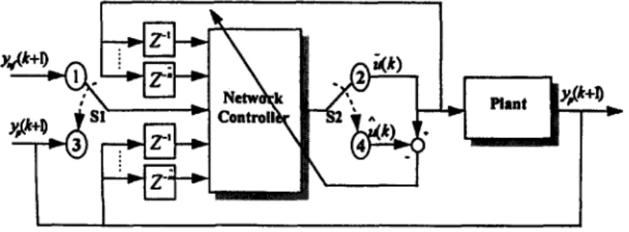
The direct inverse control configuration shown in Fig. 6 is adopted. Two training phases, off-line and on-line training, are used for the design of the controller. For the off-line training, the general inverse- modeling learning scheme [13] is used. A sequence

(10)

58 C.-T. Lin et al./Fuzzy Sets and Systems 103 (1999) 49-65

Fig. 6. Block diagram of the on-line training scheme.

of random input signals Urd(k) under the magnitude limits of the plant input is injected directly to the plant, and then an open-loop input-output characteristic of the plant is obtained. According to the input-output characteristic o f the plant, proper training patterns are selected to cover the entire reference output space. Using the collected training patterns with the values o f the selected input variables as the input pattern and the corresponding control signal Urd(k) as the target pattern, the network can be updated supervisedly to minimize an error function E defined

k,

b y E = ~ k = l l[Urd(k) -- u(k)] 2, where kn is the number o f training patterns, and fi(k) is the actual output of the training network.

For the on-line training, a conventional on-line training scheme is used. Fig. 6 is a block diagram for the conventional on-line training scheme. In execut- ing this scheme, we follow two phases, control phase and training phase. In the control phase, the switch S 1 and $2 are connected to node 1 and node 2, respectively, to form a control loop. In this loop, the control signal ti(k) is generated according to the input vector

I ' ( k ) = [yref(k+ 1 ), y p ( k ) , . . . , y p ( k - th+ 1 ), u ( k - 1 ),

. . . . u ( k - fi)]T, where u denotes the input, yp is the

output, and Yref is the reference output. In the training phase, the switch S1 and $2 are connected to node 3 and node 4, respectively, to form a training loop. In this loop, we can define a training pattern with input vector l ( k ) = [ y p ( k + 1 ) , y p ( k ) . . . . , y p ( k - th q- 1 ), u ( k - 1 ) . . . u ( k - t~)] T and desired output if(k), where the input vector o f network controller is the same as that used in the off-line training scheme. With this training pattern, the network controller can be trained supervisedly at each time step k to minimize the error function E ( k + 1) defined by

E ( k + 1) = ½[if(k) - fi(k)] 2, where fi(k) is the actual

output of the network controller when it receives the input vector I ( k ) in the training phase.

4. Simulation studies

4.1. R T P temperature control

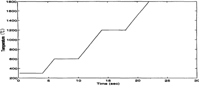
Fig. 7 shows a classical desired temperature profile for thermal process. The wide operating interval of 300-1800°C typically implies variable dynamics. The control objective is to control the temperature of the RTP system to follow the trajectory in Fig. 7.

Consider first that the lamp is located at the inner ring o f the wafer only. To design the multi- input-single-output (MISO) SCAFIN controller, both off-line and on-line training are adopted. In implementing the off-line training scheme, a sequence of random input signals Urd(k) limited between 0 and 1000 is injected directly to the simulated system described in Eq. (3). From the input-output characteristic of the simulated system (Fig. 8), 150 training patterns are selected to cover the entire reference output space. The input vector of the network controller is I ( k ) = [yp(k + 1 ), y p ( k )] T. We first tried the SCAFIN without linear terms added to the consequent part. Simulation results showed that such network could not learn the input-output relationship well, even that a large number of rules were used. The reason is that for similar inputs the desired outputs change sharply (Fig. 8) in this learning task. To han- dle this mapping, some additional terms selected via learning process C in Section 3.2 are added to the consequent part of the generated rules. The learning

(11)

C-T. Lin et al./ Fuzzy Sets and Systems 103 (1999) 49-65 59 1 8 0 0 1 6 0 0 1 4 0 1 ~ 1 2 0 0

~

1 0 0 0 e O 0 6 0 0 4 0 0 2 0 0 0

/

! 6

/

2S 1 0 1 6 2 0 T i m e ( s a c ) Fig. 7. Typical desired temperature profile.

3 0 2 0 0 0 ~ 1 5 0 0

~

1 0 0 0 6 0 0 5 1 0 1 5 2 0 2 5 3 0 t i m e ( s e c ) 1 0 0 0 I

6°° I

"~ 6 0 0 !

:oo

0 0 t i m e ( e e c ) 3 0

Fig. 8. Collected training data for inverse control, where the upper plot is y(k) and the lower one is u(k).

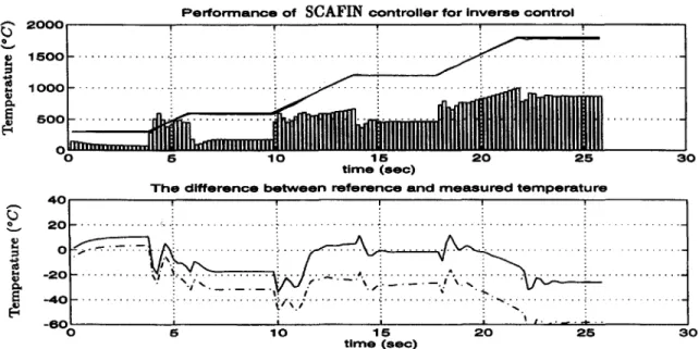
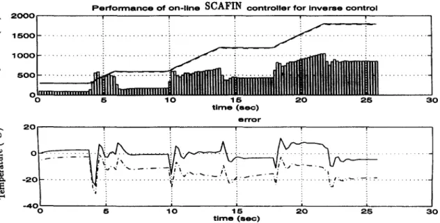
parameters in the SCAFIN are set as r/=0.005, fl = 0.5, Fin = 0.005, Pout = 0.7, and 2 = 0.96. After 20 epochs of off-line training, the controlled result is shown in Fig. 9. Fig. 10 illustrates the distribution of the training patterns and the final assignment of fuzzy rules in [y(k),

y(k

+ 1 )] plain. Eight rules are generated, with additional linear terms generated on four o f them during learning, and the number of fuzzy

sets on

y(k) and y(k

+ 1) are 5 and 5 (Fig. 11), respectively. To obtain a better result, on-line learning is also performed. After 5 epoches of on-line training, the controlled result is shown in Fig. 12. A better result is achieved.

To give a more clear understanding of the performance, comparisons with other controllers are made. They include the backpropagation (BP) neural

(12)

60 C.-T. Lin et al./Fuzzy Sets and Systems 103 (1999) 49-65 1 0.9 P e r f o r m a n c e o f S C A F I N c o n t r o l l e r f o r I n v e r s e c o n t r o l 2 0 0 0 ! 5 o 0 . . . i . . . 2

... ~

"

~ ...

o o o . . . i . . . . . . : . . . :: .. . . ' !i ~ ii "

! |111111111111

~OOio~,

... i ~ l l l l l l l n l l l l l ... 6" . . . 1 "0 " " 1 "15 . . . 2 0 2 5 3 0 t i m e ( $ e c ) T h e d i f f e r e n c e b e t w e e n r e f e r e n c e a n d m e a s u r e d t e m p e r a t u r e 4 0 2 0 : o - 2 0 f~ - 4 0 - 6 o o

...

i ...

... !

...

... ... ... ... : "~ . . . . ~V " i ' " i . . . ," " " - k v - : . . . : - "~/~-; . . . ~ .. . . i .... .~. . . ! . . . I I I I I I" . . ~ - , - i - - . 15 1 0 1 5 2 0 2 5 3 0 t i m e ( s e e )

Fig. 9. Performance of SCAFIN controller for inverse control; solid: center measurement, dashdot: marginal measurement.

+6 0.8 0.7 0.e ~o~ 0.I 0.~ 0.2 0.! 0.1 02 0.3 4 0.5 06 0.7 0.8 09 y~)

Fig. 10. Final learned fuzzy rules of SCAFIN inverse controller.

network based direct inverse control [ 13], model reference adaptive control ( M R A C ) [1], and proportional- derivative (PD) control. For the MRAC, the plant is identified with an AutoRegressive eXogenous ( A R X ) model, and a state-space approach control based on the identified model is employed. For the BP controller after extensive off-line training, the number

o f on-line training epoches performed on it is the same as that for the SCAFIN, which is five in total. The controlled results using PD, MRAC, and BP are shown in Figs. 13-15, respectively. Detailed comparisons, including the nonuniformity (n.u.f), maximum positive error, maximum negative error, and mean square tracking error, o f these controllers are made in Table 1. In Table I, the nonuniformity is defined as the mean square error between the wafer center and marginal measurements. The mean square tracking error refers to the error between the reference and wafer center measurements.

4.2. Improvement of temperature uniformity

From the above MISO controlled results, we ob- serve that the temperature gradient difference between the inner and outer rings o f wafer is not small. To obtain uniform processing across the wafer surface and to prevent the creation o f slip defects due to the thermal stress, the temperature must be nearly uniform across the wafer at all times. It is known that the distribution o f energy from the lamp or lamp array o f an RTP system must be nonuniform over the wafer to obtain uniform temperature distribution due to the radiative loss by the wafer edge and nonuniform

(13)

C.-T. Lin et al./Fuzzy Sets and Systems 103 (1999) 49-65 61 1 0 . 8 0 . 6 0 . 4 0 . 2 0 1 0 . 8 0 . 6 0 . 4 0 . 2 0 f i n a l M F e o n y ( k ) ' ~ f ' , 0 0 . 2 0 . 4 0 . 6 0 . 8 1 f i n a l M F s o n y ( k ÷ l )

'yj

0 0 . 2 0 . 4 0 . 6 0 . 8 1

Fig. 11. Final learned membership functions of SCAFIN inverse controller.

~-~ 2 0 0 0 P e r f o r m a n c e o f o n - l i n e SCAFIN c o n t r o l l e r f o r i n v e r s e c o n t r o l 1 5 0 0 n - i 1 0 0 0

i iiiiill

...

~ 0 5 1 0 1 6 2 0 2 5 t i m e ( e e o ) e r r o r 2 0 3 0 o -2(~ E

-4o~

. . . i . . ~ . . . : - - . : - , : , ' . ' . . . i . j : ~ . . ~ . . ~ . . . i 5 1 0 1 5 2 0 2 5 3 0 t i m e ( e e c )

Fig. 12. Improved performance of MISO SCAFIN controller after on-line learning; solid: center measurement, dashdot: marginal measurement.

convective cooling. If the distribution of lamp energy used during transients is simply a scaled version of what provides steady-state temperature uniformity, serious temperature nonuniformity will occur during transients. For most processes, it is of paramount im-

portance to avoid temperature gradients during both transients and steady states. Wafer edge irradiation has therefore to be adjusted versus experimental con- ditions. For that purpose, various means have been suggested, as for example, modification of reflector

(14)

6 2 C - T Lin et al./Fuzzy Sets and Systems 103 (1999) 4 9 ~ 5 r~ 1 5 0 0 1 0 0 0 5 0 0 0 T e m p e r a t u r e t r a c k i n g t r a j e c t o r y o f P D c o n t r o l 0 5 1 0 1 5 2 0 2 5 3 0 T h e d i f f e r e n c e b e t w e e n r e f e r e n c e a n d m e a s u r e d t e m p e r a t u r e 5 0 . . . . . o . . . . - : . . . ' . . . . . . . . . : . . . . . : . . . . . . . . ' . . . . ' ' t - * ' ~ - 5 0 . . . ~ ~ . . . . - - , . ~ . / ' ! - 1 O O I - . . . ! . . . ! . . . . - - " " - - ' - -i . . . : " ~ - - - L , - . . . . ? . . . -1 !50 0 5 1 0 1 5 2 0 2 5 3 0 F i g . 13. P e r f o r m a n c e o f P D c o n t r o l l e r ; solid: c e n t e r m e a s u r e m e n t , d a s h d o t : m a r g i n a l m e a s u r e m e n t . T e m p e r a t u r e t r a c k i n g t r a j e c t o r y o f t r a c k i n g s y s t e m 1 5 0 0 . . . • . . . + . . . • - : ; : t o o o . . . ~ . . . ! . . . i .. . . ::: ... 5 0 0 o ' . . . ...~ ... ; " " :: . . . . 0 5 1 0 115 2 0 2 5 3 0 T i m e ( s a c ) T h e d i f f e r e n c e b e t w e e n r e f e r e n c e a n d m e a s u r e d t e m p e r a t u r e 4 0 . . . . . . . . . . . . . . . . . . . . . 0 ' - . . . . , _ . . . ! . . . J - ~ . . ! - 2 0 . . . .. -- : • • .&!.-,~ . . . • ~: ~ I ! : ~ i ! : ~ - ~ : - 4 0 . . . : : " . . . ~ ! . . . i." .... i .. . . :: . . . -6t~ _-( i i i i i 5 1 o 1 5 2 0 2 5 3 0 T i m e ( s a c ) F i g . 14• P e r f o r m a n c e o f m o d e l r e f e r e n c e a d a p t i v e c o n t r o l l e r ( M R A C ) f o r t r a c k i n g c o n t r o l ; solid: c e n t e r m e a s u r e m e n t , d a s h d o t : m a r g i n a l m e a s u r e m e n t •

characteristics, special lamp arrangements, individual lamp powering, or mechanical movement o f the wafer. Thermal gradients m a y also be reduced by using either guard rings or suspector, i.e., by virtu- ally extending the wafer edge; this technique will be

applied in our RTP system later. Finally, instead o f using guard ring, we will present how to use the multi- input-multi-output ( M I M O ) S C A F I N to control the lamps' power individually to improve temperature uniformity.

(15)

C . - T . L i n et a l . / F u z z y S e t s a n d S y s t e m s 103 ( 1 9 9 9 ) 4 9 ~ 6 5 63 ~ - ~ 2 0 0 0 r ~ B P - B a s e d I n v e r s e c o n t r o l l e r I T : i 1 5 o o . . . ~ . . . ~ : - i - i - . . . i . , , d ' ~ :. . " i l o o o . . . : . . . i . . . ~ : . . . i . . . i . . . 5 0 0 2 1 k l . . . . . . . . . . . . . . . . . . . O ~ 0 5 1 0 1 5 2 0 2 5 3 0 t i m e ( s e e ) t r a o k e r r o r 5 0 ~ . . . . i . . ; . . , ~ . . . _ . . . ~ . . : : . : ~ . . _ ~ o . ~ ! .. . . ! . . . ........ ....................... - 1 o o i 5 1 0 115 2 0 2 5 3 0 t i m e ( s e e )

Fig. 15. Performance of baekpropagation (BP) network controller for inverse control; solid: center measurement, dashdot: marginal measurement.

Table 1

Summary table o f performance index

MIMO MISO MISO BP MRAC PD control

SONF1N SONFIN 0.0133 449.4375 446.2482 350.4692 436.2865 136.5641 135.7573 86.5752 74.5269 6.0851 10.5223 37.2696 4 . 6 9 E - 0 4 - 16.2234 - 18.4636 -35.2887 -37.8156 8.2991 46.1927 183.1709 521.6536 Nonuniformity (nut')

n u f at guard ring covered wafer

Maximum tracking error 5.1086

Minimum tracking error - 9 . 6 6 3

Tracking MSE 12.6401

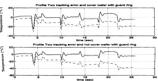
To avoid the edge heat loss, the general approach is adding the guard ring on wafer border to lengthen wafer radius. The edge loss radiation energy of the wafer will be reflected by the guard ring and the difference between the center and edge energy will be reduced. However, this method avoids the temperature gradient limitedly and is not suitable for improving the nonuniformity caused by the lamp radiation. The effect of using guard ring is simulated here. In Fig. 16, we show the improvement of temperature uniformity under the MISO SCAFIN inverse control for the wafer covered with guard ring. Such improvement statuses for all types of controllers discussed above are listed in Table 1.

For temperature uniformity and tracking, it is difficult for a single-output controller to reach these two claims simultaneously. The motivation of uniformity improvement is to add a circular bank of lamps over the wafer border to compensate the edge loss effect of the wafer. The lamps emphasize the incident radiation energy on the wafer edge and also adds the energy at the center. Two well-balanced lamp power sources usually cannot achieve the desired temperature and temperature uniformity simultaneously. Hence, a M1MO controller is required to control the power of different lamps individually. In the conventional control, it is difficult to overcome the MIMO control problem, especially for the nonlinear plant

(16)

64 C.-T. Lin et al./Fuzzy Sets and Systems 103 (1999) 49-65 2 0 P r o f i l e T w o t r a o k i n g e r r o r a n d c o v e r w a f e r w i t h g u a r d r i n g ! ! . . ~ . . ! . . . " . . . . ;v: ' . . . . . , , i . . . . , : , : - ~ , o . . . • , . . ~ . . . - ~ : , : . . . ~. . . ~ .. . . : : , - . . - . . . . . i m 4 0 / i 5 1 0 1 5 2 0 2 5 3 0 t i m e ( s e c ) . P r o f i l e T w o t r a c k i n g e r r o r a n d n o t c o v e r w a f e r w i t h g u a r d r i n g 2 0 *,...., o - 2 0 E - 4 c -eo~ ! ! !

.... ,,i ,, . . .

i ,

! ...

. . .

. . . . . . . . . , . . . |# I 1 I . . . : . . . ¢ : . , * . ' . - : ' . . ' . ' 7 " . : . . . I 15 1 0 1 5 2 0 2 5 t i m e ( e e c ) 3 0

Fig. 16. Comparison of temperature uniformity of the wafer with and without guard ring; solid: center measurement, dashdot: outer measurement. S C A F I N O n - l i n e l e a m l n g p e r f o r m a n c e 2 0 0 0 T ,~o0 ... ~ ... ~ ... i

... /

~

...

0 5 1 0 1 5 2 0 2 5 t i m e ( s e c ) ~ " 2 0 1 0 ~. o I~ -lO i - 2 o c e r r o r ! / !i. -" i . t , :,. i~.... . . • ~ . - ~ . - - , . - " . ~ . . - - ~ . . . I..~ . . . . ~ . ~ . . . i ~ - . - . ~ - , . . J . . . . - - , 7 . . . , . - : . . , - - . , . - - - . . - - ~ - . ~ . , - ~ - - : . . . ; ~'-," . . . i ! ~ . . . t! i i 15 1 0 115 2 0 2 5 3 0 t i m e ( 8 e o )

Fig. 17. Improved performance of MIMO SCAFIN controller after on-line learning; dotted: center measurement, dashdot: marginal measurement.

control. Nevertheless, the S C A F I N supports the fit- ness o f M I M O control.

W e add a circular bank o f lamps over the edge o f the wafer. The p o w e r range o f the edge lamps is the same

as that o f the central lamps. To generate the training data, 150 random signals [ue(k), uo(k)] (u¢(k) is the inner lamp p o w e r and uo(k) is the outer lamp p o w e r ) are injected directly to the plant described in Eq. (3).

(17)

C-T. Lin et al./Fuzzy Sets and Systems 103 (1999) 49-65 65 The 150 generated training patterns are used to train

the S C A F I N , with [yi[k],yi[k + 1],yo[k],yo[k + 1]] (Yi is the temperature at center ring and Yo at outer ring) being the inputs and [ue(k), uo(k)] the desired outputs. Eight rules are generated after 22 epochs o f off-line learning. Five and six linear terms are added to output uo and ue, respectively. After 14 epochs o f on- line training, the controlled result is shown in Fig. 17. M u c h better temperature uniformity is achieved. Detailed temperature uniformity comparisons are listed in Table 1.

5. Conclusion

A n adaptive fuzzy inference network, SCAF1N, with on-line self-constructing capability is proposed in this paper. The S C A F I N is a general connectionist m o d e l o f a fuzzy logic system, which can find its optimal structure and parameters automatically. Both the structure and parameter identification schemes are done simultaneously during on-line learning, so the S C A F I N can be used for normal operation at any time as learning proceeds without any assignment o f fuzzy rules in advance. Simulation results in temperature control o f the RTP system has verified its effectiveness.

Reference

[1] K.J. Astrom, B. Wittenmark, Adaptive Control, Addison- Wesley, Reading, MA, 1989.

[2] T. Breedijk, Model Identification and Nonlinear Predictive Control of Rapid Thermal Processing Systems, Ph.D. Dissertation, University of Texas at Austin, 1994.

[3] Y.M. Cho, T. Kailath, Model identification in rapid thermal processing systems, IEEE Trans. Semicond. Manuf. 6 (3) (1993) 233-245.

[4] J.S. Jang, ANFIS: adaptive-network-based fuzzy inference system, IEEE Trans. System Man Cybemet. 23 (3) (1993) 665 -685.

[5] C.C. Lee, Fuzzy logic in control systems: fuzzy logic controllers - Parts I, II, IEEE Trans. System Man Cybemet. 20 (1990) 404-435.

[6] C.T. Lin, C.S.G. Lee, Neural-network-based fuzzy logic control and decision system, IEEE Trans. Comput. 40 (12) (1991) 1320-1336.

[7] C.T. Lin, C.S.G. Lee, Neural Fuzzy Systems: A Neural-Fuzzy Synergism to Intelligent Systems (with disk), Prentice-Hall, Englewood Cliffs, NJ, 1996.

[8] C.J. Lin, C.T. Lin, Reinforcement learning for ART-based fuzzy adaptive learning control networks, IEEE Trans. Neural Network 7 (3) (1996) 709-731.

[9] H.A. Lord, Thermal and stress analysis of semiconductor wafers in a rapid thermal processing oven, IEEE Trans. Semicond. Manuf. 1 (3)(1988) 105-114.

[10] W.T. Miller III, R.S. Sutton, P.J. Werbos (Ed.), Neural Networks for Control, M.I.T. Press, Cambridge, MA, 1990. [11] J. Nie, D.A. Linkens, Learning control using fuzzified self-

organizing radial basis function network, IEEE Trans. Fuzzy Systems 40 (4) (1993) 280-287.

[12] S.A. Norman, Optimization of transient temperature uniformity in RTP system, IEEE Trans. Electron Devices 39 (1) (1992) 205-207.

[13] D. Psaltis, A. Sideris, A. Yamamura, A multilayered neural network controller, IEEE Control System Mag. 10 (3) (1989) 44 -48.

[14] F. Roozeboom, N. Parekh, Rapid thermal processing systems: a review with emphasis on temperature control, J. Vac. Sci. Technol. B 8 (1990) 1249-1259.

[15] T. Sato, Spectral emissivity of silicon, Jpn. J. Appl. Phys. 6 (3) (1991).

[16] F.Y. Sorrel, Temperature uniformity in RTP furnace, IEEE Trans. Semicond. Manuf. 39 (1) (1992) 75-80.

[17] T. Takagi, M. Sugeno, Fuzzy identification of systems and its applications to modeling and control, IEEE Trans. System Man Cybernet. 15 (1) (1985) 116-132.

[18] J. Tanomara, S. Omatu, Process control by on-line trained neural controllers, IEEE Trans. Indus. Electron 39 (6) (1992) 511-512.

[19] L.X. Wang, Adaptive Fuzzy Systems and Control, Prentice- Hall, Englewood Cliffs, N J, 1994.