財政政策與主權債務危機 - 政大學術集成

全文

(1)國立政治大學社會科學院經濟學系碩士論文 Department of Economics College of Social Sciences National Chengchi University Master Thesis. 治政財政政策與主權債務危機大立. The Sovereign Risk and the Fiscal Policy. ‧. ‧ 國. 學 y. Hsiao, Han-Ping. n. al. er. io. sit. Nat. 蕭瀚屏. Ch. engchi. i n U. v. 指導教授：黃俞寧博士 Advisor: Hwang, Yu-Ning, Ph.D. 中華民國一百年七月 July, 2011.

(2) 謝詞. 在政大就讀碩士的這兩年，經歷了許多以前不會面臨的困難，也因此讓我收穫良多。非常感謝黃俞寧老師如此用心的指導我如何撰寫碩士論文，且在我遇到研究上的困難時，非常耐心的指點我。並循序漸進的教會我如何找尋問題、定義問題與解決問題的方法。讓我受益良多。也感謝口試評審委員世新大學張淑華老師與國立嘉義大學張瑞娟老師，有你們的指點，才能使這篇論文內容更為豐富、更為嚴謹。. 政治大的時候，提供我很大的幫助。也時常在我撰寫論文遇到問題的時候，不吝給予我立. 另外要感謝碩班的朋友們。朱詩閔、賴柏勳與林銘峰，在我研究上面臨瓶頸. 指點。張慈恬、蕭宇翔和彭竣永，在課業上給予我很大的幫助。呂暉鵬、陳敬翔、. ‧ 國. 學. 潘葛天與謝育霖在我煩悶的時候會陪伴我，讓我減輕壓力。. ‧. 再來特別要感謝經濟系系桌的朋友們，陪伴我度過碩士班兩年的時間。尤其. y. Nat. 是陳怡文和陳玉桐，在我撰寫論文遇到困難的時候，會鼓勵我為我打氣。在我電. er. io. sit. 腦遇到問題的時候，不吝嗇的借出電腦以供我使用。在我煩悶需要紓壓的時候，即使你們再忙，也會撥時間陪伴我。有你們的支持，才能讓我順利的完成碩士學. n. al. 位。. Ch. engchi. i n U. v. 最後要感謝我的父母。雖然在碩士的生活我幾乎是在學校度過，但因為有你們在背後無私的支持與鼓勵，才能成就今天的我。真的謝謝大家給予我的關心與指點，讓我不僅在碩士、甚至是往後的人生，都有很大的幫助與鼓勵。有大家的陪伴，才能使我完成這篇論文。僅將此篇論文獻給我的父母、朋友與老師。蕭瀚屏. 謹誌. 政治大學經濟學系碩士班中華民國一百年七月 I.

(3) 中文摘要. 在次級房貸風暴之後，各國赤字大幅增加。如希臘與愛爾蘭，其主權債務違約風險皆大幅升高。面對這樣的困境，政府該如何實施財政政策，以防止主權債務危機的發生?本篇文章在 DSGE 模型之下，以 Uribe(2006)的設定為基礎架構，額外增加了產出方程式以使國家產出能由模型內生決定。並加入了政府支出與產出之間的關係式，以討論在面對正的景氣衝擊與負的景氣衝擊時，政府使用正向景氣循環政策和負向景氣循環政策對於政府倒債率的影響。最後發現當政府使用. 政治大反向的關係。而當政府使用較強的順向景氣循環政策時，政府的倒債率會和技術立. 負向景氣循環政策和較弱的順向景氣循環政策時，政府的倒債率會和技術衝擊有. ‧ 國. 學. 衝擊有正向的關係。從此結果，我們推論在後金融海嘯時期，希臘與愛爾蘭等國家，應使用較強的順景氣循環政策以降低其主權債務危機的發生機率。. ‧. n. al. er. io. sit. y. Nat. 關鍵字: DSGE、財政政策、主權債務危機. Ch. engchi. II. i n U. v.

(4) Abstract. After the subprime crisis, many government deficits rose sharply, especially Greece and Ireland. Their default rate rose greatly than before. Under this difficult situation, what kind of fiscal policy should the government enforces to prevent it from bankruptcy? We follow the model in Uribe (2006) as our framework but adding the production function and the government expenditure function to analyze the effects of different fiscal policies on the government default rate. The results tell us that when. 政治大 the change of the default rate is opposite to the technical shock. On the contrary, when 立. the government uses countercyclical fiscal policy and weak procyclical fiscal policy,. the government uses strong procyclical fiscal policy, the default rate is positive. ‧ 國. 學. relation with the technical shock. This implies that governments, such as Greece and. ‧. Ireland, should use strong procyclical fiscal policy to reduce their sovereign risk. n. al. er. io. sit. y. Nat. under the recession.. Ch. Keywords: DSGE、fiscal policy、sovereign risk. engchi. III. i n U. v.

(5) Contents 1. Introduction…………………………………………………………………………1 1.1 Motivation………………………………………………………………………1 1.2 Literature review………………………………………………………………..2 2. The model…………………………………………………………………………...7 2.1 Household……………………………………………………………………….7 2.2 The fiscal authority………………………………………..……………………9 2.3 Equilibrium………………………………………………………………...….10. 政治大 3.1 The countercyclical and procyclical fiscal policy…………………………..…14 立. 3. Discussion……..........….…………………………..………………………...……14. 3.1.1 The relationship between τ and g ………………………………...…....14. ‧ 國. 學. 3.1.2 The relationship between δ t and ε A,t …………….…………………...…15. ‧. 3.2 Other factors and the policy implication………………………...………….....16. sit. y. Nat. 4. Conclusion………………………………………………………………………....19. n. al. er. io. Reference……………………………………………………………………………..20. i n U. v. Appendix ………………………..………………………………………...………….21. Ch. engchi. IV.

(6) 1. Introduction 1.1.. Motivation In the middle of 2007, the subprime crisis began. This made the American. economy fall into recession. Due to the derivatives traded worldwide, this crisis affected not only the U.S. but other countries in the world. In response to the crisis, many governments use the fiscal tools to help the banks and financial system from crash. The fiscal expansion causes the quick accumulation of public debts. As a result, some governments went into financial difficulty. Iceland even went bankrupt in 2009.. 政治大 of them issued lots of debt to relieve the pressures of recession. With the great deficits, 立 The same scenario also occurred to other Europe countries, Ireland and Greece. Both. the possibility of government’s default surged. Other countries such as the US, Spain. ‧ 國. 學. and Portugal also face the same risk. Finally they have to seek the assistance from. ‧. IMF and the European Union. The debt risk has demonstrated the close relationship. sit. y. Nat. between the possibility of government’s default and the government expenditure. io. out the factors that make the governments turn insolvent.. al. er. without well control of the debt issues. This is the main reason that we want to find. n. v i n C hdefault rate was studied The issue of the government’s by Uribe (2006). He tried engchi U. to obtain the default rate endogenously to explain the Argentine debt crisis in 2001. The Argentine debt crisis occurred due to the failed monetary policy that pegged the peso/dollar exchange rate. With the fear of government payment ability, the Argentine government defaulted eventually. The author sets up a DSGE model to discuss about the default rate with different specifications of monetary policies such as the Taylor rule, price targeting, and exchange rate targeting. Under these monetary-fiscal regimes the government inevitably defaults. However, there is no government spending and the output is exogenous in his model. By using the model in Uribe (2006) with the endogenous output and government 1.

(7) expenditure, we want to investigate how the default rate may vary with different public spending. Particularly, we want to analyze the impacts of procyclical and countercyclical fiscal policies on the default rate. This is useful for the government to consider how to maintain the low sovereign risk while taking the expansionary fiscal policy. It is also useful for the investors to distinguish which country may have a potential risk to default. Here, we state the results briefly. The fiscal policies do have effects on the default rate. When it is countercyclical fiscal policy, the government default rate will. 政治大 procyclical fiscal policy, which means the government spending responded to the 立. have negative relation with the technical shock. When the government applies weak. output is smaller than the income tax rate, the default rate will also be negative. ‧ 國. 學. relation with the technical shock. But when the government uses strong procyclical. ‧. fiscal policy, which means the government spending responded to the output is larger. sit. y. Nat. than the income tax rate, the default rate will be positive relation with the technical. io. er. shock. The initial deficits also affect the default rate. A country with higher initial deficits will face a higher default rate.. al. n. v i n This paper is organized asCfollows. The first section h e n g c h i U is the motivation and the. questions that we want to analyze and the literature review. The second section is the model setting which extends the model of Uribe(2006). In the third section, we. discuss the results which were derived from the model and the last section is the conclusion.. 1.2.. Literature review The government default is not a new topic to economics. People usually think. that the government will not crash, but these scenarios never stop happened. From the book “This Time is Different” which states the history of country’s bankruptcy, we 2.

(8) can see that even the advanced countries such as England, the US, have defaulted several times in the history. But the issue of government default was never discussed until it suddenly happened. The research about the government default has been studied from different points of view. Caballero and Krishnamurthy (2004) talked about the reasons why countercyclical fiscal policies are fine in some countries during crises but resulted in bankruptcy in other countries. They assume that during an external crisis, the supply of funds is constrained and thus has limited financial depth. Therefore, the. 政治大 the government borrows the less the private sectors invest. The situation is more 立 crowding-out effect occurred. In other words, with the limit available fund, the more. severe in emerging countries than that in advanced countries. The reason is that the. ‧ 國. 學. author sets the available funds is affected by the level of the government credit. When. ‧. the government is responsible for its debt, the investors will supply more funds. When. sit. y. Nat. the government has no fiscal discipline, the investors will reduce the borrowing.. io. er. Because of the constrained funds, the crowding-out effect was even large during the crisis than during the normal time. This situation lessens the effects of expansionary. al. n. v i n C hcrash. However, inUthe reality, the reduction of the fiscal policy and finally runs into engchi. investments may not be entirely caused by the crowding-out effect. During the recession, the firm usually decreases its supply and lowers the investment for the next year. Therefore, the government needs to offset the private investments by the expansionary fiscal policy to maintain the aggregate demand for output. Moreover, this paper sets the government default rate as an exogenous factor. This is not true because the initial debt, the structure of the liabilities and the tax revenue will also affect the government payment ability. The disaster of default will happen not only during the crisis. Three papers discuss about the government default in the normal times include Romer (2006), 3.

(9) Uribe (2006) and Bi (2010). In Romer (2006), he sets up a model to characterize the government default rate. The author has two points. First, he thinks that the investors will borrow if the expected return rate equals to the risk-free interest factor. Second, the government will default if the tax revenue is not equal to the matured liability. There are two equilibriums in this model. The first equilibrium occurs when the interest rate is slightly above the risk-free interest rate and the possibility of default is very small. The second equilibrium occurs when the possibility of default is 1. This means that the investors will not borrow the money at any interest rate. This model. 政治大 happened for several reasons.. illustrates not only the government but also the investors’ behaviors. It clearly tells us that the government default. 立. On one hand, the. government foundations which are described by the distribution function of the tax. ‧ 國. 學. revenue will affect the probability of default. On the other hand, the exogenous. ‧. variables can also affect the probability of default. This means that even two countries. sit. y. Nat. with the same distribution function of the tax revenue will have different probabilities. io. er. of default. However, this model does not have government spending and lacks microeconomic foundation to determinant the quantity of available funds in the. n. al. equilibrium.. Ch. engchi. i n U. v. Uribe (2006) used another way to describe the issue of government default in the normal times. The author sets a Dynamic Stochastic General Equilibrium model that has micro-foundation for household and government. The household knows that there is the possibility that the government defaults a fraction of its liability if it does not have enough money to pay the interest. In the equilibrium we can derive the default rate endogenously. The formation of the default rate tells us that if the discounted sum of the expected tax revenue equals to the initial debt, then the government will not have to default even it has lots of deficits right now. The result is distinct from Romer (2006). Because in Romer (2006) the government will crash if its tax revenue is 4.

(10) smaller than its debt when the debt is due. In Uribe (2006), the payment-ability is measured through its life time. This means that the government will not default if the lifetime income is more than the lifetime deficit. The author continues to analyze the default rates under several monetary policies. When the central bank uses the Taylor rule as their monetary policy, the economy will have hyperinflation. When the central bank uses the price level targeting as their monetary policy, the government gives up its ability to inflate away part of the real value of its liabilities in response to the negative fiscal shocks. It turns out that the government can not peg the price without. 政治大 spending for simplification. Both of the assumptions are not consistent with the reality 立. default. But the author lets the output as a constant and assumes no government. and the results can be different if these assumptions are relaxed. With the growth of. ‧ 國. 學. economy, the government could afford more deficits. Hence, the assumption of the. ‧. output will definitely change the government payment ability.. sit. y. Nat. In the research of Bi (2010), the author considers the model similar to Uribe. io. er. (2006) that the government may partially default on its liability. In addition, this paper adds exogenous government expenditure, letting the tax rate endogenously. al. n. v i n C h lump-sum Utransfer countercyclical engchi. determined, and sets a. to households. These. assumptions make the model more close to the reality. The results show that the fiscal limits, which means the ability and willingness of the government to service its debt, is affected by the degree of countercyclical policy responses. The more lump-sum transfers level the more dispersed distributed the fiscal limits are. Finally the author finds a relationship between the default risk premium and the government debt, which is also found in Uribe (2006). Although the author has implemented the government spending, he sets it following a form of AR(1) which is not always right. In advanced countries the fiscal policy is usually countercyclical and the fiscal policy is procyclical in emerging countries. This phenomenon was found in Caballero and 5.

(11) Krishnamurthy (2004). Therefore, if we want to describe the relationship between the default rate and the fiscal policies more accurately, we should set the fiscal factors more carefully. The effects of fiscal policy were also discussed a lot in the previous literatures. The expansionary fiscal policy can stimulate the country economy, boost the demand, but it also results in accumulating the government deficits, raises the government bond premium. This is always a dilemma to every country to weigh gains and losses between the costs of government debts and the effects of expansionary fiscal policy.. 政治大 increase the deficits, the fiscal policy has great effects to boost the demand in the 立 Furceri and Mourougane (2009) used DSGE model to prove that although it will. short term. The increase in the public investment has the largest short-term effect. The. ‧ 國. 學. rise in the public consumption can also significantly affect the GDP. Tax cut is the. ‧. least effective in supporting the aggregate demand. In the paper of Devereux (2010). sit. y. Nat. also talks about the effectiveness of fiscal policy. But it sets the time during the crisis. io. er. that is usually accompanied by a liquidity trap. Under the liquidity trap, the government spending is more useful with deficit-financed than with tax-financed. The. al. n. v i n C hin the normal timeUcan also be highly expansionary tax cut that usually have no effects engchi in the liquidity trap.. Expansionary fiscal policy seems to have benefits to the economy but it also makes the country’s deficits increased. In the next section we will built a model of the relationship between the fiscal policy and the government default rate. Then, we will analyze what kind of fiscal policies will cause the default rate change.. 6.

(12) 2. The Model. 2.1.. The household Consider an economy with a large number of identical households, and the. preferences described by the utility function ∞. max Et ∑ β tU (ct , lt ). (1). t =0. Where ct denotes consumption of perishable goods and lt denotes leisure.. U (ct , lt ) denotes the single-period utility function, β ∈ (0,1) denotes the subjective discount factor, and. 政治大 E denotes the mathematical expectation operator conditional on 立 t. ‧ 國. 學. the information available in period t . The function U (ct , lt ) is assumed to be increasing, strictly concave, and continuously differentiable. In each period t ,. ‧. households distribute their wealth to consumption and labor supply to maximize their. sit. y. Nat. utility.. n. al. er. io. In each period, households have incomes, firm’s profits and interest rate from. i n U. v. government debts holding, as their wealth. But the government bonds are risky assets. Ch. engchi. that they may default for a percentage of the amount, denoted by δ t . Thus, the gross interest rate return in period t is denoted by Rt −1 Bt −1 (1 − δ t ) . Households earn incomes by offering their labor, but they have to pay a percentage of income for tax.. Bt denotes nominal government debts that households want to purchase in period t . In addition, this model is under the perfect competitive market which means that the firms’ profits is zero, thus we will not put the factor of firm’s profits in the budget constraint. Totally, we can derive the budget constraint of the household in period t as follows: 7.

(13) (1 − τ t ) Pw t t (1 − lt ) + Rt −1 Bt −1 (1 − δ t ) = Pc t t + Bt. (2). The right-hand side of the budget constraint represents the uses of wealth: consumption spending and the purchases of government bonds. The left-hand side of the budget constraint represents the received wealth: the real income after taxed and the interest rate return from government bonds. The household chooses the set of processes to (2), assume the set of processes. {ct , lt , Bt }t =0 ∞. {Pt , Rt −1 ,τ t , δ t , wt }t =0 ∞. to maximize (1) subject. as given. When we set the. lt ) ln ct + b ln lt , where b > 0 , and let the Lagrange utility function as U ( ct ,=. 立. 政治大. multiplier on the period t budget constraint be β t λt Pt . Then, use the Lagrange. ‧ 國. 學. method to solve the utility maximization we can get the following first ordering. io. (3). y. b λt wt (1 − τ t ). sit. λt. Nat. lt =. 1. ‧. ct =. n. al.  λt +1β t +1  λt β t Et  Rt (1 − δ t +1 ) = Pt +1  Pt . Ch. (4). er. conditions:. engchi. i n U. v. (5). Let the production function as. = yt At (1 − lt ). (6). This is one of the different assumptions to the Uribe(2006). In his paper, he sets the output as a constant in each period. Together with the goods market clearing condition:. y= ct + gt t. where gt is the government expenditure. (7). We can derive the consumption, labor supply and the Lagrange multiplier in terms of the exogenous variables (see Appendix 1): 8.

(14) ct =. (1 − τ t ) wt ( At − gt ) At b + (1 − τ t ) wt. (8). (1 − τ ) w + bgt 1 − lt = t t At b + (1 − τ t ) wt. λt =. (9). At b + (1 − τ t ) wt 1 (1 − τ t ) wt At − gt. 2.2.. (10). The fiscal authority In period t , the government expenditure is organized by the fiscal policies and. the interest rate, denoted by gt , Rt −1 Bt −1 respectively. The wealth of the. 政治大 τ . The government can accommodate its deficits by simplification, denoted by立 government comes from the income tax and we set the tax rate as a constant for. ‧ 國. 學. financing the government bonds which have to pay the interest Rt in the period t + 1 . Additional, we assume government bonds are risky assets. For each period the fiscal. ‧. authority may default on a fraction δ t of its total liabilities. With these assumptions,. er. io. sit. y. Nat. we can write the government budget constrain as follow. Bt =Pt gt + Rt −1 (1 − δ t ) Bt −1 −aτ Pw t t (1 − lt ). n. v ni. (11). l C The government spending is h another in this paper. Because in Uribe e n gkeyc point hi U. (2006), there is no government expenditure in the government budget constraint. Therefore, the result of the government default rate will not be affected by the fiscal policy. In order to analyze the effects of the different fiscal policy to the government default rate, we set the government spending as a response to the outputs, denoted as follow:. gt = gyt. (12). The factor g represents the type of the fiscal policies. When g > 0 means the government uses procyclical fiscal policy. The government will increase its spending 9.

(15) during the boom and reduce the expenditure during the recession. On the other hand, g < 0 implies the government uses countercyclical fiscal policy. It will reduce its. spending during the boom and expand its expenditure during the recession. In addition, the negative government expenditure can be seen as a tax which is levied by the government to compensate its deficits. By this assumption, we can show that the government default rate will be influenced by the fiscal policy. This topic will be discussed more detailed in the next section.. 政治大 In equilibrium, every market must be cleared. That means: 立 Equilibrium. At = wt. 學. y= ct + gt t. ‧ 國. 2.3.. (13) (14). ‧. Equation (13) is the goods market clearing condition. The output is determined. sit. y. Nat. by the consumption and the government spending. It is the most different from the. n. al. er. io. Uribe (2006) which has no government spending and takes the output as a constant.. i n U. v. Equation (14) is the labor market clearing condition which is derived from the. Ch. engchi. marginal product of labor equal to the real wage.. With the first order condition from household utility maximization, eq.(5), eq.(8), eq.(9), eq.(10), the government budget constraint, eq.(11), the assumptions for the production function and the government spending, eq.(6), eq.(12), and the market clearing conditions, eq.(13), eq.(14), we can define the equilibrium as follows:. Definition：The competitive equilibrium with rational expectation is a set of processes. {Pt , Bt , Rt , δ t , λt , wt , gt , lt }t =0 ∞. satisfying the following conditions:. 10.

(16) λt =. At b + (1 − τ ) wt 1 (1 − τ ) wt At − gt. (15). (1 − τ ) At + bgt 1 − lt = At b + (1 − τ ) At. (16).  P λ  1 Et  Rt (1 − δ t +1 ) t t +1  = Pt +1 λt  β . (17). Bt =Pt gt + Rt −1 (1 − δ t ) Bt −1 − τ Pw t t (1 − lt ). (18). lim β t + j +1λt + j +1 Et Rt + j (1 − δ t + j +1 ) j →∞. Bt + j Pt + j +1. = 0. (19). 政治大. Equation (17) is the Euler equation derived from the eq.(5). Equation (19) is the household transitivity condition.. 立. Now we started to derive the government default rate. First, multiplying the. ‧ 國. 學. left-hand and the right-hand sides of eq. (18) by Rt (1 − δ t +1 ) , we can rewrite the. ‧. equation as follow:. sit. y. Nat. Rt Bt (1 − δ t= Rt −1 Bt −1 (1 − δ t ) Rt (1 − δ t +1 ) + [ Pt gt − τ Pw +1 ) t t (1 − lt ) ] Rt (1 − δ t ). n. al. er. io. and iterating forward j times. Then we can get:. i n U.  j  Rt + j Bt + j (1 − δ t + j += ( Rt −1Bt −1 (1 − δ t ) ) ∏ Rt +h (1 − δ t +h+1 )  1)  h =0  j j   + ∑ ∏ Rt + k (1 − δ t + k +1 )  [ Pt + h gt + h − τ Pt + h wt + h (1 − lt + h ) ] h =0  k =h . Ch. engchi. Multiplying the above equation both sides by. β t + j +1λt + j +1 Rt + j. Bt + j Pt + j +1. = − δ t + j +1 ) β t + j +1λt Rt −1 (1. β t + j +1λt + j +1 Pt + j +1. v. one obtains:.  j  Bt −1 P λ (1 − δ t ) ∏ Rt + h (1 − δ t + h +1 ) t + h t + h +1  Pt Pt + h +1 λt + h   h =0. j  j  P λ + ∑ ∏ Rt + k (1 − δ t + k +1 ) t + k t + k +1 λt + h [ gt + h − τ wt + h (1 − lt + h ) ] β t + j +1 Pt + k +1 λt + k  h =0  k =h. For simplification, we use eq.(17) and forward h times. Then, we can have: 11.

(17) Rt + h (1 − δ t + h +1 ). Pt + h λt + h +1 1 = β Pt + h +1 λt + h. (20). Using eq.(20), we can rewrite the equation above the eq.20 as follows (see Appendix 2):. β t + j +1λt + j +1 Rt + j. Bt + j Pt + j +1. (1 = − δ t + j +1 ) λt Rt −1. j Bt −1 t β (1 − δ t ) + ∑ β t + h {λt + h [ gt + h − τ wt + h (1 − lt + h )]} Pt h =0. Applying the conditional expectations operator Et on both sides of this expression, taking the limit for j → ∞ , then we can get:. 政治大.   Bt + j B lim Et  β t + j +1λt + j +1 Rt + j (1 − δ t + j +1= )  λt Rt −1 t −1 (1 − δ t ) β t j →∞ Pt + j +1 Pt   ∞  + Et ∑ β t + h λt + h [ gt + h − τ wt + h (1 − lt + h ) ]  h =0 . 立. ‧ 國. 學 ‧. Using the eq.(19) one obtains:. y. sit. Nat. Bt −1  ∞ t +h  t λt R= (1 − δ t ) β Et ∑ β λt + h [τ wt + h (1 − lt + h ) − gt + h ] t −1 Pt  h =0 . n. al. er. io. Diving the above equation both sides by β t , then we can derive the government default rate as follow: ∞. ∑β. δ t = 1 − h =0. h. Ch. engchi. Et {λt + h [τ wt + h (1 − lt + h ) − gt + h ]}. i n U. v. (21). λt Rt −1 Bt −1 Pt. Using the eq.(12) we can obtain the relationship between the government spending and the technical rate(see Appendix 3):. gt =. g (1 − τ ) At (1 − τ ) + (1 − g )b. (22). With this equation, we can also get the form of the Lagrange multiplier as following equation(see Appendix 4):. λt =. (1 − τ ) + (1 − g )b 1 (1 − τ )(1 − g ) At. (23) 12.

(18) By the eq.(16) and eq.(22), we can also find the form of the labor supply which is a constant variable(see Appendix 5):. (1 − τ ) (1 − lt ) = (1 − τ ) + (1 − g )b. (24). Using the eq.(21), eq.(6) and eq.(12), we derived the following equation: ∞. δt = 1 −. ∑β h =0. h. Et {λt + h At + h (1 − lt + h )(τ − g )}. (25). λt Rt −1 Bt −1 Pt. Together with the eq.(23), eq.(24) and eq.(25), we can find the form of the government default rate as follow:. δt = 1 −. 政治大. (τ − g )(1 − τ ) 1 1 At [(1 − τ ) + (1 − g )b] (1 − β ) ( Rt −1 Bt −1 Pt ). 立. (26). = At ρ A At −1 + (1 − ρ A ) A + ε A,t. 學. ‧ 國. If we assume the technical rate as follow: where ε A,t is i.i.d.. (27). y. sit. io. (τ − g )(1 − τ ) 1 1  ρ A At −1 + (1 − ρ A ) A + ε A,t  [(1 − τ ) + (1 − g )b] (1 − β ) ( Rt −1 Bt −1 / Pt −1 ) . n. al. (28). er. δ t =1 −. Nat. as follow:. ‧. Then, we can get the closed form of the government in terms of exogenous variables. i n U. v. From this equation, we can see that the government default is affected by the initial. Ch. engchi. debts, the initial technical rate, the equilibrium technical rate, the error term of the technical rate, the tax rate and finally, the level of the government expenditure. Especially, the degree of the government spending is the main idea that we want to discuss. Thus, we will analyze the effect of the fiscal policy more detailed in the next section.. 13.

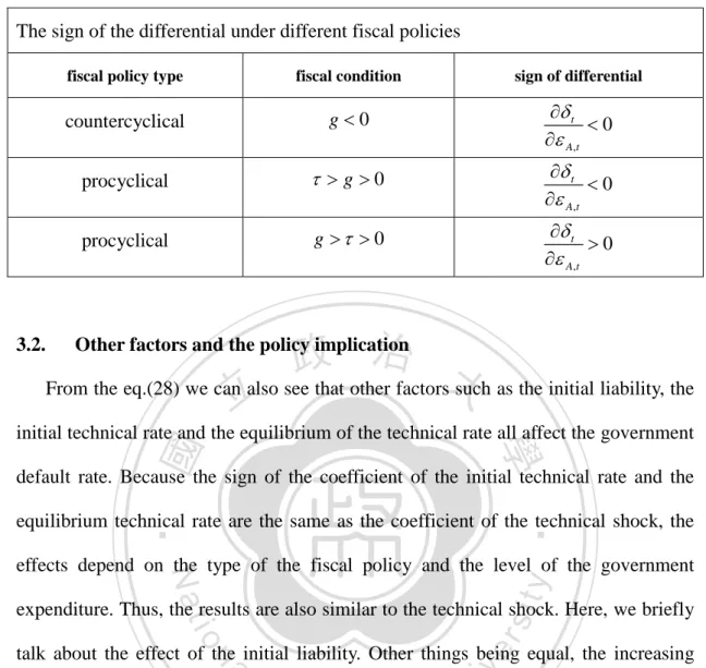
(19) 3. Discussion. We want to analysis the effects of countercyclical fiscal policy and procyclical fiscal policy on the government default rate. But the effects are not always the same. The different economic condition will change the effects of fiscal policies. Thus, as we set the technical shock represent the economic condition, during the boom the economy will face a positive technical shock and during the recession the economy will face a negative technical shock, we can analysis the change of the government. 政治大 section is as follows. First,. default rate under different kinds of fiscal policies. The organization in this. 立. we will discuss the. relationship between the government default rate and the technical shock under the. ‧ 國. 學. countercyclical and procyclical fiscal policy. Then, we will describe other effects that. ‧. also influence the government default rate. Finally, we will use the results to give. sit. The countercyclical and procyclical fiscal policy. n. al. Ch. 3.1.1. The relationship between τ and g. engchi. er. io. 3.1.. y. Nat. governments some policies implication during the boom and the recession.. i n U. v. The level of the tax rate and the fiscal response are very important factors that will be used in the next section. Thus, we use the government budget constrain under the steady state to find the limitation to τ and g . The results express as below (see Appendix 6):. B (1 −. 1. β. (1 − δ )) = P ( g − τ ) y. (29). Because the sign of government bonds can be positive or negative, this means that there is no restriction between tax rate and the fiscal response. In other words, the level of the fiscal policy can be either larger or smaller than the level of the income 14.

(20) tax.. 3.1.2. The relationship between government δ t and ε A,t Here, we differentiate the eq.(28) by the technical shock. We express this equation as below:.  (τ − g )(1 − τ )  1 ∂δ t 1 = −  ∂ε A,t  (1 − τ ) + (1 − g )b  1 − β Rt −1 Bt −1 Pt. (30). As we assume 1 > β > 0 and the initial debts are positive, the sign of the differential is decided by −. 政治大. (τ − g )(1 − τ ) . There are three possible outcomes which are: (1 − τ ) + (1 − g )b. 立. ∂δ t <0 ∂ε A,t. when τ > g > 0. ∂δ t >0 ∂ε A,t. when g > τ > 0. ‧. ‧ 國. when g < 0. 學. ∂δ t <0 ∂ε A,t. y. Nat. sit. With these relationships, we can know that the government default rate will be. n. al. er. io. affected by different fiscal policies. When the government uses countercyclical fiscal. i n U. v. policy, the default rate will be negative relation with the technical shock. When the. Ch. engchi. government uses procyclical fiscal policy but the government spending responded to the output is smaller than the tax rate, the default rate will still be negative relation with the technical shock. When the government uses procyclical fiscal policy but the government spending responded to the output is larger than the tax rate, the default rate will be positive relation with the technical shock. We illustrate the results on table 1 below.. 15.

(21) Table 1. The relationship between fiscal policy and the default rate The sign of the differential under different fiscal policies fiscal policy type. fiscal condition. sign of differential. countercyclical. g<0. ∂δ t <0 ∂ε A,t. procyclical. τ >g >0. ∂δ t <0 ∂ε A,t. procyclical. g >τ > 0. ∂δ t >0 ∂ε A,t. 政治大 From the eq.(28) we can also see that other factors such as the initial liability, the 立. 3.2.. Other factors and the policy implication. ‧ 國. 學. initial technical rate and the equilibrium of the technical rate all affect the government default rate. Because the sign of the coefficient of the initial technical rate and the. ‧. equilibrium technical rate are the same as the coefficient of the technical shock, the. sit. y. Nat. effects depend on the type of the fiscal policy and the level of the government. io. er. expenditure. Thus, the results are also similar to the technical shock. Here, we briefly. al. talk about the effect of the initial liability. Other things being equal, the increasing. n. v i n initial debt will company with C thehincreasing government e n g c h i U default rate. This situation can be found from eq.(28). This idea is important since many governments deficits are enlarged after the subprime crisis. The potential risk of sovereign credit is therefore increasing. The countries like the U.S., Greece and the Ireland are the examples which make them in difficult positions. Fiscal policy is an important tool to the government, especially when the effect of the monetary policy diminished nowadays. There are two distinct types of fiscal policies. One is the procyclical fiscal policy, and the other is the countercyclical fiscal policy. In the paper of Caballero and Krishnamurthy (2004), they explain the crisis of 16.

(22) Argentina in 2001 happened because the government of Argentina used countercyclical fiscal policy during downturns. The crowding-out effect offsets the effect of expansionary spending and finally made the country run into crash. Their paper also uses the empirical data to show that the advanced countries usually use countercyclical fiscal policy and, on the contrary, the emerged countries usually use the procyclical fiscal policy. The expansionary fiscal policy stimulates the economy, but is accompanied with the ascending deficits which may result in bankruptcy. Therefore, we try to use our results to find the balance between the fiscal policy and. 政治大 discussion above, we have found the relationship 立. the sovereign risk. From the. between the. government default rate and the technical shock under different fiscal policies. With. ‧ 國. 學. these results we can imply that when the government applies countercyclical fiscal. ‧. policy, the government default rate will increase during the recession and decrease. sit. y. Nat. during the boom. When the government uses weak procyclical fiscal policy, which. io. er. means the government expenditure responded to the output is smaller than the tax rate, the default rate will increase during the recession and decrease during the boom. But. n. al. Ch. when the government uses strong procyclical. engchi. v i n fiscal U policy,. which means the. government spending responded to the output is larger than the tax rate, the default rate will decrease during the recession and increase during the boom. The results are intuitive. When the government applies the countercyclical fiscal policy, it will increase the government spending during the recession. At the same time, the output of the country is decreasing due to the negative technical shock. Both of the effects raise the default rate. Therefore, the government default rate will increase when the government uses countercyclical fiscal policy during the recession. On the contrary, when the economy faces the positive technical shock, which means that the economy is in the boom and the production will grow more, the government 17.

(23) with countercyclical fiscal policy will decrease its expenditure. In the equilibrium, the default rate will lessen. When the government applies the weak procyclical fiscal policy, the movement of the default rate will be similar to the countercyclical fiscal policy. Because the output will decrease during the recession, which makes the government expenditure also decrease. But with the level of the tax rate is larger than the level of the government spending, the effect of the decreasing outputs will exceed the effect of the decreasing government spending. Totally, the default rate will increase. Finally, when the government uses strong procyclical fiscal policy, the. 政治大 boom. The reason is that the output will lessen in the recession, but the level of the 立 government expenditure will decrease during the recession and increase during the. decreasing government expenditure is larger than the level of the decreasing tax. ‧ 國. 學. revenue. Hence, the default rate will decrease in the recession. When the economy is. ‧. in the boom, the output will increase and the government spending will also increase.. io. er. government default rate will increase in the boom.. sit. y. Nat. But the increasing spending counterbalance the increasing tax revenue. Thus, the. After the subprime crisis, there are some countries with high sovereign risk such. al. n. v i n as Greece and Ireland. In orderCto prevent from bankruptcy, they have to eliminate hengchi U their deficits in a short time. Hence, by the implication we discussed above, we can know that under the condition of weak economy, the best policy for these governments are applying the strong procyclical fiscal policy. This means that they have to reduce a large number of government spending to reduce the sovereign risk.. 18.

(24) 4. Conclusion. After the subprime crisis, many countries accumulated high deficits because of the expansionary fiscal policy for the recession. The sovereign risk now becomes an important issue to the governments. We examine the model in Uribe (2006) to endogenously obtain the default rate under the fiscal policy which can respond to the economic conditions. To this end, our model differs from Uribe in two aspects. First, we assume that the output is produced endogenously by labor. Second, we assume. 政治大 results show that when the government uses countercyclical fiscal policy, the default 立. that the government expenditure can respond to the current economic conditions. The. rate will be negative relation with the technical shock.. When the government uses the. ‧ 國. 學. procyclical fiscal policy with smaller fiscal response, the default rate will also be. ‧. negative relation with the technical shock. On the other hand, when the government. io. er. be positive relation with the technical shock.. sit. y. Nat. uses the procyclical fiscal policy but with larger fiscal response, the default rate will. In the present situation, the U.S., Greece, Spain, and the Portugal all have high. al. n. v i n COur deficits after the subprime crisis. tells us that first, high initial debt raises h emodel ngchi U the government default rate. Hence, the issue of the sovereign risk is more severe than. before. Second, if the government tries to lessen the sovereign risk to prevent it from bankruptcy during the recession, it should use strong procyclical fiscal policy. In other words, the government should cut a great quantity of the government expenditure during the downturn.. 19.

(25) 5. Reference:. 1.. Bi, Huixin. 2010. “Sovereign default Risk Premia, Fiscal Limits, and Fiscal Policy,” working paper.. 2.. Caballero, Ricardo J. and Krishnamurthy, Avrind. 2004. “Fiscal Policy and Financial Depth,”. National Bureau of Economic Research, working paper. 10532.. 3.. 政治大 Devereux, M. B., 2010. “Fiscal Deficits, Debt, and Monetary Policy in A 立 Liquidity Trap,” Federal Reserve Bank of Dallas, Globalization and Monetary. ‧ 國. 學. Policy Institution Working Paper No.44. ‧. Furceri, Davide and Mourougane, Annabelle. 2010. “The Effects of Fiscal Policy. sit. y. Nat. 4.. al. n. 5.. io. working paper. er. on Output and Debt Sustainability in the Euro Area: A DSGE Analysis,” OECD. Ch. engchi. i n U. v. Reinhart, Carmen M. and Rogoff, Kenneth. 2009. “This Time Is Different,” Princeton University Press.. 6.. Romer, David. 2006. “Advanced Macroeconomics, Third Edition,” The McGraw-Hill Companies. Section 11.10.. 7.. Uribe, Martin. 2006. “A Fiscal theorem of Sovereign Risk,” Journal of Monetary Economics, 53, pp. 1857-1875. 20.

(26) Appendix: 1.. Proof the equation (8),(9),(10). By the assumptions, we can derive the Lagrange multiplier by the following steps: = yt At (1 − lt ) At −. At b 1 = + gt λt (1 − τ t ) wt λt. λt =. At b + (1 − τ t ) wt 1 (1 − τ t ) wt At − gt. Using this equation, we can also get the eq.(8) and eq.(9):. c= t. ( At − gt )b b = λt (1 − τ t ) wt At b + (1 − τ t ) wt. 立. 政治大. 學. ‧ 國. lt =. 1 (1 − τ t ) wt ( At − gt ) = λt At b + (1 − τ t ) wt. 2.. Simplify the government default. ‧. By the eq.(17), we can get the following equation:. This means that the following equation must hold:. n. al. P λ 1 Rt (1 − δ t +1 ) t t +1 = Pt +1 λt β. Ch. engchi. er. io. sit. y. Nat.  P λt  1 1 Et  Rt (1 − δ t +1 ) t Et   = = Pt +1 λt +1  β β  . i n U. v. Forward h times in both sides we can get:. Rt + h (1 − δ t + h +1 ). Pt + h λt + h +1 1 = Pt + h +1 λt + h β. Bring this relationship to the original equation, then we can simplify it as following equation: j. ∏R h =0. β. t +h. (1 − δ t + h +1 ). λt + j +1 Rt + j. t + j +1. Pt + h λt + h +1 = ( β −1 ) j +1 Pt + h +1 λt + h. j Bt −1 t (1 − δ= λt Rt −1 β + ∑ β t + h {λt + h [ gt + h − τ wt + h (1 − lt + h )]} t + j +1 ) Pt + j +1 Pt h =0. Bt + j. 21.

(27) 3. Proof the equation (22) Using the eq.(12) we can get the relationship between the government spending and the outputs. Simplifying the equation by the following steps:. gt = gyt gAt (1 − lt ) = gt gt = g. (1 − τ ) At + bgt b + (1 − τ ). Then we can get the government spending in terms of the technical rate:. gt =. g (1 − τ ) At (1 − τ ) + (1 − g )b. 政治大. 立. 4. Proof the equation (23). ‧ 國. 學. By the eq.(15) and the eq.(22), we can derive the Lagrange multiplier in terms of the. n. al. 5. Proof the equation (24). Ch. engchi. (1 − τ ) At + bgt = bAt + (1 − τ ) At. y. gt At b + (1 − τ ). (1 − τ ) + b. (1 − τ ) 2 + (1 − τ )(1 − g )b + bg (1 − τ ) (1 − τ ) + (1 − g )b (1 − lt ) = b + (1 − τ ). (1 − lt ). (1 − τ ) [b + (1 − τ ) ] 1 (1 − τ ) = (1 − τ ) + (1 − g )b [b + (1 − τ ) ] (1 − τ ) + (1 − g )b. 22. sit. i n U. By the eq.(16) and eq.(22), we can show that:. = (1 − lt ). er. b + (1 − τ ) (1 − τ ) + (1 − g )b 1 (1 − τ ) + (1 − g )b 1 = (1 − τ ) (1 − g )(b + 1 − τ ) At (1 − τ )(1 − g ) At. io. λt. At b + (1 − τ ) wt 1 b + (1 − τ ) 1 = (1 − τ ) At (1 − τ ) At − gt At − gt. Nat. λt =. ‧. technical rate. And the steps are follow:. v.

(28) 6. Proof the equation (29) At the steady state the eq.(18) must be hold. This means that:. B = Pg + RB (1 − δ ) − τ Pw(1 − l ) Then, we can find the sign of the government debts are determined by:. B (1 −. 1. β. (1 − δ )) = P ( g − τ ) y. Because the sign of the government debts could be positive or negative, this means that g > τ or τ < g is also allowed.. 立. 政治大. ‧. ‧ 國. 學. n. er. io. sit. y. Nat. al. Ch. engchi. 23. i n U. v.

(29) 立. 政治大. ‧. ‧ 國. 學. n. er. io. sit. y. Nat. al. Ch. engchi. 24. i n U. v.

(30)