多邊形網格分割轉換

行政院國家科學委員會專題研究計畫 成果報告

多邊形網格分割轉換

研究成果報告(精簡版)

計 畫 類 別 ： 個別型

計 畫 編 號 ： NSC 99-2221-E-009-118-

執 行 期 間 ： 99 年 08 月 01 日至 101 年 03 月 31 日

執 行 單 位 ： 國立交通大學資訊工程學系（所）

計 畫 主 持 人 ： 莊榮宏

計畫參與人員： 碩士班研究生-兼任助理人員：徐孟揚

碩士班研究生-兼任助理人員：趙修範

碩士班研究生-兼任助理人員：林育右

碩士班研究生-兼任助理人員：楊筱筑

碩士班研究生-兼任助理人員：廖仁傑

碩士班研究生-兼任助理人員：廖仁豪

碩士班研究生-兼任助理人員：黃程國

碩士班研究生-兼任助理人員：李紹禔

博士班研究生-兼任助理人員：劉文達

博士班研究生-兼任助理人員：李宜亭

博士班研究生-兼任助理人員：何丹期

報 告 附 件 ： 國外研究心得報告

公 開 資 訊 ： 本計畫可公開查詢

中 華 民 國 101 年 08 月 14 日

中 文 摘 要 ： 我們提出一個一致的網格分割轉換演算法，它可以將來源網

格的分割結果對應到目標網格上。這個方法可以對語義上相

似但幾何不同的網格做分割轉換。這個方法我們假設需要先

提供兩個網格之間的骨架對應關係以及來源網格的分割結

果。因此，我們也提出一個新的骨架對應方法，利用骨架節

點和其周圍網格頂點的幾何資訊以及拓撲結構來做骨架對

應。但是對於不同的部位，骨架也許也會有不同的連結方

式，為了降低這種不確定性，我們建立了樹狀結構，產生好

幾種不同的結果，然後從中選擇最好的一個。對於分割轉

換，我們假設在執行之前需要來源和目標網格、兩個網格之

間的骨架對應以及來源網格的分割資訊。有了骨架節點和網

格頂點的關係我們先利用骨架的對應關係將來源網格分割的

邊界儘量對應到目標網格的邊界上，再根據幾何的細節去調

整目標網格的分割邊界，使目標網格的幾何細節能夠和對應

到的來源分割邊界相似。

中文關鍵詞： 骨架對應，網格分割，網格分割轉換

英 文 摘 要 ： We present a skeleton-based approach for consistently

transferring a segmentation of a source mesh to a

target mesh. The source and target meshes are assumed

to be semantically similar but may have different

geometry. For the given two meshes, the segmentation

is transferred based on the skeleton correspondence.

Hence we also develop a novel method for finding

skeleton correspondence. The segmentation of the

source mesh is transferred to the target by first

using the skeleton correspondence and the

skeleton-to-surface mapping and then the transferred

segmentation is refined based on the geometric

details of the source segmentation.

英文關鍵詞： Skeleton correspondence, Mesh segmentation,

Segmentation transfer

行政院國家科學委員會補助專題研究計畫

▓

成果報告

□期中進度報告

多邊形網格分割轉換

計畫類別：

▓

個別型計畫 □整合型計畫

計畫編號：NSC 99-2221-E-009-118

執行期間：99 年 8 月 1 日至 101 年 3 月 31 日

執行機構及系所：

計畫主持人：莊榮宏

國立交通大學資訊工程系教授

共同主持人：

計畫參與人員：

李宜亭、劉文達、徐孟揚、趙修範、林育右、楊

筱筑、何丹期、廖仁傑、廖仁豪、黃程國、李紹褆

成果報告類型(依經費核定清單規定繳交)：

▓

精簡報告 □完整

報告

本計畫除繳交成果報告外，另須繳交以下出國心得報告：

■

赴國外出差或研習心得報告

□赴大陸地區出差或研習心得報告

□出席國際學術會議心得報告

□國際合作研究計畫國外研究報告

處理方式：

除列管計畫及下列情形者外，得立即公開查詢

□涉及專利或其他智慧財產權，□一年□二年後可公開查詢

中 華 民 國 101 年 6 月 4 日

中文摘要

我們提出一個一致的網格分割轉換演算法，它可以將來源網格的分割結果對應到

目標網格上。這個方法可以對語義上相似但幾何不同的網格做分割轉換。這個方

法我們假設需要先提供兩個網格之間的骨架對應關係以及來源網格的分割結果。

因此，我們也提出一個新的骨架對應方法，利用骨架節點和其周圍網格頂點的幾

何資訊以及拓撲結構來做骨架對應。但是對於不同的部位，骨架也許也會有不同

的連結方式，為了降低這種不確定性，我們建立了樹狀結構，產生好幾種不同的

結果，然後從中選擇最好的一個。對於分割轉換，我們假設在執行之前需要來源

和目標網格、兩個網格之間的骨架對應以及來源網格的分割資訊。有了骨架節點

和網格頂點的關係我們先利用骨架的對應關係將來源網格分割的邊界儘量對應

到目標網格的邊界上，再根據幾何的細節去調整目標網格的分割邊界，使目標網

格的幾何細節能夠和對應到的來源分割邊界相似。

關鍵詞： 骨架對應，

網格分割，網格分割轉換

ABSTRACT

We present a skeleton-based approach for consistently transferring a

segmentation of a source mesh to a target mesh. The source and target meshes are

assumed to be semantically similar but may have different geometry. For the given

two meshes, the segmentation is transferred based on the skeleton correspondence.

Hence we also develop a novel method for finding skeleton correspondence. The

segmentation of the source mesh is transferred to the target by first using the skeleton

correspondence and the skeleton-to-surface mapping and then the transferred

segmentation is refined based on the geometric details of the source segmentation.

1. 前言

特徵或幾何運算之轉換在幾何處理是一個重要的研究課題。此研究之動機是

現今網格分割的諸多方法各有其優缺點，各有其適合的網格型態，通常一個

方法無法對所有物體產出好的分割結果，而且分割的結果常與人為分割結果

有所差距。我們的方法可以將一個好的網格分割結果轉換到一個類似的物體。

目前我們的作法比較是以幾何出發，藉由骨架對應的方法先將來源網格分割

的邊界儘量對應到目標網格上，再根據幾何的細節去調整目標網格的分割邊

界，使目標網格的幾何細節能夠和對應到的來源分割邊界相似。此方法對肢

體動物之測試成果不錯，但對形體拓樸差異較大者之效果表現不太穩定，這

次與馬教授討論的方向是希望可以應用機器學習的觀念到網格分割轉換。

2. 文獻探討

形體對應（shape correspondence）

形體對應在幾何處理是一個很重要的研究課題。形體對應通常是使用 Reeb

graph 或物體的骨架來做對應[HSKK01, TS04, SSGD03, BMSF06]。在

Graph matching 的方法中，通常子圖（subgraph）會被根據幾何性質的最小

誤差來進行一對一的對應。而這類方法通常會有兩個問題。一個是對網格的

拓撲過於敏感，因為一般的子圖建立是依靠圖形的連結性。另一個則是對稱

性交換[ZSCO*08]。例如左右手常會被對應錯誤，因為這樣的骨架會有相同的

語義以及相似的幾何資訊。而我們的方法利用骨架節點和網格頂點之間的關

聯、骨架的空間資訊來解決第一個問題。第二的問題則使用交叉節點連結的

骨架進行局部的對應來避免。我們的方法會適當的合併骨架節點或是骨架分

支，這會產生多對多的對應結果，並提高正確對應的可能性。而[ATCO*10]

則是利用投票(voting)的方式去計算一對一個對應，根據票數高低來選出最

好的結果。這個方法並不能合併任何的骨架節點，因為投票方法對於不同的

合併設計有不同的意義，而目前並不清楚如何根據投票來調整最好的對應結

果。而我們的方法則是採用計算最小成本的方式，因此可以得到最好的結果。

網格分割(mesh segmentation)

大多數網格分割的演算法大致分為兩種：一種是將網格分成一塊塊補丁

(patch)，且每塊補丁都滿足一些屬性；另一種則是將網格分割成對人類來說

具有語義的組成(如 part)。不同的分割演算法對於同一個網格通常會產生不

同的分割結果，而一致的網格分割目的就在於能夠同時對一組網格作一致的

分割。[GF09]考慮了個別網格的幾何特徵以及網格之間的對應資訊，利用對

齊的方式建立階層式的一致的分割結果。[KHS10]則提出了一個計算分割並對

網格分配標籤的設計。他們把標籤的分配當作一個優化的問題，並設計一個

目標函數去評估這些網格的元素組成(例：三角形) 的標籤的一致性。而我們

的方法是利用骨架的對應去做網格分割的轉換，並且考慮了幾何的細節，因

此會和來源網格的分割結果很相似。

3. 骨架對應

3.1 方法

在骨架對應的過程中我們會建立一個對應樹，每個樹節點表示到當時的骨架

節點對應以及骨架分支。初始的對應樹只有一個根節點，就是還沒有任何節

點配對的兩骨架。第二層我們會對骨架的接合節點（junction node）作對應，

對應樹每產生一種新的骨架節點對應就會建立一個樹子節點在目前的檢查的

節點上。接下來會使用遞迴的方法反覆去對剩下的骨架節點和骨架分支作對

應直到沒有骨架節點可以作對應為止。對應樹的最低層，每一 leaf 代表一種

可能的對應結果。我們會從中評估出成本最低的作為最好的對應結果。如圖

1 所示。

方法一開始我們會先對骨架做簡單的處理，去除多餘不必要的骨架節點以及

不重要的骨架分支。接著我們會做接合節點的對應，我們利用接合節點和物

體中心的距離以及以節點分段所形成的各種子骨架(見圖2)的相似程度來評

估;若評估結果小於使用者設定的門檻值，就是對應成功，會建立一個樹的節

點;若是大於使用者設定的門檻值，就可能會合併鄰近的接合節點或是合併骨

架分支，這是因為也許骨架並不完美造成多餘的節點或分支卻在前處理無法

清除的關係，此步驟可以校正減少對應錯誤的可能(見圖3和圖4)。之後我們

會對目前有的對應節點，對它們的分支做對應，我們考慮了這些分支的相似

程度以及空間的資訊。因為模型有些部位具有相同的語義，而它們通常會有

相同的幾何特徵以及相似的形狀，因此我們會對骨架分支做分群，以減少錯

誤對應以及降低搜尋的空間。方法流程如圖5所示。

圖1 骨架對應的樹狀結構示意圖。

圖2 不同顏色代表不同的子骨架。

圖4 骨架分支的合併。

大於門檻值

已無節點

還有節點

小於門檻值

骨架處理

交叉節點對應

門檻值

對已配對的節點做分支對應

(找到分支對應就意味著找

到的節點對應)

是否還有節點

評估出最好的對應結果

程序結束

合併鄰近的節點

或合併骨架分支

圖 5 方法流程圖。

3.2 測試結果

我們用好幾種模型證實我們的方法可以有效地找出正確的對應結果，如圖6

所示。對應的節點會顯示出相同的顏色，沒有對應到的節點則不會顯示在圖

上，語義相似的部位都可以有正確的對應。和[ATCO*10]做比較(見圖7)，可

以很明顯地看到我們的結果比較好。[ATCO*10]在馬的耳朵和狗的嘴巴部分會

對應錯誤，在豬的耳朵和龍的上顎也對應錯誤。

但是我們的方法在有些語義的對應仍有可能會出現錯誤，例如馬的耳朵和

牛的牛角。還有在接合節點附近若是其形狀較為平緩，我們會無法用骨架推

斷出前後，因此有可能會出現錯誤的對應。此外，若是人造模型我們無法取

得較好的骨架或是骨架無法忠實地捕捉模型的形狀，那我們的結果就會受到

很大的影響。

圖6 對不同模型的對應結果。

圖7 與[ATCO*10]比較結果。

4. 網格分割轉換

4.1 方法

要執行這個方法之前，我們需要有來源和目標網格及其骨架、兩個骨架之間

的對應關係以及來源網格的分割資訊。我們會利用兩個骨架之間的對應關係，

將來源網格的分割邊界轉換到目標網格上，再參考來源分割邊界形狀對目標

分割邊界作幾何修正，最後就會得到目標網格的分割結果。

方法主要為三大步驟，首先我們會先做骨架邊界的對應，這是利用兩個骨架

之間的對應關係來計算目標網格的分割邊界大約的位置。接著我們會做邊界

轉換，由於我們的骨架萃取的方法可以取得骨架節點和一組網格頂點對應，

因此骨架節點和網格頂點可以用來建立骨架節點和分割邊界的對應。邊界轉

換可以將來源網格的分割資訊根據骨架對應的結果盡可能地和目標網格邊界

一致。最後我們作邊界修正，它會調整目標網格的分割邊界，此步驟目的在

於讓它的幾何細節能夠和對應的來源分割邊界一致。方法流程如圖8所示。

骨架邊界對應

邊界轉換

讀取資料(網格、骨

架、對應關係以及來

源網格的分割資訊)

程序結束

邊界調整

圖 8 方法流程圖。

4.2 測試結果

圖9可以看到我們的實驗結果，對應的部位會有相同的顏色。我們可以將來源

網格的分割結果正確的轉換到目標網格上。在圖9，狗的耳朵和人的模型並沒

有對應，因此分割的結果就不會轉換到人的模型上，但其他同類型的模型都

可以有正確的分割轉換。我們將方法和一些近期的方法做比較(見圖10、圖11、

圖12)。在圖10，可以很明顯的看到[GF09]在模型有較大不同形狀的時候，並

不能很好的轉換，但我們的方法因為有做骨架的對應，因此可以有不錯的結

果。圖11和圖12是和[KHS10]做比較的結果，我們的邊界切割結果更好。但是

我們的結果好壞取決於骨架對應的結果，如果骨架無法很好的捕捉到網格的

形狀，我們的分割結果會受到影響，這算是一個限制。

圖9 網格分割轉換結果。

圖10 與[GF09]比較結果。

圖11 與[KHS10]比較結果。

圖12 與[KHS10]比較結果。

5. 結論

載此計畫中，我們提出兩個方法。一個是骨架對應方法，另一個是一致的分

割轉換方法。骨架對應的方法合併了骨架節點和骨架的分支使得對應的結果

會是多對多的對應。我們測試許多相似的物體對應，結果顯示我們可以計算

出適當的對應結果。分割轉換方法根據兩個網格的骨架對應以及骨架節點和

網格頂點的對應關係能夠將來源網格的分割邊界轉換到目標網格上。我們使

用很多相似但不同形狀和動作的網格作測試，結果都相當不錯。但是我們的

結果也同樣會受到骨架對應的影響，如果骨架對應的結果不好，我們的分割

轉換的結果同樣也會不好。但我們認為骨架對應可以提高分割轉換的結果，

因此我們未來將進一步是研究出更好的骨架對應方法以及對於形狀不類似的

網格都能做正確的分割轉換。

6. 自我評估

在此計劃中，我們提出一個一致的網格分割轉換的演算法，它可以將來源網

格的分割結果對應到目標網格上。來源和目標網格語義上需要相似，但幾何

上可以有所不同。我們先發展出一個兩個網格間的新的骨架對應方法，利用

骨架節點和其周圍網格頂點的幾何資訊以及拓撲結構來做骨架對應。但是對

於不同的部位，骨架也許也會有不同的連結方式，為了降低這種不確定性，

我們建立了樹狀結構，產生好幾種不同的結果，然後從中選擇最好的一個。

而網格分割轉換就藉由骨架對應先將來源網格分割的邊界儘量對應到目標網

格上，再根據幾何的細節去調整目標網格的分割邊界，使目標網格的幾何細

節能夠和對應到的來源分割邊界相似。這兩個網格處理的演算法都具

相當的創新及產業應用價值。這兩項成果都已撰寫成論文，正投稿國際期刊

中。

7. 參考資料

[ATCO_10] AU O.-C., TAI C., COHEN-OR D., ZHENG Y., FU. H.: Electors voting for

fast automatic shape correspondence. Comp. Graph. Forum 29, 2 (2010), 645–

654.

[BL08]

BAI X., LATECKI L.: Path similarity skeleton graph matching. IEEE Trans. on

PAMI 30 (2008), 1282–1292.

[BMSF06] BIASOTTI S., MARINI S., SPAGNUOLO M., FALCIDIENO B.: Sub-part

correspondence by structural descriptors of 3D shapes. Comp. Aided Design 38, 9

(2006), 1002–1019.

[GF09] GOLOVINSKIY A., FUNKHOUSER T.: Consistent segmentation of 3D models.

Comp. Graph. Forum 33, 3 (2009), 262-269

[HSKK01]

HILAGA M., SHINAGAWA Y., KOHMURA T., KUNII T. L.: Topology

matching for fully automatic similarity

[KHS10]

KALOGERAKIS E., HERTZMANN A., Singh K.: Learning 3D mesh

segmentation and labeling. ACM TOG Forum 29, 4 (2010) 1-12

[SSGD03]

SUNDAR H., SILVER D., GAGVANI N., DICKINSON S.: Skeleton based

shape matching and retrieval. In Shape Modeling Int’l (2003), p. 130.

[TS04]

TUNG T., SCHMITT F.: Augmented reeb graphs for content-based retrieval

of 3D mesh models. In Shape Modeling Int’l (2004), pp. 157–166.

[ZSCO*08]

ZHANG H., SHEFFER A., COHEN-OR D., ZHOU Q., VAN KAICK O.,

TAGLIASACCHI A.: Deformation-driven shape correspondence. Symposium on

Geometry Processing (2008), 1431–1439.

EUROGRAPHICS Workshop on ... 2012 P. Cignoni, T. Ertl

(Guest Editors)

Volume 31(2012), Number 2

A Skeleton-Based Approach for Shape Correspondence

Online submission ID:1077

Abstract

We present a novel skeleton-based approach for performing shape correspondence by exploiting the mesh geo-metric properties associated with the skeletons of the objects. The skeletal nodes which correspond to the similar parts of the two objects are matched. Current techniques can generate the skeleton of an object such that the skeletal nodes are associated with the local vertices of the object. The vertices scatter around the skeletal nodes and they are useful for computing the geometric properties of the object parts corresponding to the skeletal nodes. We compute a set of potential shape correspondences and then evaluate the best one. Our method may merge adjacent skeletal nodes and adjacent skeletal branches so that it can compute not only an 1-1 correspondence but also a many-many correspondence. We apply our method to various models with similar topological structures and compare with the latest techniques. Experimental results show that our method can compute acceptable shape correspondence.

Categories and Subject Descriptors(according to ACM CCS): I.3.5 [Computer Graphics]: Computational Geometry and Object Modeling—Curve, surface, solid, and object representations

1. Introduction

Shape correspondence establishes meaningful relations be-tween geometric elements of objects ( [vKZHCO10]) and it has seen applications in a variety of domains, such as shape registration, information transfer, recognition and shape re-trieval. A meaningful correspondence depends on the prob-lem domain. Our focus is on matching eprob-lements with similar geometric properties and semantic meanings for objects of different shapes.

Skeleton is an important shape descriptor which provides the geometrical and structural information of the objects. A skeletal node often represents a part of an object. Using skeletons to compute shape correspondence is possible. The topological structure and geometry properties of the objects should be considered. Fig.1shows an example.

Recently, there are techniques which generate skeletons whose skeletal nodes and skeletal branches are associ-ated with the local vertices of the objects. In [ATC∗08], a method is proposed to adopt implicit Laplacian smoothing for shrinking an object and the refinement process is then adopted for generating the 1-D curved skeleton of the ob-ject. During the refinement process, some vertices are re-tained and merged into skeletal nodes. Hence, the skeletal nodes are associated with some object vertices. This associ-ation can be used for computing shape correspondence. We observe that the corresponding parts of two similar objects

often share similar geometric information and the skeletal nodes around these parts have similar topological structures. In this paper, we propose a novel skeleton-based approach for computing shape correspondence. The skeletal nodes which correspond to the similar parts of the two objects are matched. We exploit the association between skeletons and vertices of the two objects. The vertices scatter around their associated skeletal nodes and they are useful for computing the geometric properties of the object parts corresponding to the skeletal nodes. However, the skeletons may have differ-ent connectivity for differdiffer-ent parts. To reduce the influence of the uncertainty, we compute a set of potential shape cor-respondences of the two objects and then evaluate the best one. Experimental results show that our method computes acceptable shape correspondence between objects with sim-ilar topological structures and semantics.

Employing skeletons for computing shape correspon-dence is not new. In [ATCO∗10], the skeletons of two ob-jects are used for computing an 1-1 correspondence between skeletal nodes. The skeletons produced by [ATC∗08] are in-put to their method. Then their method comin-putes a set of re-liable skeletal nodes for voting and the correspondence with the highest vote count is selected as the best correspondence. The method does not merge any skeletal nodes. Indeed, if merging skeletal nodes is permitted, the total vote count on the skeletal nodes are different. It is not clear how the vote c

2011 The Author(s)

Computer Graphics Forum c 2011 The Eurographics Association and Blackwell Publish-ing Ltd. Published by Blackwell PublishPublish-ing, 9600 GarsPublish-ington Road, Oxford OX4 2DQ, UK and 350 Main Street, Malden, MA 02148, USA.

Online submission ID:1077 / A Skeleton-Based Approach for Shape Correspondence

counts are adjusted for computing the best shape correspon-dence. This is because the vote counts for different merging schemes may have different meanings. In our method, we may merge skeletal nodes and obtain different shape corre-spondences for different merging schemes. But we can still compute the best shape correspondence which has the min-imum cost. Our method may compute not only 1-1 corre-spondences but also many-many correcorre-spondences between skeletal nodes of two objects.

A method based on path similarity is considered for com-puting correspondence between the skeleton graphs of two 2D images [BL08]. A skeleton is treated as a set of geodesic paths formed by the terminal skeletal nodes. The paths of the two skeletons are matched by using sequence matching. Their method can match the terminal skeletal nodes but it cannot match the internal skeletal nodes. Our method relies on the spatial information of skeletal branches and the asso-ciation between the skeletons and vertices of objects. Our method can match both the external and internal skeletal nodes of the two skeletons.

An approximate skeleton which is a planar graph having at most degree three, is obtained by tracing the medial seg-ments of the inner triangles in a constrained Delaunay tri-angulation of the polygon. Mortara and Spagnuolo [MS01] proposed a method for matching the approximate skeletons of 2D polygonal objects according to the similarity of the skeletal junction nodes and arcs. Our approach adopts the similar approach for matching skeletons based on the simi-larity of junction nodes and branches. However, our compu-tation is involved with the association between the skeletal nodes and vertices of 3D objects. Furthermore, we cluster similar branches so as to reduce the searching space.

2. Related Work

Shape correspondence is one of the important research top-ics in geometry processing. A comprehensive survey can be found in [vKZHCO10]. We review the approaches for shape correspondence that are mostly related to our work.

Graph-matching has been adopted for matching the Reeb graphs or skeletons of objects [HSKK01,TS04,SSGD03,

BMSF06]. Common subgraphs are computed so that the nodes of the common subgraphs form an one-to-one map-ping with the minimum deviation of geometric properties. These approaches have two common problems: (1) sensitive to mesh topology and (2) symmetry switching [ZSCO∗08]. The first problem is due to that the construction of the com-mon subgraphs depends on the graph connectivity. These ap-proaches may be affected by small unwanted branches and topological difference. The second problem is due to that some skeletal nodes representing the same semantic parts have similar geometric information, such as left/right hands in a human model. The left hand may be mapped to the right hand. We attempt to handle these two problems. The first

problem is handled by using the association between skeletal nodes and vertices, and the spatial information of the skele-tons. We may merge close-by junction nodes and group sim-ilar skeletal branches as clusters. Most of the bad correspon-dences can be eliminated. The second problem is tackled by using shape matching locally for the skeletal branches at-tached at the skeletal junction nodes. We observe that the ori-entation of the skeletal branches does not change much for most objects with different poses. We can match the skeletal branches attached at the junction nodes based on the local orientation of the skeletal branches.

A combinatorial search is adopted to compute electors and they are applied in the cascading pruning tests [ATCO∗10]. Each elector votes on individual feature-to-feature matching for computing the final correspondence. The approach may mismatch the close-by nodes. This is because inconsistent results may be obtained by using MDS (multi-dimensional scaling) transformation [EK03]. In our approach, we may merge the adjacent skeletal junction nodes and the adjacent branches so as to avoid the mismatched problem. In the elec-tor voting approach, the vote count is not easy to be justified for skeletons with various merged skeletal nodes and merged skeletal branches. Furthermore, the final correspondence of their approach is determined based on the vote count. The connectivity between the matched skeletal nodes may be messed up. On the other hand, we consider the spatial in-formation of skeletal branches for matching and hence we do not have this problem.

Path similarity is considered for computing correspon-dence between two skeleton graphs of two images [BL08]. The method can match only the terminal nodes as they con-sider only the geodesic paths which connect terminal nodes. Mortara and Spagnuolo [MS01] proposed a method for eval-uating the similarity between skeletal junctions and arcs so as to match the 2D skeletons. Our method shares the similar approach of these two techniques, but we also consider the association between the skeletal nodes and vertices that is important for analysing the geometric properties around the skeletal nodes.

3. Overview

We present the definitions, notations and a brief overview of our approach in this section.

3.1. Definitions and Notations

A skeletal node is associated with a set of vertices after the skeleton is built, such as the method in [ATC∗_{08]. The set of}

vertices associated with a skeletal node often lay around it. A skeletal node having one adjacent skeletal node is a terminal node. A skeletal junction node is a skeletal node having three or more adjacent skeletal nodes. A feature skeletal node is either a terminal node or a junction node. A skeletal branch

c

2011 The Author(s) c

Online submission ID:1077 / A Skeleton-Based Approach for Shape Correspondence

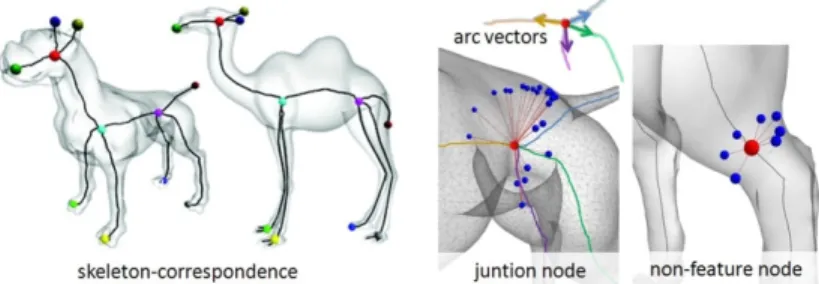
Figure 1: Using the association between the skeletons and

meshes of the objects for shape correspondence. (Left): Skeletal nodes of an object are associated with the local por-tions (marked by the dotted circles) of the mesh of the object; Middle and Right: the mapping between the skeletal nodes of two H-shaped objects O1and O2. If the topological struc-tures of the two skeletons are not considered, the four termi-nal nodes of O1 can be mapped arbitrarily to the terminal

nodes of O2. If geometry properties are not considered, the

skeletal node (1) of O1may be mapped to the skeletal node

(6) of O2.

connects only two feature skeletal nodes. Given a branch b = (n1, n2), we define b/n1:= n2and b/n2:= n1.

A mesh Ω of an object is a pair (VΩ_{, F}Ω_{), where V}Ω_and

FΩare the set of the vertices and the set of the faces, respec-tively. An augmented skeleton K is a triple (V, E, φ), where V is a set of skeletal nodes, E is the set of skeletal arcs connect-ing two adjacent skeletal nodes, and φ is a mappconnect-ing between the vertices of the object and the skeletal nodes. Formally, φ : V → ℘(VΩ), where ℘(VΩ) is the power set of VΩ. The mapping φ defines the association between the skeletal nodes and the vertices.

A measure at a vertex is a scalar function ϕ : VΩ→ R that maps a vertex to a real number. The function ϕ is a kind of surface descriptor at a vertex. For example, the averaged geodesic distance can be measured at a vertex. We define ϕ(n) := _|φ(n)|1 ∑v∈φ(n)ϕ(v), where ϕ(n) is the value

evalu-ated at a skeletal node n and |φ(n)| is the cardinality of the set φ(n).

A skeletal point p lies on a skeletal arc (n1, n2).

Con-sider that the skeletal point is expressed as a linear combi-nation of the two skeletal nodes, i.e. p = αn1+ (1 − α)n2.

To evaluate the value ϕ(p) at a skeletal point p, we have ϕ(p) = αϕ(n1) + (1 − α)ϕ(n2). Here, we focus on linear

in-terpolation for computing the measure in a skeletal point. The other interpolation schemes are possible.

3.2. Algorithm Overview

We exploit the association between the skeletons and meshes of the objects to compute shape correspondence. We com-pute a set of potential correspondences and then select the

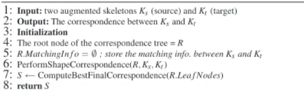
Algorithm 1Augmented Skeleton Correspondence

1:Input:two augmented skeletons Ks(source) and Kt(target) 2:Output:The correspondence between Ksand Kt 3:Initialization

4:The root node of the correspondence tree = R

5:R.MatchingIn f o = ∅ ; store the matching info. between Ksand Kt 6:PerformShapeCorrespondence(R, Ks, Kt)

7:S←ComputeBestFinalCorrespondence(R.Lea f Nodes) 8:return S

best one. Each skeletal node is associated with a set of lo-cal vertices of the mesh. Notice that the vertices mapped to a skeletal node scatter locally on the mesh. The associa-tion roughly represents the mesh properties with the skeletal nodes. Fig.2shows a skeleton of a horse model.

Figure 2: A skeleton and the association between the object

vertices and some skeletal nodes. (a): A skeleton of a horse model. There are skeletal nodes along each skeletal branch. (b): A skeletal junction node (red) and the vertices (blue) associated with it. (c): A skeletal node (red) with degree two and the vertices (blue) associated with it.

The input of our method include two meshes, their skele-tons and some geometric information of the two meshes. We start by matching the core junction nodes and then proceed to match the remaining skeletal branches and skeletal nodes in an interleaving manner. The entire method can be divided into four parts which are Alg.1,2,3and4. Notice that we may merge skeletal nodes during the process (see Alg.2). We describe the details in the following sections.

Algorithm 2PerformShapeCorrespondence(P, Ks, Kt)

1:Input:the node P of correspondence tree; augmented skeletons Ksand Kt 2:matchOneCoreJunctionNodePair(P, Ks, Kt) 3:K0 s←mergeTwoAdjacentJunctionNodes(Ks) 4:if K0 s6= Ksthen 5: add a child C1to P 6: PerformShapeCorrespondence(C1, K0s, Kt) 7:end if 8:K0 t ←mergeTwoAdjacentJunctionNodes(Kt) 9:if K0 t 6= Ktthen 10: add a child C2to P 11: PerformShapeCorrespondence(C₂, Ks, K0 t) 12:end if 13:if K0 s6= Ksand K 0 t 6= Kt then 14: add a child C3to P 15: PerformShapeCorrespondence(C3, Ks0, K 0 t) 16:end if

Our method requires four parameters which are listed in c

2011 The Author(s) c

Online submission ID:1077 / A Skeleton-Based Approach for Shape Correspondence

Algorithm 3matchOneCoreJunctionNodePair(P, Ks, Kt)

1:Input:the node P of correspondence tree; augmented skeletons Ksand Kt 2:foreach node ns∈ Ksdo

3: foreach node nt∈ Ktdo

4: if nscan be matched with ntthen 5: add a child C to P

6: C.MatchingIn f o ← P.MatchingIn f o ∪ (ns, nt) //set matching info. of C. 7: matchRemaining(C, ns, nt, Ks, Kt)

8: end if

9: end for

10:end for

Algorithm 4matchingRemaining(P, ns, nt, Ks, Kt)

1:Input:the node P of correspondence tree;matched junction node pairs (ns, nt); aug-mented skeletons Ksand Kt

2:(B, ˆK1, ˆK2) ← matchBranches(ns, nt, Ks, Kt) 3:if B!= nil then 4: add a child C to P 5: C.MatchingIn f o ← P.MatchingIn f o ∪ B 6: foreach (bs, bt) ∈ B do 7: (n0 s, n 0 t, K 0 s, K 0 t) <- matchJunctionNodePair(C, bs/ns, bt/nt, K 0 s, K 0 t) 8: if(n0 s, n 0 t) != nil then 9: add a child C1to C 10: C1.MatchingIn f o ← C.MatchingIn f o ∪ (n0s, n 0 t) 11: matchRemaining(C1, n0 s, n 0 t, K 0 s, K 0 t) 12: end if 13: end for 14:end if

Table1. The computation is fully automatic once the param-eters are given. In practice, a user can usually obtain accept-able results after tuning the parameters two to three times.

Parameters Purpose Value

K Number of pieces for constructing 8 the branch descriptor (Sec.4.2.2)

λB Clustering of skeletal branches with similar 0.1 branch descriptors (Sec.4.2.2)

CJ Cost for matching skeletal junction nodes 0.012 - 0.025 (Sec.4.2.3)

dJ Distance for merging skeletal junction nodes 5 - 10 (% of the bounding box diagonal of the mesh, Sec.4.2.3)

Table 1: The four parameters of our method.

4. Augmented Skeleton-Based Shape Correspondence

In this section, we present our method for establishing the shape correspondence between two objects by matching their augmented skeletons Ks (source) and Kt (target). We

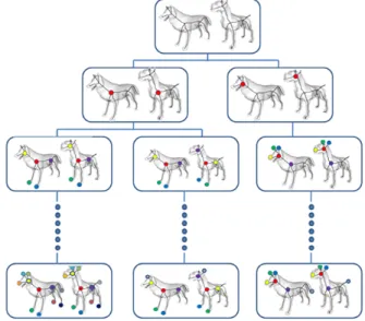
use the subscript s and t to differentiate the elements of the two skeletons. A correspondence tree is built for match-ing the skeletal feature nodes and skeletal branches in a breadth-first-search manner. Each node of the correspon-dence tree stores the matched skeletal feature nodes and skeletal branches while the correspondence tree is built. A schematic diagram of constructing the correspondence tree is shown in Fig.3.

Initially the correspondence tree has one node, i.e. root, which does not contain any matched pairs. Alg.1lists the initialization procedure. We match a skeletal junction node

Figure 3: A correspondence tree for matching two

aug-mented skeletons. Core junction nodes are first matched. The remaining skeletal branches and skeletal junction nodes are matched in an interleaving manner.

pair with the minimum cost and create a node of the corre-spondence tree. The newly created node of the correspon-dence tree becomes the child node of the current inspected node, i.e. the root node. The matching information is stored in the child node. We proceed to match the remaining skele-tal branches and skeleskele-tal nodes in an interleaving manner. This process is invoked recursively until we cannot match any more. Each leaf node of the final correspondence tree represents a correspondence candidate. The leaf node with the minimum cost is the best skeleton correspondence.

4.1. Core Junction Node Correspondence

The centricity cost Ccenter(ns, nt) is defined by:

Ccenter(ns, nt) = |AGD(ns) − AGD(nt)|, (1)

where AGD(·) is the normalized averaged geodesic distance (∈ [0, 1]) of the junction node, which is computed by averaging the AGD values of the ver-tices associated with the junction node. In other words, AGD(ns) = _|φ(n1

s)|∑v∈φ(ns)AGD(v) and

AGD(nt) = _|φ(n1

t)|∑v∈φ(nt)AGD(v). The centricity cost measures how far a skeletal node is away from the center of the object. The definition of the centricity cost is similar to [ATCO∗_{10]. However, we consider the AGD of the}

vertices associated with the skeletal node instead of the skeletal node itself. In this way, the geometric properties of the vertices around the skeletal node can be taken into consideration.

c

2011 The Author(s) c

Online submission ID:1077 / A Skeleton-Based Approach for Shape Correspondence

The structure feature of a junction node is defined by its sub-skeletons. A sub-skeleton of a junction node starts from a skeletal branch attached at the junction node and contains the portion of the skeleton which can be reached by the skeletal branch without getting through the junc-tion node. Fig.4(a) shows the sub-skeletons of a junction node ni. A sub-skeleton can be computed by traversing the

skeleton in a breadth-first-search manner. Assume that ns

has N branches Bs= {s1, s2, ..., sN} and nthas M branches

Bt= {t1,t2, ...,tM}. Denote SG(Bs) = {g1, g2, ..., gN} as a

set of sub-skeletons corresponding to Bs. The normalized

length |g| (∈ [0, 1]) of g is computed as the total length of the skeletal branches of g divided by the total length of all the branches of the skeleton. If there are other branches attached at nsforming the same sub-skeleton, then the sub-skeleton

has a loop(s), as shown in Fig.4(b). The value |g| is then divided by the number of the skeletal branches sharing the same sub-skeleton.

Figure 4: The sub-skeleton of a junction node ni:(a) without

a loop, (b) with a loop.

We define SG(Bt) = {h1, h2, ..., hM} similarly. The

ele-ments of SG(Bs) and SG(Bt) are sorted in decreasing

or-der according to the normalized length of the elements. The structure feature cost Cstruct(Bs, Bt) is defined as

Cstruct(Bs, Bt) = M

∑

∑

Cstructmeasures the similarity of the sub-skeletons generated

at nsandt, respectively. The roles of nsand ntare switched

if N < M. The structure cost is used for measuring the sim-ilarity of the sub-skeletons generated at the junction node pair (ns, nt). The cost Cjunc(ns, nt) for matching (ns, nt) is

defined as

Cjunc(ns, nt) = (Ccenter(ns, nt) + ε) ∗ (Cstruct(Bs, Bt) + ε)

(3) A small positive constant ε is added so that Cjuncis not

com-puted as zero. The value ε is set to 0.01 in our experiments. We match the first junction node pair (ns, nt) with the

min-imum cost Cjunc(ns, nt) and we call this pair the core

junc-tion pair. A core junction node likely locates at the center part of the object. If there are two or more junction node pairs with similar minimum cost, they are also matched

in-dividually and the new nodes of the correspondence tree are created accordingly (see Fig.3).

4.2. Matching Skeletal Branches

We have matched at least one junction node pair (ns, nt) and

then we proceed to match the unmatched branches at (ns, nt).

In this stage, some branches at (ns, nt) may be grouped as

clusters. If this is the case, the new skeleton graphs Ks0and

Kt0 are computed and they are also used for the subsequent

matching process.

4.2.1. Matching Skeletal Branches Using Shape Matching

The local orientation of skeletal branches at a junction node pair (ns, nt) are likely to be similar if the semantics of the

parts around ns and nt are similar. We therefore exploit

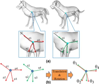
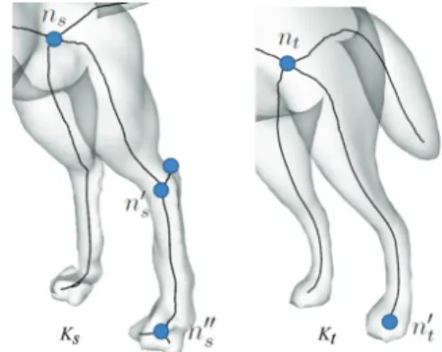
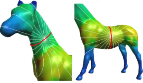
the spatial information for performing skeletal branch corre-spondence. Fig.5shows an example for matching the skele-tal branches of (ns, nt) at the chests of a wolf and a dog.

We compute an inscribed ball centered at the junction node and the radius of the inscribed ball is the average distance between the junction node and its associated vertices. The branch vector is computed based on the portion of the skele-tal branches inside the inscribed ball. The branch vectors are normalized to unit vectors. In the following, we consider only the branch vectors whose corresponding branches are not matched yet.

Figure 5: Skeletal branch correspondence for a junction

node pair. The local orientations of the skeletal branches are similar: (a) compute a branch vector for each skeletal branch; (b) compute the rotation transformation R which minimizes the sum of the distances between the branch vec-tor pairs.

The branch vectors of ns are transformed to the local

c

2011 The Author(s) c

Online submission ID:1077 / A Skeleton-Based Approach for Shape Correspondence

coordinate system at nt such that ns locates at nt (see

Fig. 5(b)). Assume that there are N0 and M0 unmatched skeletal branches at nsand nt, respectively, N0≥ M0. Hence,

there are M0branch pairs to match. In total, there are M0!CN0 M0

combinations for matching the M0_{branch pairs.}

We adopt a greedy approach to match M0 _{branch pairs.}

Assume that P = (p1, p2, ..., pM0) and Q = (q₁, q₂, ..., q_M0),

where pi and qi are the unit branch vectors at the

matched junction pair (ns, nt). We employ shape matching

[MHTG05] to compute a rotation matrix R by minimizing the sum of the distances between the branch vector pairs. The angle difference between a branch vector pair (pi, qi) is:

ang(pi, qi) = acos(dot(pi, Rqi))/π, (4)

where dot(·, ·) is the dot product of two vectors. The spatial cost for (P, Q) is given by

Cspatial(P, Q) = M0

∑

i=1

(ang(pi, qi))2. (5)

Now, the cost for matching P and Q is computed as

Cbranch(P, Q) = (Cstruct(Bs(ns), Bt(nt))+ε)∗(Cspatial(P, Q)+ε).

(6) The cost Cbranchnot only depends on the spatial

orienta-tion of the skeletal branches but also the structures of the sub-skeletons generated at nsand nt. We sort all the

possi-ble skeletal branch correspondences with ascending cost and select the first 10% of the skeletal branch correspondences. For each possible branch correspondence (P, Q) at (ns, nt),

a new node of the correspondence tree is created. After that we have matched the M0_{skeletal branch pairs. The roles of}

Pand Q are swapped if M0> N0.

The rotation matrix R can be used for filtering the bad skeletal branch correspondences which are due to symmetry. If the determinant of the R is negative (i.e. -1), it represents that the rotation matrix involves a reflection. Such a skeletal branch correspondence should be ignored.

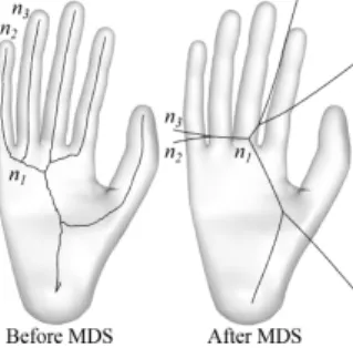
We do not adopt MDS [EK03] for computing the branch vectors. This is because the relative orientations of some branches may not be maintained, as shown in Fig.6.

4.2.2. Clustering of Skeletal Branches

Some parts of a mesh have the same semantic meanings, such as front/back legs and ears. They have similar shapes and geometric features. We can group these similar parts as clusters in order to prune bad correspondences. The idea is as follows. Each part is usually associated with a skele-tal branch. We divide each skeleskele-tal branch b into K pieces, namely b1, b2, ..., and bK. After that we can compute a

value for the geometric property of each piece. In our case, we compute MSP value of each piece (see MSP value in Sec.5). MSP value captures roughly the local volume around a skeletal node. The advantage of using MSP value over the

Figure 6: The two skeletons are obtained before and after

applying MDS, respectively. The two branches(n1, n2) and

(n1, n3) are symmetric with respect to the junction node n1

after MDS is performed.

radius of the maximum sphere at a skeletal node is that us-ing MSP value is more suitable if the objects deform. Con-sider a deformed circle in Fig. 8. The radius of the cir-cle changes significantly but its perimeter does not change much. We have MSP(bk) =

R

p∈bkMSP(p)d p

|bk| , where |bk| is the length of bk. The value MSP(bk) is normalized by the

max-imum MSP value of individual objects so that MSP(bk) is

scale-invariant. There are K values for each branch and they are assembled as a k-dimension vector, namely, branch de-scriptor. Assume that there are two branch descriptors `iand

`j. The corresponding two skeletal branches are clustered if

k`i− `jk2≤ λB. The branch clusters are illustrated in Fig.7.

If two branches are clustered, they cannot be clustered with other branches. To handle three or more branches with sim-ilar branch descriptors, we create a new node of the corre-spondence tree for each pair of the branches.

Figure 7: Clusters of the skeletal branches at a junction

node ni. Each cluster is drawn in the same color. Left: The

two back legs; Middle: The two front legs; Right: The two two ears.

Figure 8: A deformed circle. Its perimeter does not change

much but the radius of the maximum incircle is changed sig-nificantly.

c

2011 The Author(s) c

Online submission ID:1077 / A Skeleton-Based Approach for Shape Correspondence

The skeletal branch clusters can be used for eliminating most of the bad correspondences for skeletal branches. Con-sider the case in Fig.5in which the front legs of the wolf and the dog are clustered, respectively. These two clusters are matched and then the skeletal branches associated with the necks and trucks are matched. We do not match the clustered skeletal branches with the non-clustered skeletal branches. The number of branch pairs for checking is reduced from 4!=24 to 2!2! = 4, in this case.

4.2.3. Matching Junction Nodes

To determine whether or not a junction node n0sshould be

matched with a junction node n0

t, we compute the cost for

matching (n0s, n0t) using Equation3. If the cost is smaller than

or equal to a threshold CJ, they are matched. If not, we adopt

junction node merging or branch merging to find the other closest junction nodes for matching.

Junction node mergingcan be employed for merging the

adjacent junction nodes if the distance between the junction nodes is less than or equal to dJ. Consider the case for

match-ing n0swith n0t, as shown in Fig.9. But n0scannot be matched

with n0

t due to the topological difference and Cjunc(n0s, n0t)

is too high. After n0s and n0t are merged with their adjacent

junction nodes, they can be matched. Notice that junction node merging is also applied when the core junction pairs are computed. Branch merging is performed if junction node merging does not work.

Figure 9: Matching n0s with n0t using junction node

merg-ing. The two nodes n0sand n0t(colored red) are matched after

merging them with the adjacent junction nodes (inside the two red dotted circles).

Branch mergingis adopted to match non-adjacent

junc-tion nodes. Consider the case that the juncjunc-tion node pair (ns, nt) has been matched. We want to match the next

junc-tion node pair from the two sub-skeletons of (ns, nt). We

check the closest junction node pair (n0

s, nt0) but find out that

they cannot be matched. This is because an unwanted short branch is attached at n0

sand the cost is too high for

match-ing. To solve this problem, we find the other junction node from the sub-skeletons generated by either n0

sor n0t. The

pro-cess is repeated until a junction node pair can be matched

or no more can be matched. Fig.10shows an example in which the two branch paths (ns, n00s) and (nt, n0t) are checked

for matching. In this case, the two source branches (ns, n0s)

and (n0s, n00s) are merged into a new branch (ns, n00s). Hence,

we successfully match n00

s with n0t.

If branch merging or junction node merging is performed, the new skeleton graphs Ks0 and Kt0are computed and they

are used for the subsequent matching process. After we have matched a junction node pair, we proceed to match the re-maining unmatched branches.

Figure 10: Matching (ns, n00s) with (nt, n0t) using branch

merging. The cost of matching n0s with nt0 is too high due

to the local topological difference. After performing branch merging, i.e. merging branches (ns, n0s) and (n0s, n00s) into

(ns, n00s), n00s can be matched with n0t.

4.3. Final Skeleton Correspondence

Each leaf node of the final correspondence tree represents a candidate correspondence. The maximum costs of Cjunc

and Cbranchare computed and they are used for normalizing

each cost to (0, 1]. The sets of costs Cjuncand Cbranchof a

leaf node are denoted as {c₁j, c₂j, ..., c_Nj j} and {c

b

1, cb2, ..., cbNb}. Then the cost of a leaf node is given by:

Clea f= Π Nj i=1c j i∗ Π Nb i=1c b i (7)

Usually, the cost of a leaf node is smaller if there are more matched skeletal node and branch pairs. The leaf node with the minimum cost is selected as the best correspondence.

5. Implementation

We adopt the minimum slice perimeter (MSP) [HJWC09] for computing our skeletons in the preprocessing stage. MSP of a vertex captures the local volume of the vertex. The method by [ATC∗_{08] can also be adopted. Once the}

skele-tons are constructed, the mapping φ between the vertices and the skeletal nodes is obtained intrinsically. We briefly review the MSP function and then the MSP skeleton as follows. c

2011 The Author(s) c

Online submission ID:1077 / A Skeleton-Based Approach for Shape Correspondence

The MSP function is a scalar function defined on the sur-face of a mesh. Slices of a point p are defined as the inter-section curves with the set of planes generated by the nor-mal of the surface in p. The MSP value of p is the minimum perimeter of all slices of p. The MSP value of a point is usu-ally approximated by uniformly sampling as it is not easy to generate all the slices of the point. In our experiments, we used 12 slices for each point. An example is shown in Fig.11

for computing the MSP value of a point. The MSP value of a point can be used for approximating the volume around a slice by supplying a thickness value.

Figure 11: The MSP value of a point p (red thick line). There

are 12 slices for each model.

An MSP skeleton is built as follows. The slice of each vertex which has the minimum perimeter is computed. Each vertex is then transformed to the center point of the inter-sected curve between the minimum slice and the object. The transformed vertices likely locate at the interior of the origi-nal mesh and they form a new mesh which is skinny. We call this skinny mesh a shrunk mesh. A greedy skeletonization process is then employed for degenerating the shrunk mesh by performing a sequence of edge swap operators in order to obtain a 1D curved skeleton. The greedy skeletonization pro-cess is similar to [ATC∗_{08]. During the process, the}

trans-formed vertices are merged to obtain skeletal nodes. Hence, each skeletal node of the curved skeleton is mapped to a set of the vertices. Some of the vertices may not be associ-ated with any skeletal nodes because unwanted short skeletal branches and their corresponding vertices are removed.

6. Results and experiments

We present the results of our method for computing shape correspondence and then discuss its limitations.

Results. In the preprocessing stage, we computed the

skeletons of the models and AGD of the vertices. We then applied our method for a variety of models. The dog skele-ton is the source. The skeleskele-ton correspondence results are shown in Fig.12. The matched node pairs are drawn in the same colors but the unmatched nodes are not shown. All of the semantic parts (e.g. legs, heads, and ears) are matched correctly. Since our method performs junction node merging and branch merging, there may be one-to-many or many-to-many correspondences between junction nodes and also

between branches. This is different from the previous ap-proaches [HSKK01,BMSF06,ATCO∗10] which establish only one-to-one mapping. For example, a junction node at the chest of the dog is matched with two junction nodes at the chest of the goat. Our method can handle the skeletons of chairs with loops, as shown in Fig.13.

Comparisons.We compared our method with the method

by Au et al. [ATCO∗10]. Fig.14shows two sets of corre-spondence results. For the top example, their method mis-matches an ear of the horse to the jaw of the dog. For the bottom example, their method mismatches the ears of the pig to the upper jaw of the dragon. Our method produces correct results due to branch clustering. The ears form clusters and they cannot be matched with the non-clustered jaws.

Compared to [BL08], our method can match the internal nodes of the skeletons. Our method matches the core tion nodes, and then match the remaining branches and junc-tion nodes in an interleaving manner. So that our method can match the internal nodes.

Model #Tri. AGD MSP SE MAS Function Function Dog(source) 18976 157.71 25.86 33.23 -Deer 7402 22.23 5.04 3.57 0.20 Human 11258 43.05 5.10 9.74 0.22 Armadillo 20000 193.32 30.10 23.63 0.24 Dragon 16000 199.02 27.79 28.16 0.19 Triceratops 15764 104.33 18.17 27.44 0.21 Elephant 30000 500.30 52.73 146.08 0.30 Asian dragon 28198 490.70 44.54 37.28 0.41

Table 2: Model complexities, the timings (sec) of the

pre-processing tasks and the timings of matching the augmented skeletons. SE: Skeleton extraction; MAS: Matching the aug-mented skeletons.

Timing information.All the results were performed on

Intel Core 2 Duo CPU E8400 3.0GHz with 4GB memory, us-ing a sus-ingle thread implementation. We precomputed AGD function, MSP function, and skeleton extraction. Table 2

shows the timing information of the preprocessing computa-tion and the timings of performing the shape correspondence (i.e. matching the augmented skeletons of the objects). The computation time for shape correspondence is under 0.5 sec-ond in all our experiments. Table3shows the information of the correspondence trees which were constructed for match-ing the augmented skeletons of the objects.

The searching space of our method is smaller than the combinatorial searching method [ZSCO∗_08,ATCO∗_{10] as}

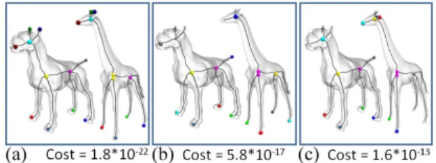
we perform branch clustering. The total number of the pos-sible matchings between the two skeletons reduce dramati-cally. Fig.15shows three leaf nodes of the correspondence tree for matching the skeletons of the dog and giraffe mod-els. The best result is shown in Fig. 15(a). The cost of the best node is smaller if more feature nodes and skeletal branches are matched. Similar to other existing techniques, our method requires the manual operations to change the pa-rameters if the results are not good. It usually takes a few

c

2011 The Author(s) c

Online submission ID:1077 / A Skeleton-Based Approach for Shape Correspondence

Figure 12: Shape correspondence results between a dog and a variety of models: goat, camel, deer, giraffe, cat, pig, human,

armadillo, dinosaur, triceratops and Asian dragon. The matched node pairs are drawn in the same colors.

Figure 13: Shape correspondence results for ant, teddy and chair models.

minutes for making several attempts to obtain the desired results.

Model #Tree Tree #Core #Branch #Branch #Leaf Nodes Height Junction and Node Clusters Nodes

Nodes Merging Dog(source) - - - - -Goat 18 4 3 12 20 4 Deer 18 4 3 15 26 5 Giraffe 23 4 3 8 36 7 Cat 18 4 3 8 22 5 Pig 11 4 3 0 16 3 Human 12 3 2 4 16 4 Armadillo 18 4 3 0 24 5 Dragon 14 4 3 0 18 4 Ant 42 5 4 50 24 10 Teddy 13 4 3 0 24 4 Chair 6 6 5 0 2 1

Table 3: Information of the correspondence trees.

Discussions and limitations.Our method may mismatch

the branch clusters (e.g. mapping the ears of the horse to the horns of the cows) because of a lack of the semantic knowl-edge. In addition, some objects having flat shape around the junction nodes may not be inferred the front or back side by skeletons. A flipping correspondence may be obtained.

Figure 15: Some leaf nodes of the correspondence tree of

matching the skeletons of the dog and giraffe models. (a): Best result; (b): the chest of the dog is matched with the belly of the giraffe; (c): the head of the dog is matched with the mouth of the giraffe.

Our method requires manual operations to set the parame-ters and it may take several attempts to obtain acceptable re-sults. Finally, we cannot construct good skeletons for some man-made models (e.g., cups, sphere ball, or engineering models) and the quality of shape correspondence results is affected. If the skeletons do not capture the shape of the meshes faithfully, our method may not work properly. c

2011 The Author(s) c

Online submission ID:1077 / A Skeleton-Based Approach for Shape Correspondence

Figure 14: Comparison with the method [ATCO∗10]. Left: the results of [ATCO∗10]; Right: our results. Their method

mis-matches the nodes at the heads (highlighted by the red squares).

7. Conclusions

We have presented a novel skeleton-based approach for com-puting shape correspondence. Our method may merge skele-tal nodes and branches so that it may compute 1-1 corre-spondences and many-many correcorre-spondences. Our method has been tested for a variety of similar objects and they may have different poses. The experimental results show that our method can compute acceptable shape correspondence.

Our method relies on the association between the skeletal nodes and object vertices, but we do not consider the actual shape of the parts for matching. Our method may fail to com-pute a reasonable shape correspondence if the objects are not similar. One possible extension of our work is to consider the actual shape of the parts so that partial correspondence can be computed. Another possible extension is that instead of selecting the core junction nodes, the parts of the objects are first extracted by employing skeletons. After that we can match the parts and build the entire shape correspondence. Furthermore, we would like to apply prior knowledge with our method for computing shape correspondence.

References

[ATC∗_{08] AUO. K.-C., TAIC.-L., CHUH.-K., COHEN-OR} D., LEET.-Y.: Skeleton extraction by mesh contraction. ACM

TOG 27, 3 (2008).

[ATCO∗_{10] AUO.-C., TAIC., COHEN-ORD., ZHENGY., FU.} H.: Electors voting for fast automatic shape correspondence.

Comp. Graph. Forum 29, 2 (2010), 645–654.

[BL08] BAIX., LATECKI L.: Path similarity skeleton graph matching. IEEE Trans. on PAMI 30 (2008), 1282–1292.

[BMSF06] BIASOTTIS., MARINIS., SPAGNUOLOM., FALCI

-DIENOB.: Sub-part correspondence by structural descriptors of 3D shapes. Comp. Aided Design 38, 9 (2006), 1002–1019. [EK03] ELADA., KIMMELR.: On bending invariant signatures

for surfaces. IEEE Trans. on PAMI 25 (2003), 1285–1295. [HJWC09] HOT. C., JIH. X., WONGS. K., CHUANGJ. H.:

Mesh skeletonization using minimum slice perimeter function.

Computer Science Technical Report CS-TR-2010-0001, The Na-tional Chiao Tung University, Taiwan, R.O.C.(2009).

[HSKK01] HILAGAM., SHINAGAWAY., KOHMURAT., KUNII

T. L.: Topology matching for fully automatic similarity estima-tion of 3D shapes. In SIGGRAPH (2001), pp. 203–212. [MHTG05] MÜLLERM., HEIDELBERGERB., TESCHNERM.,

GROSSM.: Meshless deformations based on shape matching.

ACM TOG 24, 3 (2005), 471–478.

[MS01] MORTARAM., SPAGNUOLOM.: Similarity measures for blending polygonal shapes. Computers and Graphics 25, 1 (2001), 13–27.

[SSGD03] SUNDARH., SILVERD., GAGVANIN., DICKINSON

S.: Skeleton based shape matching and retrieval. In Shape

Mod-eling Int’l(2003), p. 130.

[TS04] TUNG T., SCHMITT F.: Augmented reeb graphs for content-based retrieval of 3D mesh models. In Shape Modeling

Int’l(2004), pp. 157–166.

[vKZHCO10] VAN KAICK O., ZHANG H., HAMARNEH G., COHEN-ORD.: A survey on shape correspondence.

Eurograph-ics State-of-the-art Report(2010).

[ZSCO∗_{08] ZHANGH., SHEFFER A., COHEN-OR D., ZHOU} Q.,VANKAICKO., TAGLIASACCHIA.: Deformation-driven shape correspondence. Symposium on Geometry Processing

(2008), 1431–1439.

c

2011 The Author(s) c

SAI-KEUNG WONG, JAU-AN YANG, TAN-CHI HO AND JUNG-HONG CHUANG

A Skeleton-Based Approach for

Consistent Segmentation Transfer

SAI-KEUNG WONG, JAU-AN YANG, TAN-CHI HO, JUNG-HONG CHUANG Department of Computer Science

National Chiao Tung University Hsin-chu, 300 Taiwan

We present a skeleton-based approach for mapping consistently a segmentation of a source mesh to a target mesh. The source and target meshes are semantically similar but their geometries may be different. We assume that the segmentation of the source mesh and the skeleton correspondence between the meshes are provided. Our method first establishes the skeleton-boundary correspondence and then performs the boundary transfer procedure. The skeleton-boundary correspondence is useful for computing approximately the target boundaries. The boundary transfer procedure aims to produce the segment boundaries of the target mesh such that their geometric details are consistent to the ones of the corresponding source segment boundaries. We have applied our method for various models and compared with the state-of-the-art techniques. Our method computes segment boundaries of the target mesh which are similar to the ones of the source mesh.

Keywords: segmentation transfer ···· skeleton correspondence ···· consistent segmentation···· geometric algorithms ····

skeleton-boundary correspondence

1. INTRODUCTION

Mesh segmentation refers to partitioning a mesh into meaningful disjoint sub-patches or parts. It is a fundamental technique in computer graphics. Much effort has been devoted for segmenting individual objects into parts. Segmenting a set of similar objects consistently is required in applications, such as object retrieval and object classification [10].

Skeleton is an important object descriptor which encapsulates the structure of an object [4]. The skeleton correspondence between two objects establishes the matching for their similar semantic parts. Similar objects are likely to be segmented similarly for the matched parts as the similar semantic parts of the objects are likely to be segmented consistently. In this paper, we develop a skeleton-based approach for mesh segmentation transfer which can be applied to compute consistent segmentation for a set of similar objects. Given the segmentation of the source mesh and the skeleton correspondence between the source and target meshes, our method transfers the segment boundaries of the source mesh to the target mesh. Our method requires the skeleton-mesh correspondence which is useful for computing consistent segmentation.

In skeleton-mesh correspondence, each skeletal node corresponds to a set of mesh vertices and a skeletal arc consists of a set of skeletal nodes. Consider that we have a segmented mesh and its skeleton. Notice that a segment boundary consists of a set of vertices. Hence, the mapping between the skeletal nodes and the mesh vertices can be used for establishing the mapping between the skeletal nodes and the segment boundaries. Furthermore, the source segment boundaries can then be transferred approximately to the target mesh according to the skeleton correspondence. Finally, we refine the segment boundaries of the target mesh so that they are similar to the corresponding source segment boundaries. We have evaluated our method for various models and compared with the state-of-the-art techniques. Experimental results show that our method computes acceptable segmentation of the target meshes.

2. RELATED WORK

We review mesh segmentation techniques which are mostly related to our method. Mesh segmentation has been researched extensively [27,16,1,20,15,19,26,18,28,10,31]. Some mesh segmentation algorithms