基於決策樹學習的變數相依性測定法

(1)

國

立

交

通

大

學

資訊科學與工程研究所

碩

士

論

文

基於決策樹學習的變數相依性測定法

Linkage Identification Based on Decision Tree Learning

研究生：黃淵暐

指導教授：陳穎平教授

中

華

民

國

九

十

九

年

六

月

(2)

基於決策樹學習的變數相依性測定法

Linkage Identification Based on Decision Tree Learning

研究生：黃淵暐 Student：Yuan-wei Huang

指導教授：陳穎平 Advisor：Ying-ping Chen

國立交通大學

資訊科學與工程研究所

碩士論文

A Thesis

Submitted to Institute of Computer Science and Engineering College of Computer Science

National Chiao Tung University in partial Fulfillment of the Requirements

for the Degree of Master

in

Computer Science

June 2010

Hsinchu, Taiwan, Republic of China

(3)

基於決策數學習的變數相依性測定法

Linkage Identification Based on Decision Tree Learning

學生：黃淵暐

指導教授：陳穎平教授

國立交通大學資訊科學與工程研究所

摘

要

基因演算法及衍生的演算法在過去的研究與應用裡，已展現了其廣泛而有效率、且具備實用性的特性。為了進一步增進基因演算法的能力，各式的方法在演化式計算的研究領域裡被提出；其中一主要的方向在於找出問題中各項變數彼此間的相依性、藉改善其內部預算子的效率以達到增進整體效率的目的，如 Estimation of Distribution Algorithms、Perturbation-based Methods。

本研究嘗試探討 Inductive Linkage Identification 和各種不同的決策樹學習演算法搭配下的特性、觀察其在不同實驗設定下展現的效能差異；實驗除了包含了 4 級(order-4)與 5 級(order-5)的環形問題結構，也包括了高基數(high cardinality)變數的實驗探討。實驗結果顯示出在二元(binary)變數的問題裡，各種決策樹學習演散法對類似的問題結構，需要著相同時間複雜度來正確鑑定出其結構；而對於高基數的問題，搭配不同的決策數學習演算法會需要不同的運算資源。關關關關鍵鍵鍵鍵字字字字：：：：演化計算、基因演算法、變數相依性學習、問題結構、建構模塊

(4)

Abstract

Genetic algorithms and their descendant methods have been deemed robust, effective, and practical for the past decades. In order to enhance the features and capabilities of genetic algorithms, tremendous effort has been invested within the research community of evolutionary computation. One of the major development trends to improve genetic algorithms is trying to extract and exploit the relationship among decision variables, such as estimation of distribution algorithms and perturbation-based methods. In this study, we attempt to investigate the integration of perturbation-based method, inductive linkage identification (ILI), and decision tree learning algorithms for detecting general problem structures. Experiments on circular problems structures composed of order-4 and order-5 trap functions are conducted, as well as the experiments on the cardinality of variables. Our experiments results indicates that this approach requires a population size growing logarithmically and is insensitive to the problem structure consisting of similar sub-structures as long as the overall problem size is identical and those variables are binary. Experiments also shows that different adopted decision tree learning algorithms will demand different requirements when the variables are extended to higher cardinalities.

keywords:

Problem structure, inductive linkage identification, ILI, linkage learning, problem decom-position, overlapping building block, non-overlapping building block, perturbation-based method, genetic algorithm, evolutionary computation

(5)

List of Figures

3.1 Graph-like presentations of interactions among variables. . . 9

4.1 The decision tree learned from Table 4.1. . . 13

4.2 Problem structures detected during the linkage detection process. Dashed and solid lines represent known and newly discovered interactions respectively. 14 4.3 Decision tree constructed by different learning algorithms. . . 15

4.4 Comparison between the entropy and the Gini index. . . 18

4.5 The example of the third constraint of the impurity function. . . 18

5.1 Circular problem structures used in experiments. . . 20

5.2 Required population sizes against increasing problem sizes. . . 22

5.3 Functions used as the subproblems in section 5.2. . . 23

5.4 Required population sizes for different composing subproblems. . . 23

5.5 Circular problem structures composed of separate sub-structures, where n = 5. . . 24

5.6 Circular problem structures composed of one, two, and three sub-structures with trap4 as the elementary sub-problems. . . 25

(8)

List of Tables

(9)

Chapter 1 Introduction

As practical optimization frameworks, genetic algorithms (GAs) have shown properties of flexibility, robustness, and ease-of-use since they were proposed [1, 2]. During the op-timizing procedures, candidates of problem solution are encoded into designed genotype presentations and good candidates are selected to exchange information via genetic oper-ations like crossover and mutation. Thus better solutions are probably produced in the next generations. Since the information exchanging is essential component in the frame-works, carefully designed mechanisms might increase the efficiency of the optimization process.

1.1 Motivation and Objective

Crossover operators in early genetic algorithms are likely to break promising solutions of sub-problems, which are referred to as building blocks (BBs) [3]. As a consequence, the overall performance is greatly reduced, or the problem cannot be solved [4]. In or-der to alleviate this issue, in recent studies, crossover operators or equivalent mecha-nisms that maintain the structure and diversity of building blocks have been proposed, developed, and examined [5]. These techniques significantly increase the performance of genetic algorithms. To provide the capability of appropriately and effectively han-dling sub-solutions/building blocks, two key mechanisms, building-block identification and building-block exchange, have to be utilized and integrated in the GA framework. In this study, we focus on the mechanism of building-block identification, generalize the concept regarding the detection of building blocks.

(10)

Based on inductive linkage identification [6], a modification approach is proposed to detect general problem structure. This approach investigate the concept of using decision tree learning as a tool for linkage identification. Two adoptions of this approach are experimented on several issues to verify their capabilities, including the problem size, the inner problem structure, the composing sub-functions, and the cardinality of variables.

1.2 Road Map

For the reminder of this thesis, previous researches on this topic are briefly reviewed in the next chapter. The background of linkage identification is introduced in chapter 3. Chapter 4 describes why and how the proposed approach works with an illustrated ex-ample. Experiments examining different issues are provided in chapter 5 and discussed in chapter 6. Followed by a final chapter to summery and to conclude this research.

(11)

Chapter 2 Reviews of Linkage Identification

As mentioned in the chapter 1.1, the performance of GA optimizations can be improved while the adopted genetic operators maintain those dependencies among variables well. However, foreknowledges are required to design such operators, which is usually not the case when GAs are applied. Devoting to obtaining those informations, numbers of ap-proaches have been proposed. According to the aspects those researches consider the linkage identification problem with, mechanisms can be roughly classified into three cat-egories [7]: (1) Linkage Learning, (2) Estimation of Distribution Algorithms, and (3) Perturbation Methods.

2.1 Linkage Learning

Approaches in this category view building-block identification as the (gene/variable) or-dering problem. By rearranging variables during the evolutionary process, interdependent variables are put closer according to the adopted coding scheme such that these variables are less likely to be split apart by subsequent operations. In these studies, the messy genetic algorithm [4] and its more efficient descent, the fast messy genetic algorithm [8], exploit building blocks to identify linkages.

Since the rearranging mechanism often acts too slow to cooperate with the selection operator, such a condition usually leads to the premature convergence. The linkage learn-ing genetic algorithm [9] performs two-point crossover on a specifically designed circular chromosome representation such that tight linkages among related variables can be formed on the chromosome and preserved during the evolutionary process.

(12)

2.2 Estimation of Distribution Algorithms

The statistic view of points leads to Estimation of Distribution algorithms (EDAs) [10, 11, 12]. These approaches describe the dependencies among variables in a probabilistic manner by constructing a probabilistic model from selected solutions and then sample the built model to generate new solutions. Early EDAs began with assuming no interac-tions among variables, such as the population-based incremental learning (PBIL) [13] and the compact genetic algorithm (cGA) [14]. Subsequent studies started to model pairwise interactions, e.g., the mutual-information input clustering (MIMIC) [15], Baluja’s depen-dency tree approach [16], and the bivariate marginal distribution algorithm (BMDA) [17]. Multivariate dependencies were then exploited and more general interactions were mod-eled. Example methods include the extended compact genetic algorithm (ECGA) [18], the Bayesian optimization algorithm (BOA) [19], the factorized distribution algorithm (FDA) [20], and the learning version of FDA (LFDA) [21]. Despite of building multivari-ate probabilistic models directly from the population, ϕ-PBIL [22] clusters the population into several groups according to the similarity of solutions and analyzes the probabilistic distributions of groups produced by PBIL to capture interactions among variables.

Since model constructing in these methods requires no additional fitness evaluations, EDAs are usually considered efficient in the traditional viewpoints of evolutionary compu-tation, especially when fitness evaluations involve time-consuming simulations. However, the model constructing mechanism itself is sometimes computationally expensive with the large populations size, which repeatedly occurs in evolutionary methods. The difficulty which EDAs often face is that those building blocks contributing less to the total fitness are likely ignored rather than captured.

2.3 Perturbation Methods

Since variables of the same building block determine the fitness contribution simultane-ously while other variables do not, perturbation, i.e., change the value of a given variable, can be a tool to detect the dependencies on a given variable. In the literature, the gene expression messy GA (GEMGA) [23] represents the sets of tightly linked variables as

(13)

weight values assigned to solutions and employs a perturbation method to detect them. GEMGA observes the fitness changes caused by perturbation on every variable for strings in the population and detects interactions among variables according to how likely those variables compose the optimal solution. Assuming that nonlinearity exists within a build-ing block, the linkage identification by nonlinearity check (LINC) [24] perturbs a pair of variables and observes the presence of nonlinearities to identify linkages. If the sum of fitness differences of perspective perturbations on two variables equal to the fitness differ-ence caused by simultaneously perturbing the two variables, the linearity is determined and thus, these two variables are considered independent. Instead of the non-linearity, the descendant of LINC, linkage identification by non-monotonicity detection (LIMD) [7], adopts non-monotonicity to detect interaction among variables.

Compared to EDAs, the low salience building blocks are unlikely ignored in these approaches. However, since obtaining fitness differences requires extra function evalua-tions, perturbation methods are usually regarded demanding more computational efforts to detect linkages. In addition to empirical studies, Heckendorn and Wright generalized these methods through a Walsh analysis [25] to obtain theoretical resource requirements. Zhou et al. later extended this study from the binary domain to high-cardinality do-mains [26, 27].

An interesting algorithm combining the ideas of EDAs and perturbation methods,

called the dependency detection for distribution derived from fitness differences (D5_{), was}

developed by Tsuji et al. [28]. D5 _{detects the dependencies of variables by estimating the}

distributions of strings clustered according to fitness differences. For each variable, D5

calculates fitness differences by perturbations on that variable for the entire population and clusters the strings into sub-populations according to the obtained fitness differences. The sub-populations are examined to find k variables with the lowest entropies, where

k is the algorithmic parameter for problem complexity (the number of variables in a

linkage set). The determined k variables are considered forming a linkage set. D5 _can

detect dependencies for a class of functions that are difficult for EDAs (e.g., functions containing low salience building blocks) and requires less computational cost than other perturbation methods do. However, its major constraint is that it relies on an input

(14)

parameter k, which may not be available due to the limited information to the problem

structure. As a side-effect to the parameter k, D5 _{might be fragile in the situation where}

(15)

Chapter 3 Linkages, Building Blocks, and

Problem Structures

In this chapter, we first review the definitions and terminologies which will be used through out this thesis, and then describe the generalized concept of “problem structure” derived from “building block.”

3.1 Dependencies among Variables

De Jong et al. [29] defined the term dependency, which is also referred to as linkage, as “two variables in a problem are interdependent if the fitness contribution or optimal setting for one variable depends on the setting of the other variable.” Moreover, the

order of a problem is also stated as “the order is the largest number of variables that

are interdependent.” To obtain the complete information of linkages, the contribution of each possible pair of variables needs to be examined. Although it is usually an expensive work to process all possible pairs of variables, dependencies should be examined as much as possible in a reasonable time such that the employed genetic algorithm can perform well.

The Schema theorem [1] states that short, low-order, and highly fit sub-solutions in-crease their market shares to be combined. Furthermore, the building block hypothesis [3] implies that combining small partial solutions is essential for genetic algorithms and also consistent with human innovation.

According to these observations, a problem model called the additive decomposable

(16)

identi-fication.

3.2 Additive Decomposable Function

This problem model is written as the sum of low-order sub-functions, a.k.a., sub-problems.

Let a string of length `, s = s1s2s3. . . s`, present a solution, where s is a permutation of

the decision variables x = x1x2x3. . . x` determined by the adopted coding scheme. The

fitness function for s is then defined as

f (s) =

m

X

i=1

fi(svi) ,

where m is the number of sub-functions, fi(·) is the i-th sub-function, and svi is the

solution string for fi(·). For example, if vi = (4, 2, 3, 6), svi = s4s2s3s6. If fi(·) is also a

sum of other sub-functions, it can be replaced by these sub-functions. Therefore, without

loss of generality, each fi(·) can be assumed a non-linear function, and the number of

variables of fi(·) is referred to as its order, i.e., complexity.

In the ADF model, the ordering property is eliminated and thus those variables in the

same set viare interdependent. These sets referred to as linkage sets, and the related term

building block (BB) is used for the candidate solutions to the corresponding sub-functions.

3.3 Problem Structure

For complex problems, those composing sub-problems might be overlapping likely. Similar to interdependent variables, shared variables affect the respective contributions of the overlapping building blocks to the total fitness of the problem and make these building blocks interdependent. Different linkage identification mechanisms might detect those overlapping sub-problems as either separated, shorter linkage sets or a single, longer one. As a tool acquiring information of interdependency among variables for optimizations, these two approaches acts as complementary roles: the former provides preciser and more detailed information, and the later gives the overall interactions which should be considered in the sub-function level as well as in the variable level.

Reviewing previous studies on pairwise interactions, building blocks, and order-k link-age sets, researchers attempt to capture structures of certain complexities. However, if

(17)

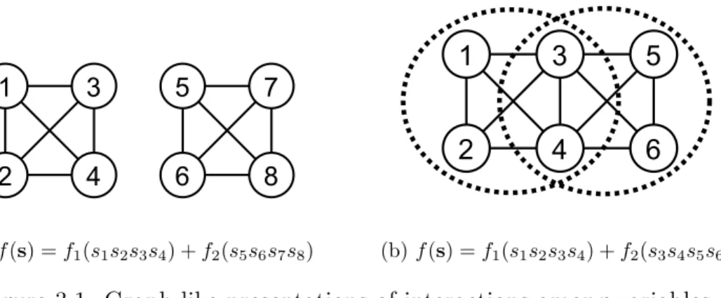
(a) f (s) = f1(s1s2s3s4) + f2(s5s6s7s8) (b) f (s) = f1(s1s2s3s4) + f2(s3s4s5s6)

Figure 3.1: Graph-like presentations of interactions among variables.

the overall structure can somehow be recognized as that obtained by the model build-ing process in estimation of distribution algorithms, perturbation-based methods should also be able to provide sufficient understandings of the problem for those linkage-aware operations.

Therefore, in this thesis, we generalize the concept of overlapping building blocks to the notion of the problem structure such that interactions among variables can be described as general as possible. Figure 3.1 illustrates the dependencies among variables: Figure 3.1(a) presents 2 separate oreder-4 functions while Figure 3.1(b) are 2 overlapped order-4 functions(denoted by the dotted circles). The term sub-problem is used to describe how the overall problem structure is constructed instead of decomposed. The terms

(18)

Chapter 4 Proposed Approach

In the researches [6, 30], the Inductive Linkage Identification (ILI) was proposed with the efficient performance against the increasing problem size and the sub-function complexity on the non-overlapping problem composition. Based on these researches, a more general and flexible approach is introduced.

4.1 Fitness Difference Values and Decision Tree

Learn-ing

In this section, the concept of adopting decision tree learning is described with examples. Firstly, observe the exemplary problem following the ADF model and the fitness difference

df1 derived from perturbed variable s1:

f (s1s2s3. . . s8) = subf unction3(s1s2s3) + subf unction5(s4s5s6s7s8) . (4.1)

df1 = f (s1s2s3. . . s8) − f (s1s2s3. . . s8)

= (subf unction3(s1s2s3) + subf unction5(s4s5s6s7s8))

−(subf unction3(s1s2s3) + subf unction5(s4s5s6s7s8))

= subf unction3(s1s2s3) − subf unction3(s1s2s3) .

(4.2)

Equation 4.2 suggests that the fitness difference value is only determined by those sub-functions where the perturbed variable belongs. Be more specific, since the fitness contributions from other sub-functions are eliminated after the subtraction, a certain permutation of values of those remaining variables will cause a certain fitness difference value. Giving a population which is large sufficiently, those patterns between variables

(19)

and fitness differences should occur lots of times and be captured by any well-developed mechanisms. Once those patterns are identified, variables involved in patterns are con-sidered interdependent as a linkage set. Furthermore, this derivation is conducted only under the ADF assumption, therefore extended to the most generalized form with any kind of subproblems and variable domains.

In the field of Machine Learning, a well-studied topic appears as the following: giving a set of statements composed of a situation, i.e., some decision variables, with a cor-responding result, learning agents should analyze those examples to recognize relations between situations and results, and decide a result consisting with the examples when an unseen situation occurs. Since the built decision models are usually presented in the tree form, these procedures are usually called decision tree learning: internal nodes stand for decision variables with branches being the possible values, and leaf nodes are decisions made by the conditions along the path from the root node.

Noticing the resemblance between linkage identification and decision tree learning, tasks of the former can be solved by those well-developed methods in the later. Let the fitness difference values be the decision results and the function variables be the condition variables, decision tree learning algorithms analyze the population as the training set. After the learning processes, those internal nodes in the resultant tree are considered the identified interdependent variables. To be comprehensive, a observation of the illustrative problem can be addressed.

Giving a problem constructed as Equation 4.3, and using the k-trap binary func-tion [31, 32] defined below as subproblems:

f unc8(s1s2s3. . . s8) = trap3(s1s2s3) + trap5(s4s5s6s7s8) (4.3)

trapk(s1s2s3. . . sk) =        k, if u = k; k − u − 1, otherwise. , (4.4)

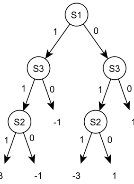
where u is the number of 1’s in the solution string, a portion of the population showed in Table 4.1 can be obtained by initializing those variables randomly. After initializing the population, the fitness value for each individual and the fitness difference value by

(20)

s1s2s3. . . s8 f df 111 01001 5 3 111 10100 5 3 111 01111 3 3 000 11111 7 1 000 00100 5 1 000 00001 5 1 000 10110 3 1 000 11100 3 1 001 01000 4 1 001 00011 3 1 001 00011 3 1 001 10100 3 1 010 01000 4 1 010 00100 4 1 010 01100 3 1 s1s2s3. . . s8 f df 010 10100 3 1 010 00111 2 1 010 11011 1 1 100 00000 5 -1 100 00100 4 -1 110 11111 5 -1 110 01101 1 -1 110 01111 0 -1 110 11011 0 -1 101 10000 3 -1 101 01101 1 -1 101 11110 0 -1 011 00001 3 -3 011 00110 2 -3 011 01111 0 -3

Table 4.1: Results obtained by perturbing variable s1.

grouped by the values of variables of sub-problem trap3(·), which the perturbed variable

s1 belongs to. From this table, it is clearly observed that the same solution to trap3(·) will

result in the same fitness difference value while other variables, i.e., s4, s5, . . . , s8, remain

no pattern to be recognized. Via the adopted decision learning algorithm, a decision tree as Figure 4.2 might be learned.

4.2 Algorithm Template

Based observations mentioned in section 4.1, the Inductive Linkage Identification (ILI) for non-overlapping sub-problems was proposed in [6, 30] and then modified in [33]. The pro-posed mechanism adopts the Inductive Dichotomiser 3 (ID3) [34] algorithm to construct the decision model, however, that concept does not restrict the choice of constructing algorithms. Therefore, this study integrates two distinct algorithms as the decision learn-ing components, denoted as ILI/ID3 and ILI/CART to indicate the different mechanisms they adopts. Since the adopted algorithms behave differently, insights from different as-pects might be obtained.

Algorithm 1 formulates the linkage detecting idea described in section 4.1: giving a problem definition f with ` variables and a population of size n, the perturbation and the decision tree construction are applied on variables sequentially. In the practical

(21)

imple-Figure 4.1: The decision tree learned from Table 4.1.

mentation, the populations are firstly split into subpopulations according to the values of the perturbed variable, then the decision learning are performed on those subpopulations. Once the tree is built, internal nodes are collected as a linkage set and indicating those variables are interdependent. After all variable are processed, all interactions should be identified as long as the given population size is sufficiently large.

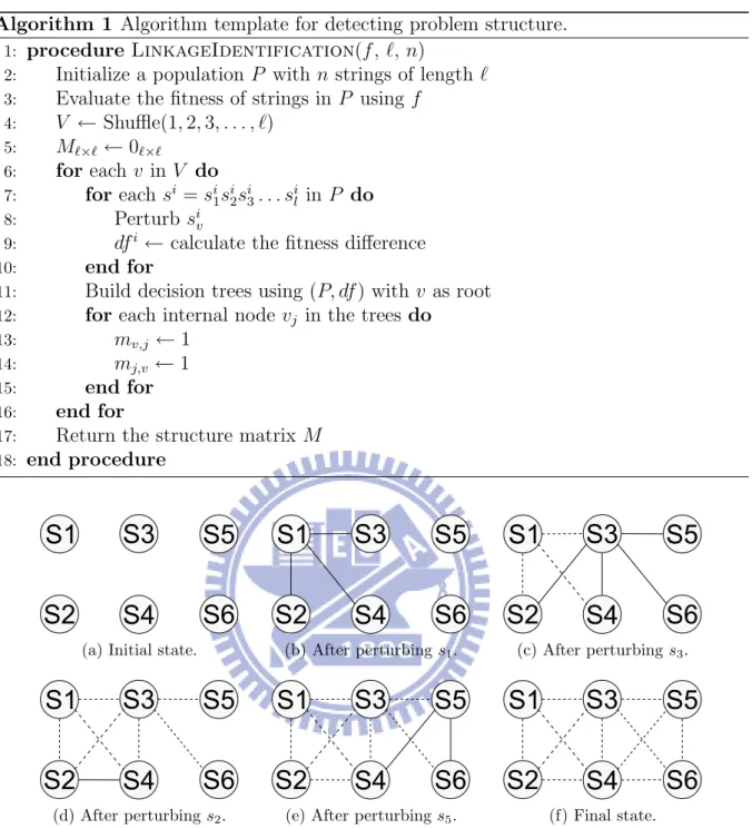
f (s1s2s3s4s5s6) = trap4(s1s2s3s4) + trap4(s3s4s5s6) (4.5)

Figure 4.2 illustrates an example problem defined as Equation 4.5. Initially, the

struc-ture matrix M6×6 is a zero-matrix indicating that there is no known interaction among

any variables as shown in Figure 4.2(a). After initialization, the modified ILI begins to

perturb variables in a randomly determined order: s1, s3, s2, s5, s4, and s6. By perturbing

and performing ID3 on variable s1, a linkage set {s1, s2, s3, s4} is recognized and indicates

that s1 interacts with s2, s3, and s4. Figure 4.2(b) shows the detected partial structure.

Notice that although s2, s3, and s4 belong to the same sub-problem as defined in

Equa-tion 4.5, there is no interacEqua-tion among them detected at the current iteraEqua-tion. Next,

when s3 is perturbed, ID3 identifies that s3 interacts with all other five variables since it

(22)

Algorithm 1 Algorithm template for detecting problem structure.

1: procedure LinkageIdentification(f , `, n)

2: Initialize a population P with n strings of length `

3: Evaluate the fitness of strings in P using f

4: V ← Shuffle(1, 2, 3, . . . , `) 5: M`×` ← 0`×`

6: for each v in V do

7: for each si = si₁si₂si₃. . . si_l in P do

8: Perturb si_v

9: dfi _{← calculate the fitness difference}

10: end for

11: Build decision trees using (P, df ) with v as root

12: for each internal node vj in the trees do

13: mv,j ← 1

14: mj,v ← 1

15: end for

16: end for

17: Return the structure matrix M

18: end procedure

(a) Initial state. (b) After perturbing s1. (c) After perturbing s3.

(d) After perturbing s2. (e) After perturbing s5. (f) Final state.

Figure 4.2: Problem structures detected during the linkage detection process. Dashed and solid lines represent known and newly discovered interactions respectively.

s2, s5, s4, and s6 sequentially. After all the variables are proceeded, the final structure is

constructed as shown in Figure 4.2(f).

Because there is no control parameter for the problem order/complexity, the obtained linkage information of the overall problem structure is unconstrained by any assumptions on the complexity of sub-problems. The only key factor in this condition regarding the correctness is whether or not the employed population is large enough for ILI to avoid

(23)

(a) Inductive Dichotomiser 3 (b) Classification and Regres-sion Tree

Figure 4.3: Decision tree constructed by different learning algorithms.

getting confused by the noise of fitness difference values. Our preliminary experiments involving different problem structures have shown that the proposed ILI modifications are able to construct correct problem structures as long as sufficiently large populations are utilized. For the purpose of gaining more understanding of the population size require-ment, we design and conduct more experiments to observe the scalability and flexibility, which are presented in chapter 5.

4.3 Adopted Decision Tree Learning Algorithms

This section briefly describe these two algorithms adopted in ILI. Figure 4.3 shows the learned model by different algorithms. As we can see, these two algorithm produce distinct decision trees from the same population due to their characteristics and behaviors. In order to obtain a better understanding of this idea of detecting linkages, the Inductive

Dichotomiser 3 [34] and Classification and Regression Tree [35] are respectively adopted

(24)

4.3.1 Inductive Dichotomiser 3 (ID3)

In the field of Machine Learning, the ID3 algorithm is probably the most mentioned and used mechanism as the example for lectures. This decision tree construction algorithm is a supervised categorization method working on discrete data sets, in which the datum entries consist of several decision variables and each decision variable is limited to certain predefined values. ID3 aims to build a decision tree according to entropy and information gain. Using a more mathematical description, let a category variable X have n possible

values {x1, x2, x3, . . . , xn}. The entropy of X is defined as:

Entropy(X) = −

n

X

i=1

p(xi) log(p(xi)) ,

where p(xi) is the probabilities for X being xi. The entropy can be regarded as the

indicator for how uniform the contents of a decision variable are. For example, a zero entropy value means that the variable always appears as a certain value, while a high entropy value indicates that there are many distinct values for the variable.

Let Y be a decision variable with m distinct values {y1, y2, y3, ...ym}. If X is somehow

affected by Y , it can be split into m subsets for m different values of Y , denoted as Xyi.

Based on the entropies, the interference of Y on X is written as the information gain:

Gain(X, Y ) = Entropy(X) − m X i=1 |Xyi| |X| Entropy(Xyi) .

Under this definition, higher values are obtained if the respective contents of each Xyi are

more identical, meaning that it is more suitable to classify X by Y .

When more decision variables are involved, says that X is affected by Y1, Y2, Y3, . . . ,

etc., the contributions of variables can be decided according to their information gains. By grouping the variables with the highest information gain, the training data set can be split into several subsets. Each subset contains the datum entries with a certain value of that variable. Then, the described procedure is applied on these subsets recursively until all the elements of each subset are identical, respectively. This procedure creates a

decision sequence which tells how different values of Yi result in different xi values of X.

The ID3 algorithm works in a greedy style, that is, after it choices the variable with the highest information gain and splits the population, that variable will not be investigated

(25)

again ever. This simple reduction performs efficiently when the decision model is not complex, e.g., variables are referred only once during the decision procedure. However, this assumption might be inappropriate for more complex problems, thus might causes complicated decision models.

4.3.2 Classification and Regression Tree (CART)

In the briefest description, the CART algorithm works similarly to the ID3 algorithm but differs in the following two ways. First, while the ID3 splits the population into subpopulations for each value of the splitting variable, the CART always splits it into two subpopulations and thus produces binary decision trees. When deciding how to split

the population, the CART will examine all possibilities of using every value yi of every

decision variable Y to split the population into two subpopulations, and the yi causing

the lowest impurity measure of the resultant two subpopulations will be selected as the splitting value and variable.

Second, the impurity measure for a given subpopulation t, i.e. a internal node, used in the CART is the Gini index defined as the following:

Gini(t) =X

i6=j

p(i|t) × p(j|t). (4.6)

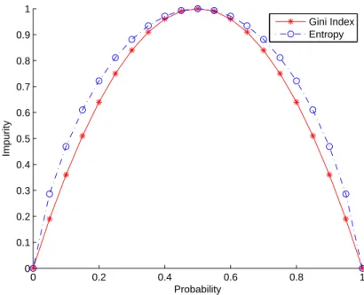
where i, j are the classifying categories and p(i|t), p(j|t) respectively refer to the pro-portions of i, j in the given node t. This definition can be interpreted as the expected probability of misclassification in the node t: by randomly selecting an object from the subpopulation and randomly assigning it to a category, the probability of that object is selected from i is p(i|t) and the probability of misclassification to j is p(j|t). There-fore, the higher value of Gini index measure refers to that misclassification occurs in the subpopulation more likely.

Figure 4.4 shows the distribution of both impurity measures, and there is little dif-ference can be seen from the plot. In fact, every impurity measure φ(p), where p is the probability of that a variable being a certain value, must satisfy the following require-ments:

(26)

0 0.2 0.4 0.6 0.8 1 0 0.1 0.2 0.3 0.4 0.5 0.6 0.7 0.8 0.9 1 Probability Impurity Gini Index Entropy

Figure 4.4: Comparison between the entropy and the Gini index.

Figure 4.5: The example of the third constraint of the impurity function. 2. φ(p) = φ(1 − p)

3. d

d2_pφ(p) < 0, 0 < p < 1

While the first and second constraints are intuitive conductions, the third one is required to ensure that the splitting producing purer subsets is preferred. For example, giving a set

R which can be somehow split, as Figure 4.5, into either {A1, A2} or {B1, B2} with the p denoted on the figure, the third constraint will lead to φ(0.2) + φ(0.2) > φ(0.4) + φ(0);

therefore the splitting R → {B1, B2} will be selected.

Since those impurity measuring functions distributes similarly under these constraints, the major behavioral difference should be caused by the splitting factors mentioned above. And how those differences contribute to the linkage identification task will be investigated in the chapter 5.

(27)

Chapter 5 Experiments

In this chapter, experiments designed to verify the capabilities of decision tree learning algorithms for linkage identification are presented. Firstly, the experimental methodology are described, and then issues from different aspect are investigated in sections. In depth discussions will addressed in the next chapter.

Since the adopted algorithms are both deterministic, both the time complexity and the space complexity can be expressed by the simpler measure on the population sizes. Thus our experiments are designed to find out the minimum required population sizes under every problem configurations.

For a given problem, firstly the population size assuring the successful trial of linkage identification, which means correctly identifying all the linkages within the problem for 29 times in 30 consecutive and independent runs, is obtained by doubling the population size from 2500 until the first successful trial is archived. Once the upper bound of

popu-lation size PU is found, the required population size is determined in a bisection manner:

The population size P = (PL + PU)/2 will be configured for the linkage identification

mechanism, where PL = 1 for the first iteration. If the mechanism can success with this

population size P , P will be regarded sufficiently large for the problem. The next

itera-tion will perform on the range [PL, P ]. Otherwise, the range [P, PU] will be used. This

procedure repeats until the range is small than a predefined distance, which is 2 in this study, and the last examined population size is considered as the minimal requirement for the problem.

(28)

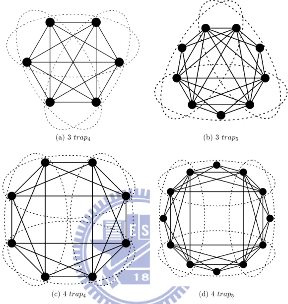
struc-(a) 3 trap4 (b) 3 trap5

(c) 4 trap4 (d) 4 trap5

Figure 5.1: Circular problem structures used in experiments.

tures hold certain good properties for experimental control. The number of linkages in-creases linearly with the number of sub-problems and so does the number of nodes. These easily controlled properties enable us to concentrate on the population requirement.

5.1 Requirements for Increasing Problem Sizes.

In the following experiments, circular structures with binary variables showed in Figure 5.1 are used to examine the scalability of increasing population sizes. For the experiments

of trap4 functions, each problem shares two variables with one of its neighbor

(29)

structure can be described as:

C4n(s1s2s3. . . s2n) =

n−1_X i=1

trap4(s2i−1s2is2i+1s2i+2) + trap4(s2n−1s2ns1s2) ,

(5.1)

where n is the number of sub-problems and greater than 2 to form a circle. For

exam-ple, C43(s1s2s3. . . s6) = trap4(s1s2s3s4) + trap4(s3s4s5s6) + trap4(s5s6s1s2) is the smallest

circular problem structure for trap4 under this definition as shown in Figure 5.1(a), and

inserting one more sub-problem will form a structure shown in Figure 5.1(c). The

overlap-ping scheme for trap5 functions is similar, except that each sub-problem has one unshared

variable. For example, the minimal circular structure of 3 trap5 functions, shown in

Fig-ure 5.1(b), can be put as

C53(s1s2s3. . . s9) = trap5(s1s2s3s4s5) + trap5(s4s5s6s7s8) + trap5(s7s8s9s1s2) ,

where s3, s6, and s9 are unshared.

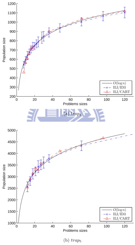
Figure 5.2 shows our experiment results on the two adopted algorithms. Regressions are made from results of ILI/ID3 to obtain the computational complexities, as well as the standard deviations are calculated.

5.2 Different Compositing Subproblems

Experiments examining the robustness on different functions are presented here. Three binary functions showed in Figure 5.3 are used as the subproblems for constructing the testing problems. The testing problems are all composed with order-4 subproblems in the same structure manner as experiments in section 5.1.

Results obtained by ILI/ID3 on these problems are compared with the trap4 function

being the baseline. Since the similarity between ILI/ID3 and ILI/CART under the same sub-function size has been verified in section 5.1, there should be an analog to ILI/CART for these empirical results on the robustness. Therefore those problems are not experi-mented with ILI/CART specifically.

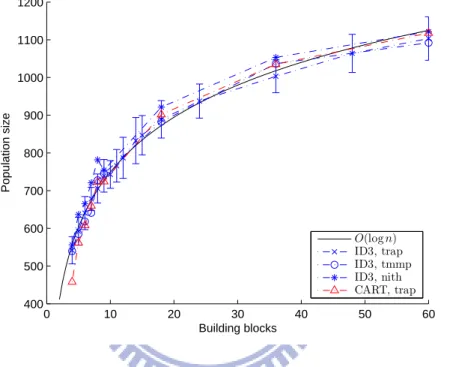
Figure 5.4 shows the experiment results of both ILI/ID3 and ILI/CART. The standard

(30)

0 20 40 60 80 100 120 200 300 400 500 600 700 800 900 1000 1100 1200 Problems sizes Population size O(log n) ILI/ID3 ILI/CART (a) trap4 0 20 40 60 80 100 120 1000 1500 2000 2500 3000 3500 4000 4500 5000 Problems sizes Population size O_{(log n)} ILI/ID3 ILI/CART (b) trap5

(31)

0 1 2 3 4 0 1 2 3 4 Unitation Function Value trap4

(a) trap4function

0 1 2 3 4 0 1 2 3 4 Unitation Function Value nith4 (b) nith4function 0 1 2 3 4 0 1 2 3 4 Unitation Function Value tmmp4 (c) tmmp4 function

Figure 5.3: Functions used as the subproblems in section 5.2.

0 10 20 30 40 50 60 400 500 600 700 800 900 1000 1100 1200 Building blocks Population size O_{(log n)} ID3, trap ID3, tmmp ID3, nith CART, trap

Figure 5.4: Required population sizes for different composing subproblems.

regression based on trap4 using the ID3 algorithm as the decision tree learning mechanism

is plotted.

5.3 Insensitivity to Substructures

The series of experiments in this section aims to examine the capability of detecting problem structures composed of sub-structures. Separate circular problem structures form a large problem structure, and the population requirement of the modified ILI is compared to that for larger structures of the same problem size. In these experiments, circular problem structures composed of m smaller sub-structures are defined as

C4m n =

m−1_X i=0

(32)

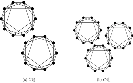
(a) C42

n (b) C43n

Figure 5.5: Circular problem structures composed of separate sub-structures, where n = 5. In this definition, those sub-problems of a sub-structure are depended in the circular manner, while there exist no dependencies among sub-structures.

Figure 5.5 shows examples of circular structures composed of two and three

sub-structures of five trap4 sub-problems. Experimental results on those problem structures,

C42

n, and C43n, are shown in Figure 5.6. Those results are compared with the

prob-lem structure involving no sub-structure, C4n, to find out whether additional efforts are

required to detect inner structures.

5.4 High Cardinality Variables

The experiments described so far are performed on binary variables, thus observations can be focused on the influences of the problem structures on requirements of population sizes. In this section, we try to investigate the scalability of variables by extending variables to higher cardinalities, whose variables have more discrete values to be assigned.

Two major differences of experiment configurations are made while the problem struc-tures remain unchanged as section 5.1: first, the function defined as Equation 5.2 is

(33)

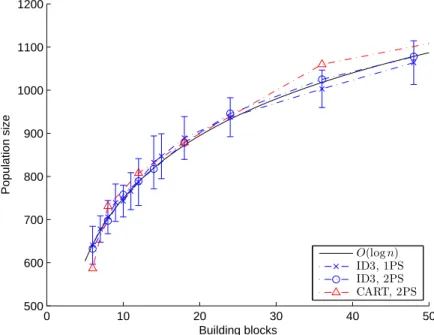
0 10 20 30 40 50 500 600 700 800 900 1000 1100 1200 Building blocks Population size O_{(log n)} ID3, 1PS ID3, 2PS CART, 2PS

Figure 5.6: Circular problem structures composed of one, two, and three sub-structures

with trap4 as the elementary sub-problems.

adopted as the subproblem in response to the extension of high-cardinality.

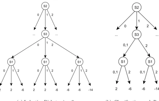
f unch(x1x2x3s4) =        8h, if xi = h for all xi; 4h − x1− x2− x3− x4, otherwise. , (5.2)

where h is the cardinality of those variables, e.g., h = 3 refers to xi ∈ {0, 1, 2}. This

function proposed in [36] is designed for researching the extended version of ECGA for integers, integer extended compact genetic algorithm (iECGA). This function holds the deceptive property and thus is called a “deceptive function.” In deceptive functions, since the trends of fitness distributions and the global optimum locate oppositely on the landscape, traditional hill-climbing techniques would fail for these problems. Therefore, those functions are widely used in evolutionary algorithms as testing problems.

Another modification is made on the perturbation operator. For binary variables, the perturbation is defined as flipping between 0 and 1. When considering the generality, this binary operation can be regarded as a function involving an addition with a modulus followed, which is denoted by Equation 5.3:

(34)

2 3 4 5 6 7 0 10 20 30 40 50 60 70 80 90 100 Cardinality Success rate (%) BBs = 3, CART BBs = 5, CART BBs = 10, CART BBs = 3, ID3 BBs = 5, ID3 BBs = 10, ID3

Figure 5.7: Success rates against cardinalities of variables.

where the operator ⊕ refers to the modulus operation and the subindex 2 indicates the binary cardinality. Following this definition, a perturbation operator of h-cardinality variables can be generalized as:

perturbh(x) = (x + 1) ⊕ h (5.4)

From our preliminary experiments, we found that obtaining the required population sizes becomes a time-consuming task especially when the cardinality get higher. There-fore, experiments in this section are designed to find the probabilities of successful linkage identifications with increasing cardinalities under a given population size. The experiment results are drawn from 40 independent runs under population size 30000 with different configurations, and showed in Figure 5.7.

(35)

Chapter 6 Discussion

6.1 Logarithmic Scalability

From the experiments described in 5.1 and the Figure 5.2, two observations on the scala-bility of problem sizes can be made. The first one is that the results can be well fitted by using logarithmic curves. Such a phenomenon implies that the required population size grows logarithmically with respect to the number of sub-problems and indicates the pro-posed approach is quite efficient and scalable on the circular problem structures adopted in the experiments. The population size growth rate is also similar to that required by the original ILI on non-overlapping building blocks as reported in the literature [30]. Sec-ondly, since the growth of the required population size can be well fitted with logarithmic

curves for both trap4 and trap5 functions, this approach should require similar population

sizes for the problems of similar structures.

In our experiment for sub-structures, whose results are shown in Figure 5.6, the

re-quired population sizes of C42

n and C43n are very close to that of C4n when the overall

problem sizes are identical. All the experimental results are therefore well fitted by the

same logarithmic curve that fits the results of C4n. Such an outcome indicates that the

modified ILI is able to correctly identify isolated as well as interdependent parts of a large problem structure without extra cost.

Another observation is that the experiment results obtained by ILI/ID3 and ILI/CART are almost identical. These results indicate the same computational complexity held by the two decision tree learning algorithms when the problem structures are the same and composed of binary variables.

(36)

6.2 Robustness against Composing Subproblems

Using different functions as the composing subproblems, the results of experiments on the robustness are showed in Figure 5.4. These experiment results verifies the idea implied by Equation 4.2: linkage identification by decision learning should work as long as the perturbation operates deterministically, i.e., the perturbation on the same context of variables of the sub-functions will results in the same fitness difference value.

It can be obviously observed that this linkage identification methods require the same problem size when the problem structures and the variable domains are both the same, despite the functions used as subproblems. This observation indicates the robustness when different subproblem involved in the overall problem.

6.3 Scalability of the Variable Cardinality

From the experiments described in section 5.4, the results on the scalability of the variable cardinality are showed. Although the success probabilities of both ILI/ID3 and ILI/CART decrease when the cardinality gets higher, ILI/CART decreases more slower while ILI/ID3 falls quickly. This phenomena indicates that ILI/CART holds the better scalability on variables and thus might are more suitable when applied on unknown problems.

The difference between these two implementation might result from the different mech-anisms of subpopulation-splitting. While ID3 algorithm produces subpopulations for each value of the selected variable, produced subpopulations thus contain fewer instances. As a consequence, those instances in a subpopulation might not be able to provide sufficient information for correct decision tree constructions in the following iterations. Therefore, compared with ILI/CART, the lower chances for successful linkage identifications are obtained with ILI/ID3 when the same population size are provided. However, this pre-sumption needs to be further studied and experimented, so that the influences of different splitting scenarios can be discovered.

(37)

Chapter 7 Conclusions

In this thesis, we extended the inductive linkage identification to detect general problem structures composed of overlapping sub-problems and conducted experiments by using circular overlapping structures for gaining more insights and understandings. According to the experimental observations, the proposed technique was found able to correctly detect circular problem structures and require a population size growing logarithmically with the problem size. The population requirement was observed insensitive to the problem structure consisting of similar sub-structures for the identical overall problem size.

In addition to the influence of problem structures, experiments for investigating the problem complexity caused by variables are also performed. While ILI/ID3 and ILI/CART both perform efficiently on binary variables, high cardinality variables cause different difficulties to these two approaches. Our results show that the success probability of ILI/CART decreases much more slower than ILI/ID3 under the same population size, this observation indicates the better scalability are held when the CART algorithm is adopted for the linkage identification.

One of the major differences between ILI and most of the other existing linkage learning methods is the absence of algorithmic parameters for the complexity of sub-problems. The proposed modifications of ILI keep this feature unchanged. Since ILI performs the task of linkage identification without assumptions on the problem structure, such as the chosen probabilistic model or the maximum degree of interactions, the relationship among variables should be extracted as authentic as possible.

(38)

be applied in two ways. Firstly, by serving as a preprocessor of genetic algorithms, the proposed technique can express the dependencies among variable as a graph such that delicately-designed genetic, linkage-aware operators, such as CrossNet [5], or certain processing mechanisms may utilize the linkage information to preserve and exchange the building blocks. Secondly, the proposed technique can be employed to inspect and extract the relationship among decision variables for understanding the inner structure of the problem at hand in order to assist potential further applicable operations or be integrated in some advanced frameworks, such as the concept of data-centric grey-box optimization in Optinformatics [37, 38].

(39)

Bibliography

[1] J. H. Holland, Adaptation in natural and artificial systems. Cambridge, MA, USA: MIT Press, 1992.

[2] D. E. Goldberg, Genetic Algorithms in Search, Optimization and Machine Learning. Boston, MA, USA: Addison-Wesley Longman Publishing Co., Inc., 1989. [Online]. Available: http://portal.acm.org/citation.cfm?id=534133

[3] D. E. Goldberg, The Design of Innovation: Lessons from and for Competent Genetic

Algorithms. Norwell, MA, USA: Kluwer Academic Publishers, 2002.

[4] D. E. Goldberg, B. Korb, and K. Deb, “Messy genetic algorithms: Motivation, anal-ysis, and first results,” Complex Systems, vol. 3, no. 5, pp. 493–530, 1989.

[5] F. Stonedahl, W. Rand, and U. Wilensky, “Crossnet: a framework for crossover with network-based chromosomal representations,” in Proceedings of ACM SIGEVO

Genetic and Evolutionary Computation Conference 2008 (GECCO-2008), 2008, pp.

1057–1064.

[6] C.-Y. Chuang and Y.-p. Chen, “Linkage identification by perturbation and decision tree induction,” in Proceedings of 2007 IEEE Congress on Evolutionary Computation

(CEC 2007), 2007, pp. 357–363.

[7] M. Munetomo and D. E. Goldberg, “Identifying linkage groups by nonlinearity/non-monotonicity detection,” in Proceedings of Genetic and Evolutionary Computation

Conference 1999 (GECCO-99), vol. 1, 1999, pp. 433–440.

[8] H. Kargupta, “SEARCH, polynomial complexity, and the fast messy genetic algo-rithm,” Ph.D. dissertation, University of Illinois, 1995.

(40)

[9] G. Harik, “Learning gene linkage to efficiently solve problems of bounded difficulty using genetic algorithms,” Ph.D. dissertation, University of Illinois, 1997.

[10] H. M¨uhlenbein and G. Paaß, “From recombination of genes to the estimation of dis-tributions i. binary parameters,” in Proceedings of the 4th International Conference

on Parallel Problem Solving from Nature (PPSN IV), 1996, pp. 178–187.

[11] P. Larra˜naga and J. A. Lozano, Estimation of Distribution Algorithms: A New Tool

for Evolutionary Computation, ser. Genetic algorithms and evolutionary

computa-tion. Boston, MA: Kluwer Academic Publishers, October 2001, vol. 2.

[12] M. Pelikan, D. E. Goldberg, and F. G. Lobo, “A survey of optimization by build-ing and usbuild-ing probabilistic models,” Computational Optimization and Applications, vol. 21, no. 1, pp. 5–20, 2002.

[13] S. Baluja, “Population-based incremental learning: A method for integrating genetic search based function optimization and competitive learning,” Pittsburgh, PA, USA, Tech. Rep., 1994.

[14] G. R. Harik, F. G. Lobo, and D. E. Goldberg, “The compact genetic algorithm,”

IEEE Transactions on Evolutionary Computation, vol. 3, no. 4, pp. 287–297,

Novem-ber 1999.

[15] J. de Bonet, C. Isbell, and P. Viola, “MIMIC: Finding optima by estimating proba-bility densities,” in Advances in Neural Information Processing Systems, vol. 9, 1997, pp. 424–430.

[16] S. Baluja and S. Davies, “Using optimal dependency-trees for combinational opti-mization,” in Proceedings of the Fourteenth International Conference on Machine

Learning (ICML ’97), 1997, pp. 30–38.

[17] M. Pelikan and H. M¨uhlenbein, “The bivariate marginal distribution algorithm,” in Advances in Soft Computing - Engineering Design and Manufacturing, 1999, pp. 521–535.

(41)

[18] G. Harik, “Linkage learning via probabilistic modeling in the ECGA,” Illinois Genetic Algorithms Laboratory, University of Illinois at Urbana-Champaign, IlliGAL Report No. 99010, 1999.

[19] M. Pelikan, D. E. Goldberg, and E. Cant´u-Paz, “BOA: The Bayesian optimization algorithm,” in Proceedings of Genetic and Evolutionary Computation Conference

1999 (GECCO-99), vol. 1, 1999, pp. 525–532.

[20] H. M¨uhlenbein and T. Mahnig, “FDA - A scalable evolutionary algorithm for the optimization of additively decomposed functions,” Evolutionary Computation, vol. 7, no. 4, pp. 353–376, 1999.

[21] H. M¨uhlenbein and R. H¨ons, “The estimation of distributions and the minimum relative entropy principle,” Evolutionary Computation, vol. 13, no. 1, pp. 1–27, 2005. [22] L. R. Emmendorfer and A. T. R. Pozo, “Effective linkage learning using low-order

statistics and clustering,” 2009.

[23] H. Kargupta, “The gene expression messy genetic algorithm,” in Proceedings of IEEE

International Conference on Evolutionary Computation, 1996, 1996, pp. 814–819.

[24] M. Munetomo and D. Goldberg, “Identifying linkage by nonlinearity check,” Illinois Genetic Algorithms Laboratory, University of Illinois at Urbana-Champaign, IlliGAL Report No. 98012, 1998.

[25] R. B. Heckendorn and A. H. Wright, “Efficient linkage discovery by limited probing,”

Evolutionary Computation, vol. 12, no. 4, pp. 517–545, 2004.

[26] S. Zhou, Z. Sun, and R. B. Heckendorn, “Extended probe method for linkage discov-ery over high-cardinality alphabets,” in Proceedings of ACM SIGEVO Genetic and

Evolutionary Computation Conference 2007 (GECCO-2007), 2007, pp. 1484–1491.

[27] S. Zhou, R. B. Heckendorn, and Z. Sun, “Detecting the epistatic structure of gener-alized embedded landscape,” Genetic Programming and Evolvable Machines, vol. 9, no. 2, pp. 125–155, June 2008.

(42)

[28] M. Tsuji, M. Munetomo, and K. Akama, “Linkage identification by fitness difference clustering,” Evolutionary Computation, vol. 14, no. 4, pp. 383–409, 2006.

[29] E. D. de Jong, R. Watson, and D. Thierens, “On the complexity of hierarchical prob-lem solving,” in Proceedings of Genetic and Evolutionary Computation Conference

2005 (GECCO-2005), 2005, pp. 1201–1208.

[30] C.-Y. Chuang and Y.-p. Chen, “Recognizing problem decomposition with inductive linkage identification: Population requirement vs. subproblem complexity,” in

Pro-ceedings of the Joint 4th International Conference on Soft Computing and Intelligent Systems and 9th International Symposium on advanced Intelligent Systems (SCIS & ISIS 2008), 2008, pp. 670–675.

[31] D. H. Ackley, A connectionist machine for genetic hillclimbing. Kluwer Academic

Publishers, 1987.

[32] K. Deb and D. E. Goldberg, “Analyzing deception in trap functions,” in Proceedings

of the Second Workshop on Foundations of Genetic Algorithms (FOGA 92), 1992,

pp. 93–108.

[33] Y.-W. Huang and Y.-p. Chen, “On the detection of general problem structures by using inductive linkage identification,” in Proceedings of ACM SIGEVO Genetic and

Evolutionary Computation Conference 2009 (GECCO-2009), 2009, pp. 1853–1854.

[34] J. R. Quinlan, “Induction of decision trees,” in Readings in knowledge acquisition

and learning: automating the construction and improvement of expert systems. San

Francisco, CA, USA: Morgan Kaufmann Publishers Inc., 1993, pp. 349–361.

[35] L. Breiman, J. Friedman, C. J. Stone, and R. A. Olshen, Classification and Regression

Trees, 1st ed. Chapman & Hall/CRC, January 1984.

[36] P. C. Hung and Y. P. Chen, “iecga: integer extended compact genetic algorithm,” in

GECCO ’06: Proceedings of the 8th annual conference on Genetic and evolutionary computation. New York, NY, USA: ACM, 2006, pp. 1415–1416.

(43)

[37] M. N. Le and Y. S. Ong, “A frequent pattern mining algorithm for understanding genetic algorithms,” in Proceedings of International Conference on Intelligent

Com-puting 2008 (ICIC 2008), 2008.

[38] M. N. Le, Y. S. Ong, and Q. H. Nguyen, “Optinformatics for schema analysis of binary genetic algorithms,” in Proceedings of Genetic and Evolutionary Computation

基於決策樹學習的變數相依性測定法

國

立

交

通

大

學

資訊科學與工程研究所

碩

碩

碩

碩

士

士

士

士

論

論

論

論

文

文

文

文

基 於 決 策 樹 學 習 的 變 數 相 依 性 測 定 法

Linkage Identification Based on Decision Tree Learning

研 究 生：黃淵暐

指導教授：陳穎平 教授

中

中

中

中

華

華

華

華

民

民

民

民

國

國

國

國

九

九

九

九

十

十

十

十

九

九

九

九

年

年

年

年

六

六

六

六

月

月

月

月

基於決策樹學習的變數相依性測定法

Linkage Identification Based on Decision Tree Learning

研 究 生：黃淵暐 Student：Yuan-wei Huang

指導教授：陳穎平 Advisor：Ying-ping Chen

國 立 交 通 大 學

資 訊 科 學 與 工 程 研 究 所

碩 士 論 文

基於決策數學習的變數相依性測定法

Linkage Identification Based on Decision Tree Learning

學生：黃淵暐

指導教授：陳穎平 教授

國立交通大學 資訊科學與工程研究所

基於決策樹學習的變數相依性測定法

研究生：黃淵暐

指導教授：陳穎平教授

研究生：黃淵暐 Student：Yuan-wei Huang

國立交通大學

資訊科學與工程研究所

碩士論文

指導教授：陳穎平教授

國立交通大學資訊科學與工程研究所